The effect of harmonized emissions on aerosol properties in global models – an AeroCom experiment

(1)

ACPD

7, 1699–1723, 2007

AeroCom: e_ffect of harmonized emissions in aerosol

modeling

C. Textor et al.

Title Page

Abstract Introduction

Conclusions References

Tables Figures

◭ ◮

Back Close

Full Screen / Esc

Printer-friendly Version

Interactive Discussion

Atmos. Chem. Phys. Discuss., 7, 1699–1723, 2007 www.atmos-chem-phys-discuss.net/7/1699/2007/ © Author(s) 2007. This work is licensed

under a Creative Commons License.

Atmospheric Chemistry and Physics Discussions

The e

_ff

ect of harmonized emissions on

aerosol properties in global models – an

AeroCom experiment

C. Textor1,19, M. Schulz1, S. Guibert1, S. Kinne2, Y. Balkanski1, S. Bauer3, T. Berntsen4, T. Berglen4, O. Boucher5,18, M. Chin16, F. Dentener6, T. Diehl17, J. Feichter2, D. Fillmore7,1, P. Ginoux9, S. Gong10, A. Grini4, J. Hendricks11, L. Horowitz9, P. Huang10, I. S. A. Isaksen4, T. Iversen4, S. Kloster2,6, D. Koch3, A. Kirkev ˚ag4, J. E. Kristjansson4, M. Krol6,12, A. Lauer11, J. F. Lamarque7, X. Liu13,8, V. Montanaro14, G. Myhre4, J. E. Penner13, G. Pitari14, S. Reddy5,9, Ø. Seland4, P. Stier2,20, T. Takemura15, and X. Tie7

1

Laboratoire des Sciences du Climat et de l’Environnement, Gif-sur-Yvette, France

2

Max-Planck-Institut f ¨ur Meteorologie, Hamburg, Germany

3

Columbia University, GISS, New York, USA

4

University of Oslo, Department of Geosciences, Oslo, Norway

5

Laboratoire d’Optique Atmosph ´erique, Universit ´e des Sciences et Technologies de Lille, CNRS, Villeneuve d’Ascq, France

6

European Commision, Joint Research Centre, Institute for Environment and Sustainability, Climate Change Unit, Italy

7

NCAR, Boulder, Colorado, USA

8

Battelle, Pacific Northwest National Laboratory, Richland, USA

(2)

ACPD

7, 1699–1723, 2007

modeling

C. Textor et al.

Title Page

Tables Figures

◭ ◮

Back Close

Full Screen / Esc

Interactive Discussion 9

NOAA, Geophysical Fluid Dynamics Laboratory, Princeton, New Jersey, USA

10

ARQM Meteorological Service Canda, Toronto, Canada

11

DLR-Institut f ¨ur Physik der Atmosph ¨are, Oberpfaffenhofen, Germany

12

Institute for Marine and Atmospheric Research Utrecht (IMAU) Utrecht University, The Netherlands

13

University of Michigan, Ann Arbor, MI, USA

14

Universita degli Studi L’Aquila, Italy

15

Kyushu University, Fukuoka, Japan

16

NASA Goddard Space Flight Center, Greenbelt, MD, USA

17

Goddard Earth Sciences and Technology Center, University of Marylan Baltimore County, Baltimore, Maryland, USA

18

Hadley Centre, Met Office, Exeter, United Kingdom

19

Service d’A ´eronomie, CNRS/UPMC/IPSL, Paris, France

20

Department of Environmental Science and Engineering, California Institute of Technology, Pasadena, USA

Received: 18 December 2006 – Accepted: 19 January – Published: 2 February 2007 Correspondence to: C. Textor (christiane.textor@aero.jussieu.fr)

(3)

ACPD

7, 1699–1723, 2007

modeling

C. Textor et al.

Title Page

Tables Figures

◭ ◮

Back Close

Full Screen / Esc

Interactive Discussion Abstract

The e_ffects of unified aerosol sources on global aerosol fields simulated by di_fferent

models are examined in this paper. We compare results from two AeroCom

experi-ments, one with different (ExpA) and one with unified emissions, injection heights, and

particle sizes at the source (ExpB). Surprisingly, harmonization of aerosol sources has

5

only a small impact on the simulated diversity for aerosol burden, and consequently optical properties, as the results are largely controlled by model-specific transport, removal, chemistry (leading to the formation of secondary aerosols) and parameter-izations of aerosol microphysics (e.g. the split between deposition pathways) and to a lesser extent on the spatial and temporal distributions of the (precursor) emissions.

10

The burdens of black carbon and especially sea salt become more coherent in ExpB only, because the large ExpA diversity for these two species was caused by few out-liers. The experiment also indicated that despite prescribing emission fluxes and size distributions, ambiguities in the implementation in individual models can lead to

sub-stantial di_fferences.

15

These results indicate the need for a better understanding of aerosol life cycles at process level (including spatial dispersal and interaction with meteorological parame-ters) in order to obtain more reliable results from global aerosol simulations. This is particularly important as such model results are used to assess the consequences of specific air pollution abatement strategies.

20

1 Introduction

One of the largest uncertainties in assessing the human impact on climate is related to the role of aerosol and clouds (IPCC, 2001). The Aerosol inter Comparison project

Ae-roCom (http://nansen.ipsl.jussieu.fr/AEROCOM) attempts to advance the

understand-ing of the global aerosol and its impact on climate by performunderstand-ing a systematic analysis

25

of the results of more than 16 global aerosol models including a comparison with a

(4)

ACPD

7, 1699–1723, 2007

modeling

C. Textor et al.

Title Page

Tables Figures

◭ ◮

Back Close

Full Screen / Esc

large number of satellite and surface observations (Guibert et al., 20071; Kinne et al.,

2006; Schulz et al., 2006; Textor et al., 2006). In these studies, it was found that signif-icant uncertainty in global modeling of spatial aerosol mass distributions is associated with aerosol processes.

The aerosol mass distributions depend on spatial and temporal distribution of

emis-5

sions (of aerosols and precursors), on the ambient conditions (e.g., humidity or pre-cipitation) and the transport in the atmosphere as described by the global transport models, as well as on the aerosol microphysical processes (e.g., water uptake or deposition, and chemistry for secondary aerosols) as described by the implemented aerosol module. All these model components are inter-related, since aerosol mass is

10

conserved. AeroCom focuses on five most important aerosol components: dust (DU), sea salt (SS), sulfate (SO4), black carbon (BC), and particulate organic matter (POM), and the sum of these components (AER).

In a first set of simulations (AeroCom ExpA, see Textor et al. (2006)) each model was run with emission data for each aerosol component chosen by the individual

par-15

ticipating groups. In these simulations, emission data di_ffered not only because of the

use of diverse data sources, but even when referring to the same data source due to

different implementation into the models (e.g. regridding, size-assumptions). In order

to remove the impact of emission diversity on aerosol simulations a sensitivity exper-iment was performed (AeroCom ExpB) where unified global emission data sets for

20

primary aerosol and aerosol precursors for the year 2000 (Dentener et al., 2006) were prescribed.

1

Guibert, S., Schulz, M., Kinne, S., Textor, C., Balkanski, Y., Bauer, S., Berntsen, T., Berglen, T., Boucher, O., Chin, M., Dentener, F., Diehl, T., Feichter, H., Fillmore, D., Ghan, S., Ginoux, P., Gong, S., Grini, A., Hendricks, J., Horowitz, L., Isaksen, I., Iversen, T., Kloster, S., Koch, D., Kirkevag, A., Kristjansson, J. E., Krol, M., Lauer, A., Lamarque, J. F., Liu, X., Montanaro, V., Myhre, G., Penner, J., Pitari, G., Reddy, S., Seland, Ø., Stier, P., Takemura, T., and Tie, X.: Comparison of lidar data with model results from the aerocom intercomparison project, in preparation, 2007.

(5)

ACPD

7, 1699–1723, 2007

modeling

C. Textor et al.

Title Page

Tables Figures

◭ ◮

Back Close

Full Screen / Esc

In this study we compare simulated global mass distributions and underlying pro-cesses in AeroCom ExpA and ExpB. In the next two sections we summarize the model-setups and emissions. Then, changes in the diversity of simulated global total aerosol mass distributions are presented and discussed in the context of spatial distributions

and residence times of the different aerosol components. New radiative forcing

esti-5

mates obtained from ExpB and an additional experiment with unified sources for pre-industrial conditions are discussed in Schulz et al. (2006). Supplementary maps and vertical profiles, and many other quantities are provided on the AeroCom web site (http://nansen.ipsl.jussieu.fr/AEROCOM/data.html).

2 Model setup 10

A comprehensive description of the AeroCom models including a table linking model name abbreviations to the model versions actually used can be found in Textor et al. (2006). The model configurations did not change between ExpA and ExpB, ex-cept for three models: in the DLR model, coarse aerosols have been implemented only in ExpB. Larger changes have been made in KYU, where the interaction between

15

aerosols and clouds has been included for ExpB, and carbonaceous aerosols (BC and POM) are treated externally, unlike the internal treatment in ExpA. In LOA, dry turbulent deposition is only considered in ExpA. In addition, deviations from the recommended AeroCom emissions occurred: In KYU and UIO GCM, sources of DU and SS remained those of ExpA. In KYU B, only the emitted aerosol mass flux was matched, but size

dis-20

tributions have not been adapted. In ARQM, emissions have been modified for ExpB, but did not follow the ExpB recommendations. In MATCH, SS sources remained those of ExpA. Due to these deviations, all results of DLR, KYU, LOA, and ARQM, SS results of MATCH and UIO-GCM, and DU results of UIO GCM are discussed, but not included

in the calculation of the model diversities shown in Fig.1 and Tables1–6. Due to this

25

sampling procedure, the statistics on ExpA reported in this paper does not entirely match the results reported in Textor et al. (2006).

(6)

ACPD

7, 1699–1723, 2007

modeling

C. Textor et al.

Title Page

Tables Figures

◭ ◮

Back Close

Full Screen / Esc

The ExpA emissions are discussed in detail by Textor et al. (2006). Models agree less on the sources of the “natural” aerosol components, SS and DU. This is caused

by di_fferences in the simulated size spectrum of the emitted particles, by di_fferences in

the parameterizations of source strength as a function of wind speed (and soil

prop-erties for DU), and by di_fferences in the wind fields themselves. Emissions of the

5

“anthropogenic” species (SO4, BC, and POM) show better agreement, because of the common use of some few, and usually similar emission inventories. However, these inventories have often been improved for certain species or emission types by the indi-vidual modelers, and their mix in each of the ExpA models is variable, see references in Textor et al. (2006).

10

The unified emission data used in ExpB have been recompiled from various recently published inventories, augmented with data generated for the purpose of the AeroCom ExpB as explained in detail by Dentener et al. (2006). The inventory includes fluxes for “natural” emissions of mineral DU, SS, dimethyl sulfide (DMS) from the oceans,

sulfur dioxide (SO₂) from volcanoes, sulfate and carbon from natural wild-land fires,

15

and particulate organic carbon including secondary organic aerosol. In addition,

an-thropogenic emissions from biomass burning and fossil fuel burning of SO₂, particulate

organic matter and black carbon are provided. The prescribed emission fields are

gen-erated on a global 1◦

×1◦spatial resolution, and a temporal resolution ranging from daily

to annual. Injection heights for volcanic and wildfire emissions, and size distributions of

20

the primary particulate emissions are prescribed. In this paper we focus on the

emis-sions representative for present-day conditions. The models were nudged to (different)

meteorological data sets for the year 2000. Four models, which could only operate in a climatological mode (ULAQ, UIO GCM, ARQM, and DLR), provided averages from 5 years of simulation.

25

(7)

ACPD

7, 1699–1723, 2007

modeling

C. Textor et al.

Title Page

Tables Figures

◭ ◮

Back Close

Full Screen / Esc

Interactive Discussion 3 Results

3.1 Emissions

A comparison of the emissions in ExpA and ExpB shows that in most models the mass fluxes of “natural” aerosols (coarser sized SS and DU) are larger (on average by 77% and by 9%, respectively). The emissions of carbonaceous emissions, BC and POM,

5

are on average by 33% and by 23%, respectively, smaller. The total SO4 sources decreased by 8%, see below for a discussion. For the model-average relative changes

of the source mass fluxes see also Table7.

The implementation of the unified AeroCom sources in ExpB strongly reduced the diversity of global annual emission mass fluxes when compared to ExpA. However,

10

some differences in the emissions remained due to model-specific representations of

the particle size distributions (bin schemes or modal schemes, and the number of modes or bins), or simply by inaccurate implementation. In addition, the initial degree of the mixing height is governed by the model architecture (e.g., height of model levels and the emission scheme). Some further discrepancies were caused by the use of

15

intermediate versions of the AeroCom emission data.

The model diversity, i.e., the scatter of the model results, is defined here as the standard deviation of the globally and annually averaged model results, normalized by the all-models-average, for a detailed discussion see Textor et al. (2006). Model diversities along with all-model-averages and all-model medians for the annually and

20

globally averaged source fluxes are given in Tables1–6. The large emission

mass-flux diversities in ExpA are sharply reduced in ExpB to less than 5%, except for SO4. The diversity of the total SO4 source in ExpB (21%) is almost as large as in ExpA (25%). SO4 originates predominantly (about 97% on average in both experiments) from model-specific chemical production as sulfur-containing precursor gases (DMS

25

and SO₂) are oxidized. Direct emission of SO4 decreased by 11% and that of the

precursor gases SO2 and DMS by 11% and 50%, respectively, in ExpB. 79% (90%)

of the secondary SO4 stems from SO₂, and 21% (10%) from DMS oxidation in ExpA

(8)

ACPD

7, 1699–1723, 2007

modeling

C. Textor et al.

Title Page

Tables Figures

◭ ◮

Back Close

Full Screen / Esc

(ExpB). A comparison of the individual processes involved in the sulphur cycle shows,

that the diversity in SO4 sources is due to di_fferences in precursor gas emissions,

but di_fferences in the dry deposition of these gases and the chemical production are

as important. This leads to the larger diversity of SO4 when compared to the other aerosol components. Note however, that the statistics of the sulfur cycle is based on

5

only four models, which delivered all quantities involved for both experiments.

3.2 Total mass

The changes in (global annual) masses for individual aerosol components between ExpA and B are generally consistent with those for emissions: models with increased emissions show larger mass and vice versa. However, this is not true, when diversity

10

in size assumptions comes into play, as for DU and SS. For the model-average relative

changes of the total masses see also Table7.

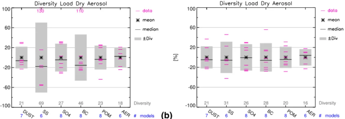
The associated model diversities of the simulated global annual masses are shown

in Fig.1, and in Tables1–6. Surprisingly, mass diversity is not considerably smaller

in ExpB with harmonized emission mass-fluxes. The apparent strong decrease in

15

mass diversities for SS and BC in ExpB results from a few strong outliers in ExpA that are removed in ExpB. These results indicate that diversities for the simulated aerosol

mass depend largely on di_fferences of model-specific transports and parameterizations

aerosol interactions with its environment and microphysical processes, and to a lesser extend on their (precursor) emissions.

20

3.3 Spatial distributions

Horizontal and vertical dispersal di_ffers considerably among models that participated in

AeroCom experiments (Textor et al., 2006). Meridional dispersal (represented here as mass fractions in polar regions) and vertical dispersal (as mass fractions above 5 km

altitude) simulated in ExpA and ExpB are compared in Fig.2. Model diversities for

po-25

lar and upper troposphere mass fractions (Tables1–6) are similar in two experiments,

(9)

ACPD

7, 1699–1723, 2007

modeling

C. Textor et al.

Title Page

Tables Figures

◭ ◮

Back Close

Full Screen / Esc

and the more detailed analysis in Fig.2shows, that the aerosol dispersal did not

signif-icantly change between the two experiments. Spatial dispersal is more similar for any pair of simulations performed by an individual model than among all models using the same emissions in ExpB. Thus, meridional and vertical dispersals seem to be

deter-mined by the model-specific combined e_ffects of transport and the parameterization of

5

internal aerosol processes.

3.4 Residence times

Another way of looking at model differences is the (tropospheric) residence time τ,

which is defined as the ratio of burden and emissions. Figs.3show residence times in

ExpA and ExpB and the relative changes between both experiments. τ is on average

10

by 8% smaller for DU and by 27% larger for SS in ExpB relative to ExpA. The residence

times of SO4 and BC changed by₊5% and by –3%, respectively, and remained

un-changed for POM, see also Table7. The variations ofτbetween the two experiments

are caused by the changes in particles sizes (leading to the larger changes for the coarse aerosols SS and DU), and by the changes in spatial and temporal distribution

15

of aerosol sources, spatial distributions, and their removal processes. The modifica-tion of the residence times of SO4 can also be attributed to changes of pre-cursor gas removal and of the conditions, under which its pre-cursor gases are oxidized to SO4,

e.g., the coincidence of clouds and SO₂ (See also the discussion in Sect. 3.1). Model

diversities for residence times (Tables1–6), are smaller in ExpB than in ExpA, which is

20

consistent with e_fforts to harmonize emissions in ExpB.

The residence times depend on the simulated individual removal pathways. We examine these pathways and distinguish between wet and dry deposition, where the latter comprises turbulent deposition and sedimentation (see discussion in Textor et al., 2006). Fine aerosols (SO4, BC, and POM) are mainly removed by wet deposition (on

25

average about 80–90% by mass in both experiments, see also Tables1–6). The split

between the two removal pathways for fine aerosols is almost exactly the same for most

of the models, changes are smaller than 5% (see Fig. 4a for sulfate as an example

(10)

ACPD

7, 1699–1723, 2007

modeling

C. Textor et al.

Title Page

Tables Figures

◭ ◮

Back Close

Full Screen / Esc

for the fine fraction), and the diversity among models is similar in both experiments. Larger changes occur for LOA, KYU, and ARQM since these models do not entirely fulfill the experiment requirements, see Sect. 2. The split between wet and dry removal is thus not sensitive to a change in emissions and associated assumptions on particles sizes. Since the also the meteorological fields are equal in both experiments and thus

5

the spatial distribution of clouds and precipitation, we can conclude that the changes

in residence times for fine aerosols shown in Fig. 3 and Tables 1–6 are due to the

changes in the spatial distribution of emissions (and deposition of precursor gases as well as chemical production in the case of SO4).

For the coarse aerosols (SS and DU), dry deposition is with about 70–80% of the

10

removal mass fluxes the dominant process in both experiments (see Tables 1 and

2 and Fig. 4b as an example for SS). Changes between the two experiments exist

even for those models which had been shown to have an equal pathway split for fine aerosol. Model diversity of the mass deposited by dry deposition decreased from ExpA to ExpB from 50% to 20% for DU, and from 108% to 17% for SS. These findings

15

indicate the influence of harmonized size distributions in ExpB on the dry removal rates. However, the split between the deposition pathways is still rather model-specific and less dependent on the change in the sources.

4 Conclusions

The important e_ffects of aerosols on climate change and air quality in combination with

20

the large uncertainty of the magnitude of these e_ffects necessitates profound

knowl-edge of the aerosol life cycle. The application of numerical models using high-quality inventories of aerosol precursor gas and primary aerosol emissions are required in order to evaluate coherent reduction strategies. However, current emission invento-ries are associated with large uncertainties. Usually they are obtained from bottom-up

25

techniques integrating all available information on the sources. Recently, top-down techniques have been applied in inverse studies using improved satellite information in

(11)

ACPD

7, 1699–1723, 2007

modeling

C. Textor et al.

Title Page

Tables Figures

◭ ◮

Back Close

Full Screen / Esc

combination with numerical models in order to infer strength and geographic distribu-tion of the emissions (e.g., Zhang et al., 2005).

Recent model studies have investigated the e_ffect of changing aerosol emissions:

Stier et al. (2006) demonstrated non-linear responses of global aerosol fields when modifying aerosol emissions in their simulations considering aerosol component

inter-5

actions. Meij et al. (2006) have evaluated the impact of di_fferences in the EMEP and

AEROCOM emission inventories on the simulated aerosol concentrations and optical depths in Europe, and demonstrated that seasonal variations in the emissions should be considered. Our results indicate that the findings from such studies depend to a large extent on the individual model configuration. Therefore, we recommend to use

10

an ensemble of models when assessing the impacts from emission changes, until ro-bust quality measures become available.

In this paper, the effects of unified aerosol sources on the simulated aerosol fields

has been examined. We compared the results of twelve models for two sets of simu-lations, one without any constraints on aerosol sources (ExpA), and one where mass

15

fluxes, injection heights and particle sizes of emissions were prescribed (ExpB). Al-though the diversity of aerosol sources among models strongly decreased, we realize that is it not straightforward to implement prescribed aerosol (precursor) sources in

ex-actly the same way into different model configurations. Inconsistencies in the actually

simulated source fluxes were caused by differences in the model architecture and the

20

representation of the particle size distributions, intermediate versions of the emissions data sets, or simply by inaccurate implementation.

The comparison of the results from ExpA and ExpB shows, that harmonized emis-sions do not significantly reduce model diversity for the simulated global mass fields. The spatial dispersals and removal pathways are model-specific and less depending

25

on the properties of the aerosol sources. This indicates that modeled aerosol life cycles

depend to a large extent on model-specific di_fferences for transport, removal,

chem-istry (e.g. formation of sulfate or secondary organics) and parameterizations of aerosol microphysics and to a lesser extent on the spatial and temporal distributions of the

(12)

ACPD

7, 1699–1723, 2007

modeling

C. Textor et al.

Title Page

Tables Figures

◭ ◮

Back Close

Full Screen / Esc

(precursor) emissions. These results indicate the need for a better understanding of aerosol life cycles at process level (including spatial dispersal and interaction with me-teorological parameters) in order to obtain more reliable results from global aerosol simulations. This is particularly important as such model results are used to assess the consequences of specific air pollution abatement strategies.

5

The AeroCom initiative aims to better understand which processes are the main contributors to model diversity. The interdependence of the processes involved in the aerosol life cycle complicates this task, but we expect clarifications from sensitivity stud-ies comparing tendencstud-ies of individual processes with constrains on other processes. Tracer experiments are envisaged to examine transport and aerosol dispersal patterns.

10

In addition, we would like to point out, that the model diversity is not only caused by

di_fferences in aerosol modeling but also influenced by the transport (advection and

mixing) as well as the meteorological conditions (such as relative humidity, clouds and precipitation) provided by the host model. Therefore additional studies dedicated to specific processes are necessary, where several parameterizations for a specific

pro-15

cess are tested within at least one global host model.

As it is a major goal of AeroCom to compare model simulations against

measure-ments. Detailed evaluation studies against measurement for di_fferent regions and

dif-ferent seasons and looking at specific processes are performed. Efforts are made to

establish data test beds on a regional and seasonal basis that are sufficiently accurate

20

to help evaluating specific processes in modeling.

Acknowledgements. This work was supported by the European Projects PHOENICS (Particles of Human Origin Extinguishing “natural” solar radiation In Climate Systems) and CREATE (Con-struction, use and delivery of an European aerosol database), and the French space agency CNES (Centre National des Etudes Spatiales). The authors would like to thank the Laboratoire

25

des Sciences du Climat et de l’Environnement, Gif-sur-Yvette, France, and the Max-Planck-Institut f ¨ur Meteorologie, Hamburg, Germany. The work of O. Boucher forms part of the Cli-mate Prediction Programme of the UK Department for the Environment, Food and Rural Affairs (DEFRA) under contract PECD 7/12/37.

(13)

ACPD

7, 1699–1723, 2007

modeling

C. Textor et al.

Title Page

Tables Figures

◭ ◮

Back Close

Full Screen / Esc

Interactive Discussion References

Dentener, F., Kinne, S., Bond, T., Boucher, O., Cofala, J., Generos, S., Ginoux, P., Gong, S., Hoelzemann, J. J., Ito, A., Marelli, L., Penner, J., Putaud, J.-P., Textor, C., Schulz, M., Werf, G. R. v. d., and Wilson, J.: Emissions of primary aerosol and precursor gases for the years 2000 and 1750 prescribed data-sets for AeroCom, Atmos. Chem. Phys., 6, 4321–4344, 2006,

5

http://www.atmos-chem-phys.net/6/4321/2006/.

IPCC, Climate Change 2001: The Scientific Basis. Contribution of Working Group I to the Third Assessment Report of the Intergovernmental Panel on Climate Change (IPCC). 944 pp., Cambridge University Press, Cambridge, 2001.

Kinne, S., Schulz, M., Textor, C., Guibert, S., Balkanski, Y., Bauer, S. E., Berntsen, T., Berglen,

10

T., Boucher, O., Chin, M., Collins, W., Dentener, F., Diehl, T., Easter, R., Feichter, H., Fillmore, D., Ghan, S., Ginoux, P., Gong, S., Grini, A., Hendricks, J., Herzog, M., Horowitz, L., Huang, P., Isaksen, I., Iversen, T., Koch, D., Kirkev ˚ag, A., Kloster, S., Krol, M., Kristjansson, E., Lauer, A., Lamarque, J. F., Lesins, G., Liu, X., Lohmann, U., Montanaro, V., Myhre, G., Penner, J., Pitari, G., Reddy, S., Seland, Ø., Stier, P., Takemura, T., and Tie, X.: An AeroCom initial

15

assessment - optical properties in aerosol component modules of global models, Atmos. Chem. Phys., 6, 1815–1834, 2006,

Meij, A. d., Krol, M., Dentener, F., Vignati, E., Cuvelier, C., and Thunis, P.: The sensitivity of aerosol in Europe to two different emission inventories and temporal distribution of emissions,

20

Atmos. Chem. Phys., 6, 4287–4309, 2006,

Schulz, M., Textor, C., Kinne, S., Balkanski, Y., Bauer, S. E., Berntsen, T., Berglen, T., Boucher, O., Dentener, F., Grini, A., Guibert, S., Iversen, T., Koch, D., Kirkev ˚ag A., Liu, X., Montanaro, V., Myhre, G., Penner, J., Pitari, G., Reddy, S., Seland, Ø., Stier, P., and Takemura, T.:

25

Radiative forcing by aerosols as derived from the AeroCom present-day and pre-industrial simulations, Atmos. Chem. Phys., 6, 5225–5246, 2006,

Stier, P., Feichter, J., Kloster, S., Vignati, E., and Wilson, J.: Emission-Induced Nonlinearities in the Global Aerosol System: Results from the ECHAM5-HAM Aerosol-Climate Model, J.

30

Climate, 19, 3845–3862, 2006.

Textor, C. , Schulz, M., Guibert, S., Kinne, S., Balkanski, Y., Bauer, S., Berntsen, T., Berglen,

(14)

ACPD

7, 1699–1723, 2007

modeling

C. Textor et al.

Title Page

Tables Figures

◭ ◮

Back Close

Full Screen / Esc

T., Boucher, O., Chin, M., Dentener, F., Diehl, T., Easter, R., Feichter, H., Fillmore, D., Ghan, S., Ginoux, P., Gong, S., Grini, A., Hendricks, J., Horowitz, L., Huang, P., Isaksen, I., Iversen, T., Kloster, S., Koch, D., Kirkev ˚ag, A., Kristjansson, J. E., Krol, M., Lauer, A., Lamarque, J. F., Liu, X., Montanaro, V., Myhre, G., Penner, J., Pitari, G., Reddy, S., Seland, Ø., Stier, P., Takemura, T. and Tie, X.: Analysis and quantification of the diversities of aerosol life cycles

5

within AeroCom, Atmos. Chem. Phys., 6, 1777–1813, 2006,

Zhang, S., Penner, J. E., and Torres, O.: Inverse modeling of biomass burning emissions using Total Ozone Mapping Spectrometer aerosol index for 1997, J. Geophys. Res., 110, D21306, doi:10.1029/2004jd005738, 2005.

10

(15)

ACPD

7, 1699–1723, 2007

modeling

C. Textor et al.

Title Page

Tables Figures

◭ ◮

Back Close

Full Screen / Esc

Table 1. Statistics of models results for DU: emissions, burdens, mass fractions above 5 km height, mass fractions in polar regions (south of 80 S and north of 80 N), tropospheric resi-dence times, split of removal pathways (mass fraction of wet removal in relation to total re-moval). Shown are the means, medians and the model diversities for all species in AeroCom experiments A and B.

DUST unit # mean median Stdev

ExpA ExpB ExpA ExpB ExpA ExpB Emi Tg/a 7 1640,0 1630,0 1580,0 1670,0 30 4

Load Tg 7 22,7 21,3 21,3 20,3 21 21

Wet Tg/a 7 518,0 498,0 516,0 504,0 27 46

SedDry Tg/a 7 1130,0 1120,0 1040,0 1160,0 50 20

ResTime days 7 5,4 4,8 5,1 4,4 26 22

LoadAltF % 7 14,0 13,4 13,3 13,9 61 61

LoadPolF % 8 1,5 1,1 1,0 0,8 109 102

WetofTot % 7 34,9 30,8 36,6 30,3 43 47

(16)

ACPD

7, 1699–1723, 2007

modeling

C. Textor et al.

Title Page

Tables Figures

◭ ◮

Back Close

Full Screen / Esc

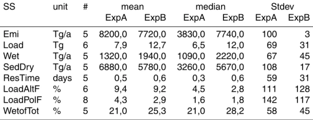
Table 2. Statistics of models results for SS: emissions, burdens, mass fractions above 5 km height, mass fractions in polar regions (south of 80 S and north of 80 N), tropospheric resi-dence times, split of removal pathways (mass fraction of wet removal in relation to total re-moval). Shown are the means, medians and the model diversities for all species in AeroCom experiments A and B.

SS unit # mean median Stdev

Load Tg 6 7,9 12,7 6,5 12,0 69 31

Wet Tg/a 5 1320,0 1940,0 1090,0 2220,0 67 45 SedDry Tg/a 5 6880,0 5780,0 3260,0 5670,0 108 17

ResTime days 5 0,5 0,6 0,3 0,6 59 31

LoadAltF % 6 9,4 9,2 4,5 2,8 111 128

LoadPolF % 8 4,3 2,9 1,6 1,8 142 117

WetofTot % 5 21,0 25,3 21,0 28,2 58 45

(17)

ACPD

7, 1699–1723, 2007

modeling

C. Textor et al.

Title Page

Tables Figures

◭ ◮

Back Close

Full Screen / Esc

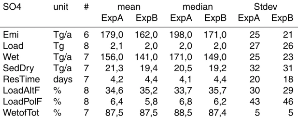
Table 3. Statistics of models results for SO4: emissions, burdens, mass fractions above 5 km height, mass fractions in polar regions (south of 80 S and north of 80 N), tropospheric residence times, split of removal pathways (mass fraction of wet removal in relation to total removal). Shown are the means, medians and the model diversities for all species in AeroCom experiments A and B.

SO4 unit # mean median Stdev

Load Tg 8 2,1 2,0 2,0 2,0 27 26

ResTime days 7 4,2 4,4 4,1 4,4 20 18

LoadAltF % 8 34,6 35,2 33,7 35,7 30 29

LoadPolF % 8 6,4 5,8 6,8 6,2 43 46

WetofTot % 7 87,5 87,5 88,5 87,4 5 5

(18)

ACPD

7, 1699–1723, 2007

modeling

C. Textor et al.

Title Page

Tables Figures

◭ ◮

Back Close

Full Screen / Esc

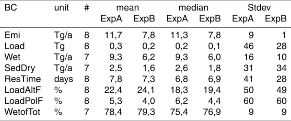
Table 4. Statistics of models results for BC: emissions, burdens, mass fractions above 5 km height, mass fractions in polar regions (south of 80 S and north of 80 N), tropospheric resi-dence times, split of removal pathways (mass fraction of wet removal in relation to total re-moval). Shown are the means, medians and the model diversities for all species in AeroCom experiments A and B.

BC unit # mean median Stdev

ExpA ExpB ExpA ExpB ExpA ExpB

Emi Tg/a 8 11,7 7,8 11,3 7,8 9 1

Load Tg 8 0,3 0,2 0,2 0,1 46 28

Wet Tg/a 7 9,3 6,2 9,3 6,0 16 10

SedDry Tg/a 7 2,5 1,6 2,6 1,8 31 34

ResTime days 8 7,8 7,3 6,8 6,9 41 28

LoadAltF % 8 22,4 24,1 18,3 19,4 50 49

LoadPolF % 8 5,3 4,0 6,2 4,4 60 60

WetofTot % 7 78,4 79,3 75,4 76,9 9 9

(19)

ACPD

7, 1699–1723, 2007

modeling

C. Textor et al.

Title Page

Tables Figures

◭ ◮

Back Close

Full Screen / Esc

Table 5. Statistics of models results for POM: emissions, burdens, mass fractions above 5 km height, mass fractions in polar regions (south of 80 S and north of 80 N), tropospheric residence times, split of removal pathways (mass fraction of wet removal in relation to total removal). Shown are the means, medians and the model diversities for all species in AeroCom experiments A and B.

POM unit # mean median Stdev

ExpA ExpB ExpA ExpB ExpA ExpB

Emi Tg/a 8 93,6 66,6 88,7 66,9 28 1

Load Tg 8 1,7 1,2 1,6 1,2 23 20

Wet Tg/a 7 79,2 53,0 74,5 52,7 32 10

SedDry Tg/a 7 19,7 13,1 18,7 13,9 23 34

ResTime days 8 7,0 6,7 7,0 6,4 30 21

LoadAltF % 8 22,3 23,8 18,3 19,7 53 49

LoadPolF % 8 3,7 3,2 4,6 3,4 62 61

WetofTot % 7 78,8 80,1 77,4 79,1 9 9

(20)

ACPD

7, 1699–1723, 2007

modeling

C. Textor et al.

Title Page

Tables Figures

◭ ◮

Back Close

Full Screen / Esc

Table 6. Statistics of models results for AER: emissions, burdens, mass fractions above 5 km height, mass fractions in polar regions (south of 80 S and north of 80 N), tropospheric resi-dence times, split of removal pathways (mass fraction of wet removal in relation to total re-moval). Shown are the means, medians and the model diversities for all species in AeroCom experiments A and B.

AER unit # mean median Stdev

ExpA ExpB ExpA ExpB ExpA ExpB Emi Tg/a 5 10 100,0 9590,0 5930,0 9680,0 79 3

Load Tg 6 35,8 36,2 36,7 37,7 18 16

ResTime days 5 1,9 1,4 1,7 1,4 61 17

LoadAltF % 6 15,3 14,5 12,4 11,2 54 62

LoadPolF % 8 2,7 2,2 1,7 1,5 96 97

WetofTot % 5 24,9 27,3 26,3 30,0 43 42

(21)

ACPD

7, 1699–1723, 2007

modeling

C. Textor et al.

Title Page

Tables Figures

◭ ◮

Back Close

Full Screen / Esc

Table 7. Model average relative changes of parameters between ExpA and ExpB expressed as (ExpB-ExpA)/ExpA in [%] for emissions, load, residence time, and fraction of wet deposition in relation to total deposition.

Emi [Tg/a] Load [Tg] ResTime [days] WetofTot [%] Mean Median Mean Median Mean Median Mean Median DUST 8.6 3.0 –1.7 –3.7 –7.7 –9.9 –11.3 –0.9 SS 76.6 95.7 88.2 64.4 26.6 4.4 37.5 20.0

SO4 –8.3 –7.4 –4.2 0.2 4.7 5.7 –0.0 0.1

BC –33.2 –30.8 –34.9 –32.8 –2.5 –1.2 1.2 0.7 POM –23.1 –18.5 –26.7 –29.3 –0.1 7.4 1.6 2.2

AER 37.8 60.9 8.1 3.1 –1.1 –35.9 18.4 5.9

(22)

ACPD

7, 1699–1723, 2007

modeling

C. Textor et al.

Title Page

Tables Figures

◭ ◮

Back Close

Full Screen / Esc

(a) 7 DUST 6 SS 8 SO4 8 BC 8 POM 6 AER # models

21 69 27 46 23 18 Diversity

-100 -60 -20 20 60 100

[%]

130 110

(b) 7 DUST 6 SS 8 SO4 8 BC 8 POM 6 AER # models

21 31 26 28 20 16 Diversity

-100 -60 -20 20 60 100

[%]

Fig. 1. Model diversities of the global, annual average aerosol burden of the five aerosol species in(a)ExpA and(b)ExpB. The diversities are indicated by gray boxes (“div”=normalized standard deviation). The individual models’ deviations from the all-models-averages are plotted as pink lines (‘data”), or as numbers if they are outside the scale of the plot. The all-models-averages are indicated by a black star (at 0%) and the medians by a black line (i.e., deviation of the median from the all-models-average). The numbers of models included in the calculation of this statistics are shown in blue below the x-axis.

(23)

ACPD

7, 1699–1723, 2007

modeling

C. Textor et al.

Title Page Abstract Introduction Conclusions References Tables Figures ◭ ◮ ◭ ◮ Back Close

Full Screen / Esc

(a)

18

ARQM ARQMB DLR DLRB GISS GISSB KYU KYUB LOA LOAB LSCE LSCEB MATCH MATCHB MOZGN MOZGNB UIOCTM UIOCTMB UIOGCM UIOGCMB ULAQ ULAQB UMI UMIB

0 1 2 3 4 5 6 7 8 9 10 11 12 0

Fraction of total [%]

0 1 2 3 4 5 6 7 8 9 10 11 12 0 (b)

0 10 20 30 40 50 60 0

Fig. 2. (a)Global, annual average mass fractions in [%] of total mass in polar regions (south of 80 S and north of 80 N) for the AeroCom models.(b)Global, annual average mass fractions in [%] of total mass above 5 km altitude for the AeroCom models. The gray shadings frame the range for each model.

(24)

ACPD

7, 1699–1723, 2007

modeling

C. Textor et al.

Title Page

Tables Figures

◭ ◮

Back Close

Full Screen / Esc

(a)

11 11 15 11

0 1 2 3 4 5 6 7 8 9 10

[days]

(b)

138

GISS LSCE MATCH MOZGN UIOCTM UIOGCM ULAQ UMI -100

-80 -60 -40 -20 0 20 40 60 80 100

(ExpB-ExpA)/ExpA [%]

Fig. 3. Tropospheric residence times in ExpA and ExpB in [days], (b)Relative changes be-tween ExpA and B expressed as (ExpB-ExpA)/ExpA in [%].

(25)

ACPD

7, 1699–1723, 2007

modeling

C. Textor et al.

Title Page Abstract Introduction Conclusions References Tables Figures ◭ ◮ ◭ ◮ Back Close

Full Screen / Esc

(a)

0 10 20 30 40 50 60 70 80 90 100 0

0 10 20 30 40 50 60 70 80 90 100 0 (b)

0 10 20 30 40 50 60 70 80 90 100 0

Fig. 4. Contribution of the individual removal processes to the total sink mass flux (annually and globally averaged) for the AeroCom models for(a) SO4 and(b) SS. The color code is given in the legend. Wet refers to wet deposition. If possible we show the individual dry sink rate coefficients (Tur: turbulent deposition, and Sed: sedimentation), otherwise the sum of the two processes (Dry=SedTur) is plotted.