Atmos. Chem. Phys., 14, 10845–10895, 2014 www.atmos-chem-phys.net/14/10845/2014/ doi:10.5194/acp-14-10845-2014
© Author(s) 2014. CC Attribution 3.0 License.
The AeroCom evaluation and intercomparison of organic aerosol in
global models
K. Tsigaridis1,2, N. Daskalakis3,4, M. Kanakidou3, P. J. Adams5,6, P. Artaxo7, R. Bahadur8, Y. Balkanski9, S. E. Bauer1,2, N. Bellouin10,a, A. Benedetti11, T. Bergman12, T. K. Berntsen13,14, J. P. Beukes15, H. Bian16, K. S. Carslaw17, M. Chin18, G. Curci19, T. Diehl18,20, R. C. Easter21, S. J. Ghan21, S. L. Gong22, A. Hodzic23, C. R. Hoyle24,25, T. Iversen11,26,13, S. Jathar5, J. L. Jimenez27, J. W. Kaiser28,11,29, A. Kirkevåg26, D. Koch1,2,b, H. Kokkola12, Y. H Lee5,c, G. Lin30, X. Liu21,d, G. Luo31, X. Ma32,e, G. W. Mann33,34, N. Mihalopoulos3,
J.-J. Morcrette11, J.-F. Müller35, G. Myhre14, S. Myriokefalitakis3,4, N. L. Ng36, D. O’Donnell37,f, J. E. Penner30, L. Pozzoli38, K. J. Pringle39,29, L. M. Russell9, M. Schulz26, J. Sciare9, Ø. Seland26, D. T. Shindell2,1,g, S. Sillman30, R. B. Skeie14, D. Spracklen17, T. Stavrakou35, S. D. Steenrod20, T. Takemura40, P. Tiitta15,41, S. Tilmes23, H. Tost42, T. van Noije43, P. G. van Zyl15, K. von Salzen32, F. Yu31, Z. Wang44, Z. Wang45, R. A. Zaveri21, H. Zhang44, K. Zhang21,37, Q. Zhang46, and X. Zhang45
1Center for Climate Systems Research, Columbia University, New York, NY, USA 2NASA Goddard Institute for Space Studies, New York, NY, USA
3Environmental Chemical Processes Laboratory, Department of Chemistry, University of Crete, Heraklion, Greece 4Institute of Chemical Engineering, Foundation for Research and Technology Hellas (ICE-HT FORTH), Patras, Greece 5Department of Civil and Environmental Engineering, Carnegie Mellon University, Pittsburgh, PA, USA
6Department of Engineering and Public Policy, Carnegie Mellon University, Pittsburgh, PA, USA 7University of São Paulo, Department of Applied Physics, Brazil
8Scripps Institution of Oceanography, University of California San Diego, CA, USA 9Laboratoire des Sciences du Climat et de l’Environnement, Gif-sur-Yvette, France 10Met Office Hadley Centre, Exeter, UK
11ECMWF, Reading, UK
12Finnish Meteorological Institute, Kuopio, Finland
13University of Oslo, Department of Geosciences, Oslo, Norway
14Center for International Climate and Environmental Research – Oslo (CICERO), Oslo, Norway 15Environmental Sciences and Management, North-West University, Potchefstroom, South Africa 16University of Maryland, Joint Center for Environmental Technology, Baltimore County, MD, USA 17School of Earth and Environment, University of Leeds, Leeds, UK
18NASA Goddard Space Flight Center, Greenbelt, MD, USA 19Department of Physics CETEMPS, University of L’Aquila, Italy 20Universities Space Research Association, Greenbelt, MD, USA 21Pacific Northwest National Laboratory; Richland, WA, USA
22Air Quality Research Branch, Meteorological Service of Canada, Toronto, Ontario, Canada 23National Center for Atmospheric Research, Boulder, CO, USA
24Paul Scherrer Institute, Villigen, Switzerland
25Swiss Federal Institute for Forest Snow and Landscape Research (WSL) – Institute for Snow and Avalanche Research (SLF), Davos, Switzerland
26Norwegian Meteorological Institute, Oslo, Norway
27University of Colorado, Department of Chemistry & Biochemistry, Boulder, CO, USA 28King’s College London, Department of Geography, London, UK
29Department of Atmospheric Chemistry, Max Planck Institute for Chemistry, Mainz, Germany
32Environment Canada, Victoria, Canada
33National Centre for Atmospheric Science, University of Leeds, Leeds, UK 34School of Earth and Environment, University of Leeds, Leeds, UK 35Belgian Institute for Space Aeronomy, Brussels, Belgium
36School of Chemical and Biomolecular Engineering and School of Earth and Atmospheric Sciences, Georgia Institute of Technology, Atlanta, GA, USA
37Max Planck Institute for Meteorology, Hamburg, Germany
38Eurasia Institute of Earth Sciences, Istanbul Technical University, Turkey
39Institute for Climate and Atmospheric Science, School or Earth and Environment, University of Leeds, Leeds, UK 40Research Institute for Applied Mechanics, Kyushu University, Fukuoka, Japan
41Fine Particle and Aerosol Technology Laboratory, Department of Environmental Science, University of Eastern Finland, Kuopio, Finland
42Institute for Atmospheric Physics, Johannes Gutenberg University, Mainz, Germany 43Royal Netherlands Meteorological Institute (KNMI), De Bilt, the Netherlands
44Laboratory for Climate Studies, Climate Center, China Meteorological Administration, Beijing, China 45Chinese Academy of Meteorological Sciences, Beijing, China
46Department of Environmental Toxicology, University of California, Davis, CA, USA anow at: Department of Meteorology, University of Reading, Reading, UK
bnow at: Department of Energy, Office of Biological and Environmental Research, Washington, DC, USA
cnow at: Center for Climate Systems Research, Columbia University, New York, NY, USA and NASA Goddard Institute for Space Studies, New York, NY, USA
dnow at: University of Wyoming, Department of Atmospheric Science, Laramie, WY, USA enow at: State University of New York, Department of Atmospheric Science, Albany, NY, USA fnow at: Finnish Meteorological Institute, Helsinki, Finland
gnow at: Nicholas School of the Environment, Duke University, Durham, NC, USA
Correspondence to:K. Tsigaridis ([email protected]) and M. Kanakidou ([email protected])
Received: 11 February 2014 – Published in Atmos. Chem. Phys. Discuss.: 7 March 2014 Revised: 3 September 2014 – Accepted: 3 September 2014 – Published: 15 October 2014
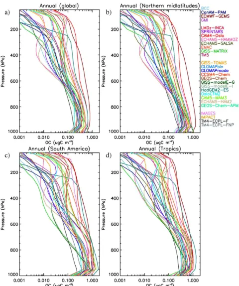
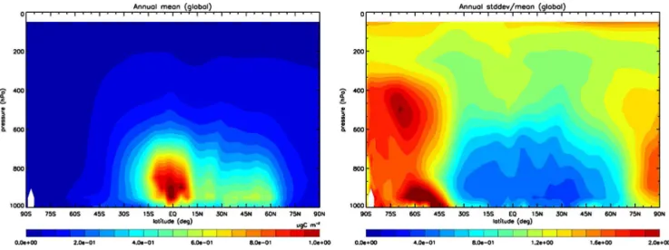
Abstract. This paper evaluates the current status of global modeling of the organic aerosol (OA) in the troposphere and analyzes the differences between models as well as between models and observations. Thirty-one global chemistry trans-port models (CTMs) and general circulation models (GCMs) have participated in this intercomparison, in the framework of AeroCom phase II. The simulation of OA varies greatly between models in terms of the magnitude of primary emis-sions, secondary OA (SOA) formation, the number of OA species used (2 to 62), the complexity of OA parameter-izations (gas-particle partitioning, chemical aging, multi-phase chemistry, aerosol microphysics), and the OA phys-ical, chemical and optical properties. The diversity of the global OA simulation results has increased since earlier Ae-roCom experiments, mainly due to the increasing complexity of the SOA parameterization in models, and the implementa-tion of new, highly uncertain, OA sources. Diversity of over one order of magnitude exists in the modeled vertical dis-tribution of OA concentrations that deserves a dedicated fu-ture study. Furthermore, although the OA / OC ratio depends on OA sources and atmospheric processing, and is important
for model evaluation against OA and OC observations, it is resolved only by a few global models.
The median global primary OA (POA) source strength is 56 Tg a−1 (range 34–144 Tg a−1) and the median SOA
source strength (natural and anthropogenic) is 19 Tg a−1 (range 13–121 Tg a−1). Among the models that take into ac-count the semi-volatile SOA nature, the median source is cal-culated to be 51 Tg a−1(range 16–121 Tg a−1), much larger
than the median value of the models that calculate SOA in a more simplistic way (19 Tg a−1; range 13–20 Tg a−1, with
one model at 37 Tg a−1). The median atmospheric burden of
OA is 1.4 Tg (24 models in the range of 0.6–2.0 Tg and 4 be-tween 2.0 and 3.8 Tg), with a median OA lifetime of 5.4 days (range 3.8–9.6 days). In models that reported both OA and sulfate burdens, the median value of the OA/sulfate burden ratio is calculated to be 0.77; 13 models calculate a ratio lower than 1, and 9 models higher than 1. For 26 models that reported OA deposition fluxes, the median wet removal is 70 Tg a−1(range 28–209 Tg a−1), which is on average 85 %
of the total OA deposition.
K. Tsigaridis et al.: The AeroCom evaluation and intercomparison of organic aerosol 10847 campaigns have been used for model evaluation. At urban
locations, the model–observation comparison indicates miss-ing knowledge on anthropogenic OA sources, both strength and seasonality. The combined model–measurements analy-sis suggests the existence of increased OA levels during sum-mer due to biogenic SOA formation over large areas of the USA that can be of the same order of magnitude as the POA, even at urban locations, and contribute to the measured urban seasonal pattern.
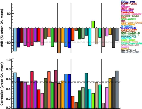
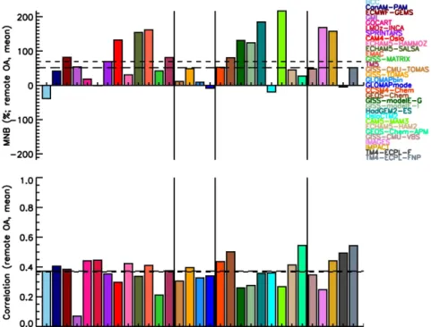
Global models are able to simulate the high secondary character of OA observed in the atmosphere as a result of SOA formation and POA aging, although the amount of OA present in the atmosphere remains largely underestimated, with a mean normalized bias (MNB) equal to−0.62 (−0.51)
based on the comparison against OC (OA) urban data of all models at the surface,−0.15 (+0.51) when compared with
remote measurements, and−0.30 for marine locations with
OC data. The mean temporal correlations across all stations are low when compared with OC (OA) measurements: 0.47 (0.52) for urban stations, 0.39 (0.37) for remote stations, and 0.25 for marine stations with OC data. The combination of high (negative) MNB and higher correlation at urban stations when compared with the low MNB and lower correlation at remote sites suggests that knowledge about the processes that govern aerosol processing, transport and removal, on top of their sources, is important at the remote stations. There is no clear change in model skill with increasing model complexity with regard to OC or OA mass concentration. However, the complexity is needed in models in order to distinguish be-tween anthropogenic and natural OA as needed for climate mitigation, and to calculate the impact of OA on climate ac-curately.
1 Introduction
Atmospheric aerosols are important drivers of air quality and climate. The organic component of aerosols can contribute 30–70 % of the total submicron dry aerosol mass, depending on location and atmospheric conditions (Kanakidou et al., 2005; Murphy et al., 2006). The majority of fine aerosol mass (PM1: particulate matter of dry diameter smaller than 1 µm) consists of non-refractory material, and has been found to contain large amounts of organic matter (Zhang et al., 2007; Jimenez et al., 2009), as measured by the Aerosol Mass Spec-trometer (AMS).
Global model estimates of the dry organic aerosol (OA) direct radiative forcing at the top of the atmosphere are
−0.14±0.05 W m−2 based on AeroCom phase I
experi-ments (Schulz et al., 2006), which was decomposed dur-ing AeroCom phase II to −0.03±0.01 W m−2 for
pri-mary organic aerosol (POA) from fossil fuel and biofuel,
−0.02±0.09 W m−2 for secondary organic aerosol (SOA)
and 0.00±0.05 W m−2 for the combined OA and black
carbon from biomass burning (Myhre et al., 2013). IPCC (2013) assessed the contribution of anthropogenic primary and secondary organic aerosols to the radiative forcing from aerosol–radiation interactions (RFari) to be −0.12 (−0.4
to+0.1) W m−2. Spracklen et al. (2011) estimated the
cli-mate forcing of the anthropogenically driven natural SOA alone (including the presence of water on hydrophilic OA) at−0.26±0.15 W m−2(direct effect) and−0.6+−00..2414W m−2
(indirect effect). These amounts largely depend on the atmo-spheric loadings of OA simulated by the models under past, present and future climate conditions, and on the properties they attribute to them. Indeed, Myhre et al. (2013) calculated a SOA load of 0.33±0.32 Tg, while Spracklen et al. (2011)
estimated a SOA load of 1.84 Tg, which resulted in an order of magnitude higher radiative forcing. There is therefore an urgent need for a consensus between models and agreement with observations, in order to constrain the large variability between models and, consequently, the OA impact on cli-mate.
1.1 Definitions
absorption and the ability to act as cloud condensation nu-clei (CCN). Therefore, the ratio of OA to OC mass (Turpin and Lim, 2001; Aiken et al., 2008) requires careful investi-gation. Furthermore, OA compounds differ in their volatility, solubility, hygroscopicity, chemical reactivity and their phys-ical and optphys-ical properties. Due to the chemphys-ical complexity of the organic component of aerosols (Goldstein and Gal-bally, 2007), only simplified representations are introduced in global chemistry climate models (Kanakidou et al., 2005; Hallquist et al., 2009). As a compromise between simplicity and accuracy, the net effect of the complex mixture of OA is described by only a limited number of representative com-pounds or surrogates.
1.2 Sources
Kanakidou et al. (2005) reviewed how organic aerosols were incorporated into global chemistry transport models (CTMs) and general circulation models (GCMs), and identified gaps in knowledge that deserved further investigation. The POA sources include fossil fuel, biofuel and biomass burning, as well as the less understood sources of marine OA, bi-ological particles and soil organic matter on dust (Kanaki-dou et al., 2012, and references therein). Biogenic VOCs (BVOCs) greatly contribute to OA formation (e.g., Griffin et al., 1999b; Kanakidou et al., 2012), implying that sig-nificant feedbacks exist between the biosphere, the sphere and climate that affect the OA levels in the atmo-sphere, which was also demonstrated by more recent stud-ies (Tsigaridis et al., 2005; Arneth et al., 2010; Carslaw et al., 2010; Paasonen et al., 2013). In addition, oxidant and pollutant enhancement by human-induced emissions is ex-pected to increase OA levels, even those chemically formed by BVOC (Hoyle et al., 2011, and references therein); it is therefore conceivable that some portion of the ambient bio-genic SOA, which would had been absent under preindus-trial conditions, can be removed by controlling emissions of anthropogenic pollutants (Carlton et al., 2010). Goldstein and Galbally (2007) estimated that SOA formation could be as high as 910 TgC a−1, which is at least an order of
mag-nitude higher than any SOA formation modeling study, as shown here. Spracklen et al. (2011) were able to reconcile AMS observations (mostly from the Northern Hemisphere mid-latitudes during summer) with global CTM simulations by estimating a large SOA source (140 Tg a−1). 100 Tg a−1
was characterized as anthropogenically controlled, 90 % of which was possibly linked to anthropogenically enhanced SOA formation from BVOC oxidation. Similar conclusions were reached by Heald et al. (2011) by comparing aircraft AMS observations of submicron OA with the results of an-other global model, and by Heald et al. (2010) by account-ing for the satellite-measured aerosol optical depth that could possibly be due to OA. Recently, Carlton and Turpin (2013) showed that anthropogenically enhanced aerosol water in the eastern USA could lead to an increase in WSOC from
BVOC. Although large uncertainties still exist in SOA mod-eling, there is a need for models to document and improve treatments of solubility, hygroscopicity, volatility and optical properties of the OA from different sources. The SOA for-mation from anthropogenic VOCs, despite a recent estimate of 13.5 Tg a−1that makes it a non-negligible SOA source in polluted regions (De Gouw and Jimenez, 2009), is frequently neglected by global models.
1.3 Atmospheric processing
K. Tsigaridis et al.: The AeroCom evaluation and intercomparison of organic aerosol 10849 has been successfully used to simulate the evolution of OA in
field campaigns (Murphy et al., 2011, 2012). Unfortunately, this new approach needs an even larger number of tracers, which makes it extremely difficult to implement in a global climate model without a large performance penalty. Still, it certainly adds value to our OA understanding, since the ratio of organic aerosol mass (OA) to organic carbon (OA / OC), an alternative way to describe the degree of oxidation of OA, does greatly vary in time and space (Turpin and Lim, 2001). This variability is either neglected or taken into account in a very simplistic way in models.
Yu (2011) extended the two-product SOA formation scheme in the GEOS-Chem model by taking into account the volatility changes of secondary organic gases arising from the oxidative aging process (Jimenez et al., 2009) as well as the kinetic condensation of low-volatility secondary or-ganic gases. It was shown that, over many parts of the con-tinents, low-volatility secondary organic gas concentrations are generally a factor of∼2–20 higher than those of sulfuric
acid gas, and the kinetic condensation of low-volatility sec-ondary organic gases significantly enhances particle growth rates. Based on this computationally efficient new SOA for-mation scheme, annual mean SOA mass concentrations in many parts of the boundary layer increase by a factor of 2–10, in better agreement with Aerosol Mass Spectrometer (AMS) SOA measurements (Yu, 2011).
Hallquist et al. (2009) also summarized new laboratory data that provided insight into the chemical reaction path-ways for the formation of oligomers and other higher molec-ular weight products observed in SOA. They determined higher production rates of SOA from their precursors’ oxi-dation than earlier measurement studies and linked the de-pendence of SOA yield from VOC oxidation to the oxidant levels. In chamber experiments, Volkamer et al. (2009) have shown that even small (C2)molecules undergoing
aqueous-phase reactions can produce low-volatility material and con-tribute to SOA formation in the atmosphere, a process that was reviewed by Ervens et al. (2011) and Lim et al. (2013). The global modeling study of Myriokefalitakis et al. (2011) has shown that multiphase reactions of organics significantly increase the OA mass (5–9 % when expressed as OC) and its oxygen content, while Murphy et al. (2012) suggested that these reactions are not enough to explain the observed O / C content of OA.
1.4 Losses
Hallquist et al. (2009) used the VBS concept and estimated the atmospheric deposition of OA to be 150 Tg a−1, higher than earlier estimates and similar to the total particulate OC deposition of 147 Tg a−1(109 Tg a−1of WSOC) calculated by Kanakidou et al. (2012). Dry and wet removal of organic vapors that are in thermodynamic equilibrium with SOA be-comes increasingly important with atmospheric processing (Hodzic et al., 2013) and was found to lead to 10–30 % (up
to 50 %) removal of anthropogenic (biogenic) SOA (Hodzic et al., 2014). Volatilization of OA upon heterogeneous oxida-tion has been observed for laboratory and ambient particles (George and Abbatt, 2010) and might be a significant OA sink (Heald et al., 2011).
1.5 Motivation and aim
During the AeroCom phase I modeling experiments (Textor et al., 2006), although most of the models considered both primary and secondary OA sources, OA was simulated in a very simplified way in which both primary and secondary OA were treated as non-volatile. OA was only allowed to age via hydrophobic-to-hydrophilic conversion, and was re-moved from the atmosphere by particle deposition. Compar-isons of individual models with OA observations have shown a large underestimation of the organic aerosol component by models, especially in polluted areas (Volkamer et al., 2006, and references therein). They showed that the underestima-tion of SOA by models increases with photochemical age, which can be partially correlated with long-range transport, with the largest discrepancies in the free troposphere, sug-gesting missing sources or underestimated atmospheric pro-cessing of organics in models.
Several global models now treat SOA as semi-volatile, as detailed below, which enables potentially more accu-rate model calculations. Some models also account for intermediate-volatility organics, multiphase chemistry and semi-volatile POA (e.g., Pye and Seinfeld, 2010; Jathar et al., 2011; Myriokefalitakis et al., 2011; Lin et al., 2012), with encouraging results in reducing the difference between mod-els and observations. Indeed, the modeled SOA concentra-tions in Mexico City were much closer to observaconcentra-tions when intermediate-volatility organics were taken into account in a regional model, although it was unclear if the model– observation gap was reduced for the right reasons (Hodzic et al., 2010). However, OA simulations have many degrees of freedom due to incomplete knowledge of the behavior and fate of OA in the troposphere. Thus, several assump-tions made are translated to model tuning parameters that vary greatly between models.
1.6 Terminology
In atmospheric OA research, several naming conventions and abbreviations are used, often ambiguously and inconsistently between authors. To avoid confusion, we clarify here the conventions adopted in this paper, which we use through-out. Note that some aspects of our terminology are differ-ent from the very recdiffer-ent VBS-cdiffer-entered attempt by Murphy et al. (2014) to clarify this ambiguity systematically; new model development is required from modelers to adopt the new naming convention in future model simulations.
– Organic aerosol (OA) and the main OA components, i.e., primary and secondary OA (POA and SOA, respec-tively): we use these terms to refer to the total mass that organic compounds have in the aerosol phase, including H and O, and potentially other elements like N, S and P. Other authors have used the term organic matter (OM), which is synonymous with our OA definition. The units used are µg m−3for surface mass concentrations at
am-bient conditions and Tg for burden and budget calcu-lations. OA amounts exclude the water associated with it (assuming that OA is hygroscopic), an important ad-ditional component that affects particle size, refractive index and light scattering efficiency.
– Organic carbon (OC), together with other OC compo-nents, like, e.g., primary and secondary OC (POC and SOC, respectively): these terms refer to the mass of car-bon present in OA, instead of to the total OA mass. The units used here are µgC m−3 for surface mass
concen-trations. This is typically the terminology that is used when comparing model results with filter measurements analyzed by thermal–optical methods.
OA mass can increase for constant OC, due to oxidative ag-ing; this is something that very few models calculate, and should be improved in the future. The OA / OC ratio is dis-cussed in more detail in Sect. 1.7. Care should also be taken for the case of methane sulfonic acid (MSA), since the letter A stands for “acid”, not “aerosol”, as in OA. When reporting MSA results, we refer to the total methane sulfonic acid mass present in OA and not its carbon mass only, unless clearly stated otherwise.
1.7 OA / OC and O / C ratios
To calculate the total organic aerosol mass concentration for each model, we apply the following equation:
OAi=OCi∗(OA/OC)i (1)
where (OA / OC)iis the organic aerosol to organic carbon ra-tio for aerosol traceri(Table 1). OA / OC, frequently termed
as OM / OC in the literature (OM: organic matter), was found to correlate extremely well with the O / C ratio in Mexico City and chamber data (Aiken et al., 2008), because of low
N / C ratios. A low OA / OC ratio is also indicative of “fresh” OA as deduced from observations (Turpin and Lim, 2001; Philip et al., 2014). The OA / OC ratio varies greatly between models, with many of them setting OA / OC=1.4 as a
con-stant for all OA sources. Some models use different OA / OC ratios for every OA tracer: IMAGES, IMPACT, and the two TM4-ECPL models calculate the specific OA / OC ratio for each of their aerosol tracers, depending on their sources and chemical identity. CAM4-Oslo uses 1.4 for fossil fuel and biofuel, OsloCTM2 and SPRINTARS use 1.6, while all three models use 2.6 for biomass burning. In the case of CAM4-Oslo and SPRINTARS, it is not possible to calculate the OC concentration from the model fields accurately, since they only track one tracer. For this, we used a single value, that of the fossil fuel each model is using, which will lead to an underestimation of their OC concentration (but not of OA) close to biomass burning sources. The remaining mod-els use a constant OA / OC ratio: Chem and GEOS-Chem-APM use a specified value of 2.1, GISS-CMU-VBS and GISS-CMU-TOMAS use 1.8, and all other models use 1.4. Observations (Turpin and Lim, 2001; Aiken et al., 2008) suggest that OA / OC values of 1.6±0.2 and 2.1±0.2 are
good approximations for urban and non-urban aerosols, re-spectively, indicating that most models might use OA / OC values that are low. The study of both the OA / OC and O / C ratios is extremely important and warrants a dedicated inves-tigation; although this will be mentioned in the present work, it will be studied in detail in the future.
1.8 Organic aerosol speciation
In the present work, we have separated organic aerosols into five categories, as described below and summarized in Ta-ble 1. The models are then grouped based on their OA pa-rameterizations in Table 2.
K. Tsigaridis et al.: The AeroCom evaluation and intercomparison of organic aerosol 10851 emissions, emitted in the gas phase) with a chemical
lifetime of 12 h that forms a non-volatile SOA tracer (which is included in tPOA). In GISS-TOMAS the SOA precursor emissions are based on terpenes, with a 10 % yield, while a-pinene oxidation by all major
oxidants (OH, O3, NO3) produces non-volatile SOA
(included in tPOA) with a 13 % yield in GLOMAPbin and GLOMAPmode. SPRINTARS has a 9.2 % yield of non-volatile SOA (Griffin et al., 1999a, b) from monoterpene emissions, and considers this tracer as inert and tracks it separately, in contrast to the other models that produce non-volatile SOA and track it together with tPOA. SOA from anthropogenic VOCs is included in only a few models, and is not included in tPOA.
2. mPOA, for primary organic aerosol from marine sources. CAM4-Oslo has a primary marine organic source of 8 Tg a−1 (Spracklen et al., 2008) with the
same emissions distribution as sea salt (provided by Dentener et al., 2006) included in tPOA. IMPACT includes a mPOA source of 35 Tg a−1 (Gantt et al.,
2009a), which scales with chlorophyll a and sea salt
as a proxy of marine biological activity (O’Dowd et al., 2004), while GISS-modelE-G/I and TM4-ECPL-F/FNP include a similar source of submicron mPOA based on Vignati et al. (2010). The GISS-modelE-G/I source is described in Tsigaridis et al. (2013) and the TM4-ECPL-F/FNP mPOA source in Myriokefalitakis et al. (2010). It has to be noted that these two stud-ies have a factor of 10 difference in submicron mPOA source strength, despite having very similar source function parameterizations. This results from differ-ences in sea-spray size distribution assumptions, as dis-cussed in Tsigaridis et al. (2013). In addition to the fine-mode mPOA source, TM4-ECPL-FNP accounts for about 30 TgC a−1of coarse-mode mPOA
(Kanaki-dou et al., 2012), but that was not taken into account in the present study, since all measurements used here are for fine aerosols.
3. trSOA, for “traditional” secondary organic aerosol, which is produced by gas to particle mass transfer of secondary organic material, either assuming the mate-rial has a finite vapor pressure (a gas-particle partition-ing process) or that it has zero vapor pressure (a conden-sation process). The most common precursors of SOA used across models are isoprene and terpenes, although few models have other precursors as well, as presented in Sect. 2. All models have some form of trSOA, either included in tPOA (as explained above), or via an ex-plicit treatment of the semi-volatile oxidation products of the precursor VOCs. For the models other than the ones presented in (a) above that treat SOA as part of tPOA, the approach used and species taken into account differ. CAM5-MAM3 prescribes mass yields from 5
trSOA precursor categories (isoprene, terpenes, aro-matics, higher molecular weight alkanes and alkenes, with yields of 6.0, 37.5, 22.5, 7.5, and 7.5 %, respec-tively), which then reversibly and kinetically partition to the aerosol phase. GISS-CMU-VBS uses the volatility-basis set, but without aging for the biogenic trSOA. The rest of the models use the two-product model ap-proach to calculate trSOA; see the references column in Table 3 for more details. GEOS-Chem-APM consid-ers the volatility changes of the gaseous semi-volatile compounds arising from the oxidation aging process, as well as the kinetic condensation of low-volatility gases (Yu, 2011). HadGEM2-ES does not calculate trSOA on-line; instead, it uses an offline 3-D monthly mean trSOA climatology obtained from the STOCHEM CTM (Der-went et al., 2003). The two-product model implemented in IMAGES was modified to account for the effect of water uptake on the partitioning of semi-volatile organ-ics, through activity coefficients parameterized using a detailed model for α-pinene SOA (Ceulemans et al.,
2012). IMPACT predicts semi-volatile SOA from or-ganic nitrates and peroxides using the gas-particle parti-tioning parameterization with an explicit gas-phase or-ganic chemistry. These condensed semi-volatile com-pounds are assumed to undergo further aerosol-phase reactions to form non-evaporative SOA with a fixed 1-day e-folding time (Lin et al., 2012). The two TM4-ECPL models account for SOA aging by gas-phase ox-idation by OH with a rate of 10−12cm3molec−1s−1,
while the conversion of insoluble POA to soluble is pa-rameterized as described by Tsigaridis and Kanakidou (2003) with a decay rate that depends on O3 concen-tration and water vapor availability, which corresponds to an approximately 1-day global mean turnover time, with strong spatial variability.
aerosol water (Fu et al., 2008, 2009; Stavrakou et al., 2009; Myriokefalitakis et al., 2011), with the two TM4-ECPL models having a primary glyoxal source from the oceans of 4.1 TgC a−1, which is not present in the other two models. Glyoxal and methylglyoxal are highly re-active species in the aqueous phase. The aqueous-phase reactions can occur both in aerosol water and cloud droplets; after droplet evaporation, the residual organic compounds remain in the aerosol phase in the form of OA. By applying a reactive uptake (γ ) of glyoxal
and methylglyoxal on aqueous particles and cloud drops (Liggio et al., 2005), IMAGES and IMPACT parameter-ized the irreversible surface-controlled uptake of these soluble gas-phase species. On the other hand, Myrioke-falitakis et al. (2011) applied a much more detailed aqueous-phase chemical scheme in cloud droplets in or-der to produce oxalate. For IMPACT, 52 % of the to-tal SOA comes from glyoxal and methylglyoxal mul-tiphase chemistry (Lin et al., 2012). IMPACT also in-cludes ntrSOA formation from the uptake of gas-phase epoxides onto aqueous sulfate aerosol (Paulot et al., 2009), which contributes by 25.1 Tg a−1 (21 %) to the
total SOA formation (Lin et al., 2012).
5. MSA, an oxidation product of DMS, is also a SOA com-ponent. Although a minor organic aerosol component on the global scale, MSA can be very important in re-mote oceanic regions, especially when mPOA is rela-tively low: observations indicate that MSA can be at least 10 % of the total WSOC mass (Sciare et al., 2001; Facchini et al., 2008) at marine locations. Only CAM4-Oslo, GEOS-Chem-APM, GISS-modelE-G/I, IMPACT, LMDz-INCA, TM4-ECPL-F/FNP and TM5 have this tracer, which has been typically neglected from the or-ganic aerosol budget in modeling studies. In CAM4-Oslo, MSA is included in tPOA, in IMPACT it is in-cluded in mPOA (which is in turn inin-cluded in tPOA), whereas in the other models, it is individually tracked. A summary of the OA processes included in the models is presented in Table 2. The total organic aerosol mass is calcu-lated as follows:
OA=tPOA+mPOA+trSOA+ntrSOA+MSA (2)
The models that have mPOA, SOA and/or MSA included in tPOA do not track them separately, so there is no risk of double-counting any OA species. In addition to this catego-rization, in order to compare with AMS data (see Sect. 3) we separate the modeled OA into HOA (hydrocarbon-like OA) and OOA (oxygenated OA) as defined by Zhang et al. (2005), when sufficient information on hydrophobic/hydrophilic spe-ciation from the models is available. We use the termi-nology HOA / OOA instead of water soluble/insoluble OC (WSOC / WIOC), and compare only with AMS organic aerosol data, in order to contrast with the OC measurements
that refer to organic carbon. The separation into HOA and OOA has been provided by only a few models: ECHAM5-HAM2, ECMWF-GEMS, EMAC, modelE-G, GISS-modelE-I, GISS-TOMAS, GLOMAPbin, GLOMAPmode, IMAGES, LMDz-INCA, TM4-ECPL-F, TM4-ECPL-FNP and TM5. From the AMS perspective, the total OA is cal-culated as follows:
OA=HOA+OOA (3)
Further subdivisions into other categories of OOA (Jimenez et al., 2009) are neglected in this study. In addition, the term POA used in Zhang et al. (2011) as a surrogate for different HOA categories is also not taken into account here.
2 Description of models
The models participating in the present study differ in (a) the spatial resolution, both horizontal and vertical, (b) the under-lying model with which the aerosol calculations are coupled, which can be either a CTM or a GCM, and will be named “host model” from now on, (c) the emissions used, both for POA and SOA precursors, as well as for other gaseous and aerosol tracers, (d) the inclusion or not of aerosol micro-physics, which are implemented in multiple ways (Mann et al., 2014), and (e) the OA processes simulated, i.e., the chem-ical and physchem-ical processes that change existing OA (such as oxidative aging), and the representation of SOA formation.
The complexity of the OA calculations varies greatly be-tween models (Table 3). There are differences in OA emis-sion source strength, both for primary particles (Table 4) and precursors of secondary OA (Table 5), as well as in the to-tal number of OA tracers used (2 to 62; Table 1) and their properties, especially with regard to the temperature depen-dence of their vapor pressure (Sect. 6). Although a classifi-cation is difficult, one can categorize the models in various groups when considering OA modeling from different per-spectives. The classification used here will be presented later (Sect. 1.8).
K. Tsigaridis et al.: The AeroCom evaluation and intercomparison of organic aerosol 10853 difference being in the calculation of OA: the first one uses a
bulk aerosol scheme with the VBS approach (Donahue et al., 2006; Jathar et al., 2011), and the second one the aerosol mi-crophysics scheme TOMAS (Adams and Seinfeld, 2002; Lee and Adams, 2010, 2012). Similarly, GISS-MATRIX, the two GISS-modelE models and GISS-TOMAS use the same host GCM (GISS-E2), but they have different aerosol represen-tations: GISS-MATRIX uses the aerosol microphysics mod-ule MATRIX (Bauer et al., 2008), the two modelE versions have a bulk aerosol scheme (Koch et al., 2006, 2007; Miller et al., 2006; Tsigaridis and Kanakidou, 2007; Tsigaridis et al., 2013) and GISS-TOMAS uses the same aerosol micro-physics scheme as GISS-CMU-TOMAS (Lee and Adams, 2012; Lee et al., 2014). GISS-modelE-G and GISS-modelE-I only differ in the emissions used; they both have CMIP5 an-thropogenic emissions for all tracers (Lamarque et al., 2010), but GISS-modelE-G uses GFED3 (van der Werf et al., 2010) for biomass burning. GLOMAPbin and GLOMAPmode use the same host CTM (TOMCAT; Chipperfield, 2006), with the only difference being the sectional and modal aerosol micro-physics calculations (Mann et al., 2012). TM4-ECPL-FNP is almost identical to TM4-ECPL-F, but also takes into ac-count the contribution to OA from primary biological parti-cles and soil dust in the fine and coarse modes (Kanakidou et al., 2012). These two models also use different biogenic and anthropogenic VOC emission inventories (Tables 4 and 5).
All model results presented here come from monthly mean data, while measurements are averaged in monthly mean val-ues, prior to any comparison with model data.
2.1 Meteorology
One major difference between the configurations of the mod-els is the meteorology and meteorological year used. This af-fects aerosol transport, removal, chemistry (e.g., temperature dependence of reaction rates) and gas-particle partitioning of semi-volatile species. In some models, meteorology also di-rectly affects natural aerosol emissions, like wind-driven sea salt, marine organic aerosol, dust and VOC emissions from the vegetation and oceans. Indirectly, meteorology affects MSA sources, since MSA is produced via dimethyl sulfide (DMS) oxidation, whose source is affected by wind speed and its oxidation depends on chemical rates.
Several climate models that participated in this inter-comparison calculate the meteorology online. These are BCC, CAM4-Oslo, CAM5-MAM3, CanAM-PAM, GISS-CMU-VBS and GISS-CMU-TOMAS. In addition, climate models GISS-MATRIX, G, GISS-modelE-I and SPRGISS-modelE-INTARS are nudged to the NCEP reanaly-sis (Kalnay et al., 1996), GISS-TOMAS is nudged to MERRA meteorology (Rienecker et al., 2011), HadGEM2-ES and ECHAM5-HAMMOZ are nudged to the operational ECMWF meteorology (http://www.ecmwf.int/products/data/ archive/descriptions/od), and LMDz-INCA is nudged to ECMWF reanalysis from the Integrated Forecast System.
The remaining models use a variety of prescribed meteorol-ogy data sets for the year 2006 (Table 3), except that GISS-CMU-VBS uses 2008, IMPACT uses 1997, and TM4-ECPL-FNP uses 2005.
2.2 Emissions
All participating models include POA in their simulations. The sources are both anthropogenic and biogenic, and can be classified as follows:
1. Fuel emissions. These exclusively anthropogenic sources include fossil fuel and biofuel burning. All models include these sources, but the emission inven-tories used are not always the same (Table 4). A number of models used emissions for the year 2000; others used emissions for the year 2006, and one for the year 2005 (TM4-ECPL-FNP). Cooking emissions, which can con-tribute up to 50 % of the POA in many urban areas (Mohr et al., 2012) are not included in any model. 2. Biomass burning. As in the case of fuel emissions, not
all models use the same sources or representative years. Only about half of the models use biomass burning emissions from the year 2006 (Table 4), which is the reference year in the present study. Biomass burning is the largest POA source; it has significant interannual and strong seasonal variability and is the most uncer-tain POA source on a global scale (Andreae and Mer-let, 2001), making it extremely important for compar-ison with measurements, especially at remote sites, to properly represent this source. Comparisons of several model simulations with the smoke aerosol optical depth (AOD) observed by MODIS have indicated a systematic underestimation when emissions from bottom-up inven-tories like GFED, used by several models here, are used. The underestimation may be as high as a factor of 3 on the global scale (Kaiser et al., 2012, and references therein), and strongly varies by region (Petrenko et al., 2012).
3. Marine sources. Few models take into account marine sources of organic aerosols (see Sect. 1.8); these de-pend on sea spray emissions. The GISS-modelE-G and GISS-modelE-I source depends on SeaWiFS chloro-phyllameasurements from the year 2000 (Tsigaridis et
al., 2013), while IMPACT and TM4-ECPL-F/FNP cal-culations use the MODIS chlorophylla data from the
prescribed AeroCom phase I fine-mode sea salt emis-sions (Dentener et al., 2006).
4. Other primary sources. TM4-ECPL-FNP (Kanakidou et al., 2012) includes some fine-mode POA sources that do not exist in any other global model in this intercompar-ison. These consist of primary biological particle emis-sions from plants (25 Tg a−1)and soil organic matter on
dust (0.2 Tg a−1).
5. “Pseudo” primary non-volatile SOA fluxes. A num-ber of models parameterize SOA chemical production in the atmosphere as a source of non-volatile aerosol emitted directly from vegetation. SOA is then modified similarly to POA by processes like transport, chemical aging, growth, coagulation and condensation, among others, depending on the model. BCC, CanAM-PAM, ECHAM5-HAMMOZ, ECHAM5-SALSA, ECMWF-GEMS, EMAC, GISS-CMU-TOMAS, LMDz-INCA and TM5 use a global source of 19.1 Tg a−1(Dentener
et al., 2006). This source is equivalent to a 15 % yield from the year 1990 monoterpene emissions (Guenther et al., 1995) and is identical to the source used during the AeroCom phase I experiments. GISS-CMU-TOMAS, GISS-TOMAS, GLOMAPbin and GLOMAPmode also use the same approach (based on the Guenther et al. (1995) emissions, except GISS-TOMAS, which is based on Lathière et al., 2005), but with SOA produced according to an assumed molar yield following oxida-tion (see Sect. 1.8 and Table 1), which results in a calcu-lated SOA source of 19.1, 17.1, 23.1, and 23.0 Tg a−1,
respectively. GISS-MATRIX and GISS-TOMAS use a 10 % yield (17.1 Tg a−1)from monoterpene emissions
for the year 1990 from Lathière et al. (2005), while GMI and GOCART assume a 10 % yield (12.7 Tg a−1)from
the Guenther et al. (1995) monoterpene emissions. In the case of CAM4-Oslo, the strength of the secondary source suggested by Dentener et al. (2006) has been scaled up to 37.5 Tg a−1, based on Hoyle et al. (2007). In addition to the primary aerosol emissions, the inventories used for the precursors of secondary organic aerosols are also both very diverse and of great importance. These are pre-sented in Table 5.
3 Measurements
The compilations of PM2.5OC measurements by Bahadur et al. (2009) and PM1OA measurements by Zhang et al. (2007) form the basis for the present study. Additional OC and OA observations from continuous monitoring networks and indi-vidual case studies reported in the literature have been used to increase the spatial and temporal coverage of the observa-tional database for model evaluation.
The OC measurements reported by Bahadur et al. (2009) include data from
– The Interagency Monitoring of Protected Visual En-vironments (IMPROVE; http://vista.cira.colostate.edu/ IMPROVE), which is the American monitoring network for national parks and wilderness areas, for 1988–2006. – The Speciated Trends Network (STN) administered by the Environmental Protection Agency (Air Quality Sys-tem Environmental Protection Agency (AQSEPA); http: //www.epa.gov/ttn/airs/airsaqs), which mainly consists of urban monitoring stations within the USA, for 2000– 2007.
– The North American Research Strategy for Tro-pospheric Ozone (NARSTO; http://www.narsto.org), which consists of measurements in Mexico, the USA and Canada, for 1999–2005.
– The New England Air Quality Studies (NEAQS; http: //www.esrl.noaa.gov/csd/ projects/neaqs), which con-tains measurements from the New England region, as a part of NOAA field studies, for 2002.
– The Southeastern Aerosol Research and Characteriza-tion Study (SEARCH; Hansen et al., 2003), which is a monitoring network for the southeastern United States, for 1998–2007.
– The European Monitoring and Evaluation Programme (EMEP; http://www.emep.int). EMEP is a European monitoring network with a few hundred monitoring sta-tions all over Europe; only a few measure OC, which are used here, for 2002–2006.
– The Construction, Use and Delivery of a Euro-pean Aerosol Database (CREATE; http://www.nilu.no/ projects/ccc/create). CREATE is a database that com-piles aerosol data from eight European countries, for 2000–2006.
– The Hong Kong Environmental Protection Agency (http://www.epd.gov.hk/epd/eindex.html), with mea-surements from the extended area of Hong Kong, for 2000–2002.
K. Tsigaridis et al.: The AeroCom evaluation and intercomparison of organic aerosol 10855 The IMPROVE and AQSEPA networks cover most of the
United States more than adequately. The EMEP monitoring network together with the European Integrated project on Aerosol, Cloud, Climate, and Air Quality Interactions (EU-CAARI) and CREATE data sets and other studies found in the literature provide good coverage of a large part of Eu-rope, with stations in 17 countries. Although the spatial and temporal coverage is not as extensive as in the USA, it pro-vides a comprehensive representation of different sources and chemical environments over Europe. There are limited measurements from Asia, with many of them being at ur-ban or urur-ban-influenced locations in India and China. South America, Africa and Oceania have very poor spatial and tem-poral coverage, despite the importance of the tropical forests of the former two on the global OA budget. Marine areas are almost exclusively covered by short-term measurement cam-paigns, with the exception of Amsterdam Island in the south-ern Indian Ocean (Sciare et al., 2009). All OC measurements are PM2.5or smaller sizes, e.g., PM1.8(Koulouri et al., 2008). A rapidly increasing number of AMS OA measurements has been reported in the literature since the work of Zhang et al. (2007). Most of these AMS measurements are available online, in a web page created and maintained by Q. Zhang and J.-L. Jimenez (http://tinyurl.com/ams-database). We in-clude in this analysis most of the ground-based data available as of January 2013. These data include the only AMS mea-surements so far available for a whole year (using the ACSM instrument, which is a monitoring version of the AMS; Ng et al., 2011), from Welgegund, South Africa (Tiitta et al., 2014); all other stations were measuring for about a month or less. The geographical coverage of the AMS stations is far less dense than the OC measurement locations, but the num-ber of stations is rapidly increasing. Longer records are also starting to appear in the literature (Tiitta et al., 2014), and are expected to increase in the near future. It is important to note that the OA values provided by the AMS-type instruments have uncertainties (30 %) inherent in quantifying the detec-tion efficiency for the wide range of organic molecules that make up complex SOA material (Canagaratna et al., 2007; Middlebrook et al., 2012). Care should be taken when using AMS-type OA data in models that estimate organic aerosol content.
All station data have been classified in three main cate-gories: urban, remote and marine. Urban sites are defined as those that are either in cities or highly influenced by them. AMS stations characterized as “urban downwind” fall in this category. Remote sites are defined as those not influenced by local anthropogenic activities, and include forested regions, mountains, rural areas, etc. Marine sites are all measurements from ships or from coastal stations that are highly influenced by the marine atmosphere. Only two AMS stations fall into this category (Okinawa, Japan, and Mace Head, Ireland), and for simplicity, they were classified in the “remote” category. The two databases (OC and OA measurements) have been kept separate because of the added complexity related to the
OA / OC ratio (Sect. 1.7). Almost all models calculate OA mass concentration, integrated across the fine-mode size dis-tribution where appropriate, which can be compared with AMS measurements without any unit conversion. To com-pare with filter measurements of OC, we used the models’ assumptions about the OA / OC ratio to convert the mod-eled OA to OC. As mentioned earlier, the importance of the OA / OC ratio will be explored in the future. The cutoff diam-eter of aerosols can also be an issue (Koulouri et al., 2008), but it is not expected to be significant in the present study, given the assumptions that the models adopt for the primary OA sources. No model adds fine OA mass from coarse-mode sources, and no model allows partitioning of semi-volatile gases to the coarse mode; thus, the difference between the PM2.5 filter measurements and PM1 AMS data is not ex-pected to be properly resolved by models, even if they in-clude aerosol microphysics calculations.
4 Results
4.1 Global budgets
Many global models have evolved significantly since the Ae-roCom phase I intercomparison studies. During phase I, the first experiment, AeroCom A (ExpA), was designed in a very similar way to the AeroCom phase II model simulations de-scribed here (Schulz et al., 2009). For the second, AeroCom B (ExpB), all models used the same emission inventories. The outcomes of these studies have been summarized by Textor et al. (2006) for ExpA and Textor et al. (2007) for ExpB and is compared with the present study in detail here (Fig. 1). The two AeroCom phase I studies focused on the total aerosol budget, but the individual aerosol components were also studied. Sixteen models participated in ExpA and twelve in ExpB, most of which are earlier versions of the models that participated in the present intercomparison.
The large number of models used in this study adds a sig-nificant level of complexity to the interpretation of results, due to the large diversity of inputs and configurations used by the different modeling groups. Despite the large differ-ences between model formulations, on the global scale, sev-eral interesting similarities and patterns appear, which are frequently associated with the parameterizations and emis-sion inventories used.
4.1.1 Emissions
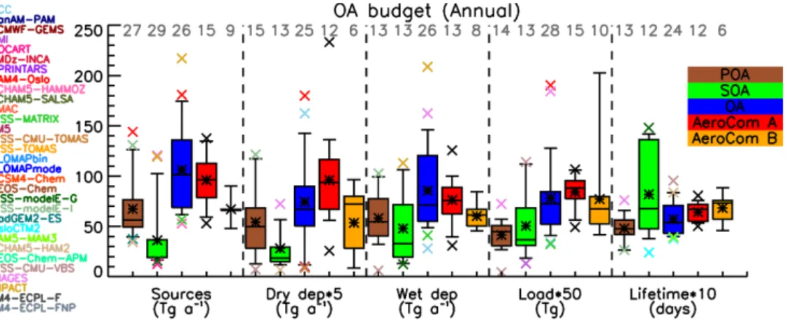
Figure 1.Box and whisker plot for all POA, SOA and OA global budgets and comparison with AeroCom phase I (Textor et al., 2006, 2007) results. The boxes represent the first and third quartile range (50 % of the data), the line is the median value, the star is the mean, and the error bars represent the 9/91 % of the data. Outliers are presented with x-symbols, with the corresponding color of the model, and the numbers of models participating in each bars statistics are presented with a grey number at the top. The AeroCom phase I outliers are presented with black color, since there is no direct correspondence with the models that participate in the present study. Bar colors are POA (brown), SOA (green), OA (blue), AeroCom A (red; Textor et al., 2006), and AeroCom B (orange; Textor et al., 2007).
25 % quantile. CAM4-Oslo also has the highest terrestrial sources of all models (144 Tg a−1), followed by IMPACT
(98 Tg a−1)and EMAC (92 Tg a−1). All models appear to
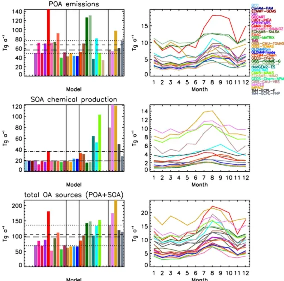
have similar seasonality in POA emissions that are driven by tPOA, with increased emissions during Northern Hemisphere summer due to the enhanced contribution of Northern Hemi-sphere biomass burning emissions from temperate and boreal forests to the total POA fluxes. In addition, several models include SOA sources in tPOA as explained earlier, scaled by BVOC emissions, which also peak during Northern Hemi-sphere summer (Guenther et al., 1995, 2006); this contributes to a seasonal cycle of tPOA that is caused by the trSOA treat-ment as part of tPOA, and should not be interpreted as a tPOA seasonality. Also note that contrary to biomass burning, an-thropogenic tPOA sources have no seasonality in their emis-sion inventories. The IMPACT model appears to have the opposite seasonality, with maximum POA emissions during winter and minimum from late spring to early summer, due to the fossil fuel emissions scaling to fit observations (Wang et al., 2009). The minimum of the emissions for all mod-els except IMPACT is during Northern Hemisphere spring, when neither biomass burning nor the photochemical trSOA sources (included in tPOA by many models) are high.
The POA emissions variability from phase II is roughly the same as that of the OA variability from ExpA, which indicates that the significant uncertainties in the POA emis-sions in global models since AeroCom phase I have not been reduced. However, some models have very high POA emissions, due to the recently developed parameterizations of mPOA sources in global models. These highly uncertain sources were absent in AeroCom phase I.
4.1.2 Chemical production
The chemical production of SOA is much more complex compared to the POA emissions. Firstly, many models in-clude SOA sources as primary emissions, which are inin-cluded in tPOA (see Sect. 1.8 and Table 1). This type of source was used during AeroCom phase I experiments (Dentener et al., 2006). The direct consequence of this assumption is that any uncertainties resulting from the OA sources in ExpA are only related to the POA emissions, since the SOA sources were identical across models. For AeroCom phase II, 13 out of 31 models still use this source parameterization (Ta-ble 2), while 5 models use a simple SOA production rate based on gas-phase oxidation, which then forms non-volatile SOA. These 18 models have a median SOA source strength of 19.1 Tg a−1(mean 20 Tg a−1)and a standard deviation of
4.9 Tg a−1(Fig. 2). Very few models that include this source
have provided budget information on the seasonal variabil-ity of its SOA source, since it is implicitly included in the tPOA sources and is not tracked separately. However, it has a virtually identical seasonality to that of the monoterpene emissions adopted in each model.
From the other models that include a more complex cal-culation of SOA chemical production, there is a large inter-model variability in the source flux, with median 51 Tg a−1
(mean 59 Tg a−1)and 38 Tg a−1 standard deviation, based
K. Tsigaridis et al.: The AeroCom evaluation and intercomparison of organic aerosol 10857
Figure 2.Top row: POA emissions included in models (before POA evaporation in the case of GISS-CMU-VBS); middle row: SOA chemical production (including the pseudo-primary SOA source, where applicable); bottom row: total OA sources (sum of top and middle rows) for the annual mean (left column; short dashes: mean; long dashes: median; dotted lines: 25/75 % of the data) and seasonal variability (right column). Note that not all models have submitted annual budget data, and fewer have submitted seasonal information; thus, their corresponding columns/lines are not shown. The models are grouped based on their complexity, as separated by vertical solid lines in the annual mean budgets. Groups from left to right: SOA is directly emitted as a non-volatile tracer; SOA is chemically formed in the atmosphere, but is considered non-volatile; SOA is semi-volatile; SOA is semi-volatile and also has VBS (GISS-CMU-VBS) or multiphase chemistry sources.
models (IMAGES, IMPACT, GISS-CMU-VBS, HadGEM2-ES, OsloCTM2 and TM4-ECPL-F) include very strong SOA sources of 120, 119, 79, 64, 53 and 49 Tg a−1, respectively,
followed by CCSM4-Chem (33 Tg a−1) and GEOS-Chem (31 Tg a−1). About 42 % (50 Tg a−1)in IMAGES are due to non-traditional sources (glyoxal and methylglyoxal). The tra-ditional SOA source in IMAGES accounts for water uptake, which is found to increase the partitioning of semi-volatile intermediates (Müller, 2009). Monoterpenes alone account for about 40 Tg a−1. This large contribution is due to the
very high SOA yields (∼0.4) in the oxidation of
monoter-penes by OH in low-NOx conditions, which are justified by the formation of low-volatility compounds like hydroxy di-hydroperoxides (Surratt et al., 2010). IMPACT has
sev-eral non-traditional SOA sources from aqueous chemistry, which locally can contribute as much as 80 % of the total OA mass. CAM5-MAM3 and IMPACT also include anthro-pogenic precursors. CAM5-MAM3 also uses a factor of 1.5 SOA yield increase in order to reduce anthropogenic aerosol indirect forcing, by elevating the importance of SOA during the preindustrial period (Liu et al., 2012). As mentioned be-fore, HadGEM2-ES does not calculate SOA production ex-plicitly; instead, it uses the Derwent et al. (2003) climatol-ogy from STOCHEM, which calculates an SOA formation of 64 Tg a−1. For comparison, satellite-constrained studies
esti-mate that the total OA formation (primary and secondary) can be as high as 150 Tg a−1, with 80 % uncertainty (Heald
formation rate between 50 and 380 Tg a−1, with 140 Tg a−1
being the best estimate (Spracklen et al., 2011), while Hal-lquist et al. (2009) estimated, using a top-down approach, that the best estimate for the total biogenic SOA formation is 88 TgC a−1, out of a total 150 TgC a−1of OC.
The case of GISS-CMU-VBS deserves focus. This model calculates SOA production based on the VBS approach. Its secondary source of 79 Tg a−1 includes not only newly
formed SOA both from POA and intermediate-volatility or-ganics, but also gas-phase chemical conversion of organic mass that has evaporated from emitted POA, to produce less volatile organics, i.e., mass that has undergone aging in the atmosphere. The traditional SOA sources from bio-genic VOC are included in this model like in other models that use the two-product model, but also the chemical con-version of intermediate-volatility organics to less volatile OA is taken into account, again with the use of the VBS. Over-all, GISS-CMU-VBS presents a similar seasonal pattern of SOA chemical production as other models, but shifted by one month, i.e., peaking in August, when biomass burning is at its maximum in the Northern Hemisphere, instead of max-imizing in July, when photochemical activity and biogenic VOC emissions are higher globally. This might be due to the inclusion of the intermediate-volatility compounds as SOA precursors, which also have large biomass burning sources. CCSM4-Chem and GEOS-Chem also have a shift in the sea-sonal maximum. For CCSM4-Chem this is due to strong pro-duction from biomass burning sources, while in the case of GEOS-Chem the seasonal cycle seems to be driven by pro-duction from Amazonia, which is related with both biogenic and biomass burning emissions.
The total OA sources during ExpA were very similar to the total sources from the phase II experiments (median 97 Tg a−1 both in ExpA and here), while ExpB had much lower total OA sources, 67 Tg a−1 (Fig. 1). All of these sources include SOA, either as pseudo-emissions (phase I) or from a variety of parameterizations (phase II). The models from phase II present a much higher variability in their total OA sources, which is primarily attributed to the SOA chem-ical production variability that was not present in ExpA. 4.1.3 Burden
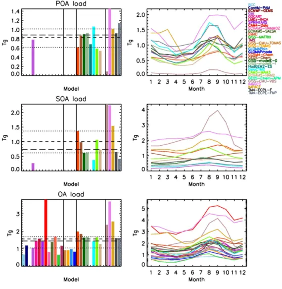
From the models that have submitted POA burden data (also termed load; the mean total mass in the atmosphere), both its seasonality and amplitude largely follow those of the corre-sponding POA emissions (Fig. 3), with two notable differ-ences. The two GISS-modelE models have much lower POA burdens (but similar seasonality) than their emissions would imply. The reason is that the mPOA fraction of POA has a very short lifetime of∼1.5 days, since mPOA is assumed
to be internally mixed with fine-mode sea salt, which is re-moved efficiently due to wet scavenging (Tsigaridis et al., 2013). This keeps the overall load of POA fairly low, and comparable with the models that do not have mPOA. The
other difference is GISS-CMU-VBS, which also has a much lower POA load than their emissions would suggest. This is due to the POA aging parameterization, which converts POA into SOA, drastically reducing the POA burden. The other models appear to have the expected POA load, given their emissions, including IMPACT, whose different seasonal vari-ability of the emissions is also reflected on its OA load.
For the computed SOA load (Fig. 3), all models assume that SOA is very soluble, with 80–100 % of its total mass considered soluble, which results in similar globally aver-aged removal rates across the models. This means that the differences in the SOA loads are expected to be driven pri-marily by the SOA chemical production, similar to how the POA load is driven by emissions. This is indeed the case for almost all models, with GISS-CMU-VBS, IMAGES, IM-PACT, CCSM4-Chem and CAM5-MAM3 having the highest loads, exceeding 1 Tg, with the first two models being as high as 2.3 and 2.2 Tg, respectively, and GEOS-Chem being just below 1 Tg. Spracklen et al. (2011) estimated a global SOA burden of 1.84 Tg, similar to the high-end models that partic-ipate in the current intercomparison, but for a SOA formation rate of 140 Tg a−1, which is about 20 % higher than IMPACT
and IMAGES (the models with the strongest SOA formation here), and about 3 times higher than the median SOA forma-tion rate of the models that have a complex SOA parameter-ization. ECHAM5-HAM2 calculates an increasing load over the course of 1 year, which is related to the short spin-up time of 3 months, which is not sufficient for the upper tropo-spheric SOA to reach equilibrium. GEOS-Chem simulates an inverse seasonality when compared with other models, with the maximum load calculated during Northern Hemi-sphere winter and the minimum during Northern HemiHemi-sphere summer. The cycle seems to be dominated by the SOA load over the Southern Ocean; probably the removal processes are slower than other models there, thus SOA may form a uni-form band between 30 and 50◦S during the whole austral
summer.
K. Tsigaridis et al.: The AeroCom evaluation and intercomparison of organic aerosol 10859
Figure 3.Same as in Fig. 2, for the POA/SOA/OA load.
The total OA load is calculated to be mostly lower than the sulfate load in the models that reported budget values for both aerosol components, with a median value of the OA / SO2−
4 mass load ratio of 0.77 (mean 0.95). The ra-tio lies in the range 0.26–2.0; CAM4-Oslo, CAM5-MAM3, GEOS-Chem, GISS-modelE-G/I, IMAGES, IMPACT, and TM4-ECPL-F/FNP calculate values above 1, which means that annually on the global scale OA dominates over sulfate aerosols. That was the case for 5 out of 16 models during roCom phase I (Textor et al., 2006). Note however that Ae-roCom phase I models were simulating the year 2000, while here we simulate the year 2006; interactive chemistry, new sources (isoprene, mPOA and ntrSOA) and different emis-sion inventories also contribute to significant differences be-tween the two studies. One has to be reminded that even in AeroCom phase II, many models used some emission inven-tories from a year other than 2006 (Tables 4 and 5).
4.1.4 Deposition
Dry deposition is a minor removal pathway for OA, ac-counting for a median of 13 Tg a−1 (range 2–36 Tg a−1)
and a mean of 15 Tg a−1 (standard deviation of 10 Tg a−1;
much smaller in GISS-TOMAS in order to have low enough dry deposition fluxes, which does not appear to be the case.
Other than the two TOMAS models, of the remain-ing models that have submitted dry deposition flux data, three models calculate very low fluxes: ECHAM5-HAM2, ECHAM5-HAMMOZ, and TM5, with the latter already mentioned earlier. The first two models use ECHAM5 as the host model, and all three use the M7 aerosol micro-physics module (Vignati et al., 2004). As for the TOMAS case, this is strong evidence that the M7 module does not al-low OA to deposit as fast as in most other models; SALSA, which uses the same host model as ECHAM5-HAM2 and ECHAM5-HAMMOZ, calculates higher dry de-position fluxes than the two ECHAM5 models with M7. The largest difference in dry deposition between the two aerosol microphysics schemes comes from the treatment of external mixing of OA in the accumulation sized particles. ECHAM5-SALSA includes soluble and insoluble OA in the accumu-lation mode, while HAMMOZ and ECHAM5-HAM2 include only soluble OA. In addition, EMAC, which uses a sectional version of M7 called GMXe, does not calcu-late as low a dry deposition as the models that use the modal version of M7. The fact that there are other models with aerosol microphysics parameterizations in this intercompari-son, both modal and sectional, that do not calculate such low dry deposition fluxes, suggests that it is not a general aerosol microphysics calculation issue.
Comparisons of phase I models results for ExpA and ExpB strengthen this conclusion, since the model with the lowest OA dry deposition flux of ExpA (MPI_HAM; 5 Tg a−1)and
that of ExpB (TM5; 1.7 Tg a−1)both use the aerosol
micro-physics module (M7). This scheme appears to be responsi-ble for the lowest dry deposition fluxes calculated by the models that participate in the present intercomparison: the updated versions of these two phase I models, ECHAM5-HAM2, ECHAM5-HAMMOZ and TM5, participate in the phase II experiment and simulated the lowest dry deposition fluxes among all phase II models, together with the GISS-CMU-TOMAS and GISS-TOMAS models that did not par-ticipate in phase I. Whether the above explanation suffices to explain the low dry deposition, or other processes are in-volved as well, like very strong wet removal that does not allow time to dry deposition to become effective, the cal-culated aerosol size distribution, the aerosol properties that impact dry deposition rates, or something else, remains to be explored by dedicated deposition flux model–data com-parisons. Also note that we have not assessed this feature of the models against observations, so we do not know which models are closer to observations.
CAM4-Oslo has the highest dry deposition flux of 36 Tg a−1, which is due to the high OA load. BCC follows with 33 Tg a−1, which is then followed by the two
GISS-modelE models and IMAGES with∼28 Tg a−1. In the case
of the two GISS-modelE models, this is due to the strong re-moval of mPOA, which is internally mixed with sea salt (as
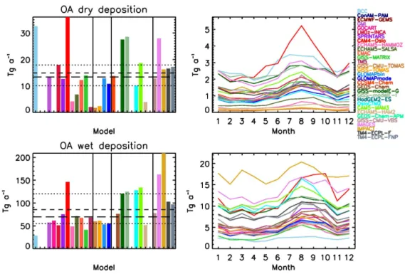
explained earlier), while for IMAGES, it is due to the high OA load, as a result of strong trSOA formation. BCC uses a smaller mass mean diameter than the size distribution of POA emissions, which can explain the high dry deposition flux (Zhang et al., 2012). Despite these large differences be-tween models, the calculated dry deposition fluxes follow the same seasonal pattern as the aerosol load presented earlier (Sect. 4.1.3 and Fig. 4).
The effective dry deposition rate coefficient, defined as the ratio of the dry deposition flux over the aerosol burden that is being deposited (Textor et al., 2006), ranges from 0.005 to 0.13 days−1, with a median value of 0.025 days−1,
a mean value of 0.029 days−1 and a standard deviation
of 0.046 days−1. The diversity (defined as the standard
devi-ation over the mean) has increased since AeroCom phase I, from 0.62 to 0.87. BCC has the largest effective dry deposi-tion rate coefficient, 0.13 days−1, more than double that of
any other model. The models with very low dry deposition fluxes are the ones that have the lowest effective dry deposi-tion rate coefficients, all below 0.014 days−1, supporting the hypothesis that their dry deposition flux is probably too low. By far the most important removal mechanism across all models is wet deposition (Fig. 4). Due to similar OA solubility assumptions across all models, the wet deposi-tion flux largely follows the OA load, both in the annual budget and the seasonality. IMPACT has the highest wet deposition flux of all models (209 Tg a−1), followed by
IMAGES (163 Tg a−1), CAM4-Oslo (146 Tg a−1),
CAM5-MAM3 (134 Tg a−1), OsloCTM2 (128 Tg a−1) and
GISS-modelE-G/I (120/125 Tg a−1, respectively). These are the
models with the highest OA sources (Fig. 2), thus also with the highest sinks. Wet removal of OA is simulated to range from 28 to 209 Tg a−1for the 26 models that reported fluxes,
with mean (median) standard deviation values of 86 (70) 43 Tg a−1, which is on average 85 % of the total OA depo-sition.
The effective wet deposition rate coefficient ranges from 0.09 to 0.24 days−1, with a median value of 0.15 days−1,
a mean value of 0.16 days−1 and a standard deviation of
0.04 days−1. The diversity since AeroCom phase I has
vir-tually not changed, with a slight increase from 0.27 to 0.28. OsloCTM2 has the highest effective wet deposition rate co-efficient, and LMDz-INCA the lowest.
Wet removal, which together with aerosol sources is a ma-jor driver of the calculated aerosol lifetime and load, presents a much higher variability in the phase II models (Fig. 1). This is largely due to the consideration of SOA formation, which is responsible for the large variability in OA sources and bur-den in the models, as well as to differences in the assump-tions on SOA solubility and aging.
4.1.5 Lifetime
K. Tsigaridis et al.: The AeroCom evaluation and intercomparison of organic aerosol 10861
Figure 4.Same as in Fig. 2, for the dry/wet OA deposition.
a species is calculated as the ratio of the species burden over its total removal; in the case of aerosols, the removal is dry and wet deposition. Unfortunately, while most model groups have submitted total OA diagnostics to calculate the OA life-time, few have submitted the diagnostics required to calcu-late the global mean POA and SOA lifetimes.
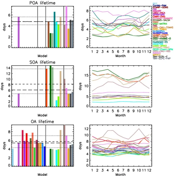
The calculated median POA lifetime from the 13 models that reported relevant data is 4.8 days (mean 4.8±1.4 days).
The modeled lifetime ranges from 2.7 days for the two modelE models to 7.6 days for IMAGES (Fig. 5). The GISS-modelE models have the lowest lifetime, which is consistent with roughly two-thirds of POA being removed rapidly with sea salt (as mPOA). There is no clear seasonal signal on the calculated POA lifetime.
The SOA lifetime calculated by 12 out of 31 models also lacks a clear seasonal signal (Fig. 5). The GISS-modelE-G/I models, CCSM4-Chem, ECHAM5-HAM2 and GISS-CMU-VBS have the highest SOA lifetime of 15/14, 14, 13 and 10 days, respectively, which is related to large amounts of SOA in the upper troposphere, where there is virtually no re-moval mechanism and therefore SOA lifetime is enhanced, until atmospheric circulation or sedimentation brings it to lower layers where it becomes susceptible to removal. For the remaining models that provide information, the calcu-lated SOA lifetime ranges from 2.4 to 6.8 days. The median SOA lifetime from all models that provide budget informa-tion is calculated to be 6.1 days (range 2.4–14.8 days), higher than the median POA lifetime. Anthropogenic POA, which in general is more hydrophobic than SOA, is almost exclu-sively emitted close to surface and below clouds, making
it more susceptible to dry and wet removal; biomass burn-ing POA can be emitted at higher altitudes (Dentener et al., 2006), while a significant amount of SOA is formed above clouds in the models, where temperatures are low. For in-stance, in TM4-ECPL-FNP, about 42 % of the total SOA mass is formed in the free troposphere, while 98 % of POA mass is emitted in the boundary layer. Furthermore, although one might expect that SOA is more soluble, thus more sus-ceptible to removal, this does not appear to be reflected in the model results; the reason is that SOA can be formed above clouds and avoid removal for long periods of time.
Twenty-four models provide sufficient information to cal-culate the total OA lifetime, which lies in the range of 3.8–9.6 days, with a median of 5.4 days and a mean of 5.7±1.6 days (Fig. 5). GISS-CMU-TOMAS has a very
strong seasonality in the calculated OA lifetime, with a max-imum during late Northern Hemisphere spring and a mini-mum during late Northern Hemisphere fall, and GISS-CMU-VBS has the highest OA lifetime of all the models. As in the case of POA and SOA, there is no clear seasonality in the OA lifetime across models.
Figure 5.Same as in Fig. 2, for the POA/SOA/OA lifetime.
believed to be significantly underestimated in global models (Spracklen et al., 2011), as also supported by observations that indicate large amounts of processed OA in the atmo-sphere (Jimenez et al., 2009).
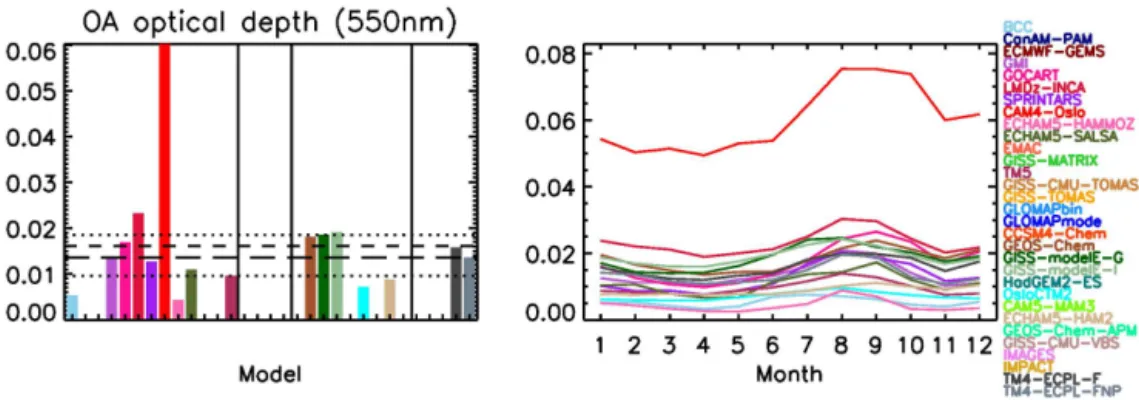
4.1.6 Optical depth
The aerosol–cloud interactions that comprise the indirect ef-fect have been studied with many of the models used here (e.g., Quaas et al., 2009), and the direct effect has been stud-ied previously, both during AeroCom phase I (Kinne et al., 2006; Schulz et al., 2006) and phase II (Myhre et al., 2013; Samset et al., 2013). The impact of the direct and indirect effects of organic aerosols on climate is beyond the scope of the present study. Still, for completeness, we performed a comparison of the OA optical depth at 550 nm (Fig. 6). It has to be noted that this is not always straightforward, or even possible: models that include aerosol microphysics or internally mixed aerosols cannot always separate the aerosol optical depth (AOD) of the organic component of the aerosol