Ficha catalográfica elaborada pela Biblioteca Mario Henrique Simonsen/FGV
Golfín, Felipe Flores
Exclusivity contracts and competition: the case of the Brazilian fuels market, 2016 / Felipe Flores Golfín. – 2016.
30 f.
Dissertação (mestrado) Fundação Getulio Vargas, Escola de Pós Graduação em Economia.
Orientador: André Garcia de Oliveira Trindade. Inclui bibliografia.
1. Combustíveis Brasil. 2. Contratos de exclusividade. 3. Concorrência. I. Trindade, André Garcia de Oliveira. II. Fundação Getulio Vargas. Escola
de PósGraduação em Economia. III. Título.
Abstract
Exclusivity contracts can help stations by providing brand-value that allows them to obtain higher profits, relative to unbranded retailers. However, branded retailers may have a stronger negative effect over its competitors’ profits. It is not clear which one of these two effects dominates (brand-value vs competition effect). Therefore, the impact of exclusivity over the number of participants in the downstream mar-ket is not determined. In this paper, I empirically study the effects of exclusivity agreements on competition in the Brazilian gasoline sector. In order to do so, I estimate an entry model of endogenous product-type choices using data of retailers’ locations and contract choices along with data from the 2010 Brazilian Census. I use my estimates to simulate entry decisions under two counterfactual scenarios: i) mandatory exclusivity and ii) no exclusivity.
KEYWORDS:vertical relations, exclusive contracting, vertical constraints, gasoline markets
Contents
1 Introduction 6
2 Related Literature 8
2.1 Theoretical Literature on Exclusivity Agreements . . . 8
2.2 Empirical Literature on Exclusivity Agreements . . . 9
2.3 Empirical Literature on Two-Period Entry Models . . . 9
2.4 Empirical Literature on Gasoline Markets . . . 10
2.5 Relation to this work . . . 11
3 The Brazilian Fuels Market 12 4 Theoretical Framework 14 5 Data 16 5.1 General Description . . . 16
5.2 Reduced Form Evidence . . . 18
6 Estimation Strategy 20 7 Results 21 7.1 Probit Analysis . . . 21
7.2 Structural Model . . . 21
8 Counterfactual Exercise 24
List of Figures
1 Gasoline Production and Distribution Chain . . . 12
2 Potential locations - S˜ao Jose do Rio Preto, SP . . . 16
3 Dispersion of stations by type . . . 19
4 Population-Probability elasticity . . . 23
5 Income-Probability elasticity . . . 23
6 Counterfactual Results . . . 24
List of Tables
1 Distribution of brands among retailers. . . 132 Demographic Summary Statistics . . . 17
3 Industry Summary Statistics . . . 18
4 Number of Retailers vs Demand Proxies . . . 18
5 Competition effect by type . . . 19
6 Exclusivity decision: Probit Analysis . . . 21
7 Estimation Results . . . 22
8 Markets used in the estimation. . . 29
9 Continuation: Markets used in the estimation. . . 30
1
Introduction
Exclusive dealing (ED) is a practice in which a retailer agrees to sell the products of only one distributor. This type of agreement is prevalent in many sectors, such as insurance, car dealers or gasoline markets. The practice has been labeled as anticompetitive in the past1, however there is no conclusive opinion over its effects on competition in the
downstream market. Exclusive dealing can generate increases in the wholesale prices by limiting competition in the upstream market, it also can mitigate any double marginal-ization problem or improve the quality of the final product. Neither one of these two alternatives has a clear effect over the number of participants in the downstream market.
I explore the effect of exclusive arrangements on entry in the brazilian gasoline market. In Brazil, companies cannot directly participate in both the distribution and retailing of gasoline. Therefore, a common agreement in this industry is one in which a gasoline station signs an exclusivity contract with its provider.
Gasoline markets is an appropiate scenario to study this topic, not only because of the structure of contracts, but also because it is a relevant market in most countries. In the United States, for example, consumers devote 2.25% of their annual income on gasoline purchases and in Brazil a gallon of fuel represents almost 20% of an average consumer’s daily income (Bloomberg (2014)).
To measure the effect of exclusive dealing on competition I construct a static model of firm entry based on (Mazzeo, 2002) andSeim (2006). In the model, each market con-sists of a set of locations. Potential entrants choose a location and a type (exclusive or independent) to enter the market, and they do so simultaneously. Firms have private information; therefore, they maximize the expected profit across locations in order to make entry decisions. I estimate the model with data from the Brazilian fuels market.
The model is estimated using data from two different sources. From the ANP - Agencia Nacional de Petroleo2 I obtained a database with the addresses of all the retailers that
were active in 2010, from the IBGE - Instituto Brasileiro de Geografia e Estat´ıstica3 I
obtained information on the limits of each census tract, which I used to define the poten-tial locations within each market. In addition, I use data from the 2010 Brazilian Census to calculate some demand proxies (population, mean family income, education, among others) for each census tract.
1
Two well-known cases in the U.S. are Standard Fashion v. Magrane and Houston Tampa Electric v. Nashville Coal where a court determined that exclusivity contracts attempted against competition.
2
ANP: Regulatory body of the Brazilian gasoline sector. 3
After estimating the benchmark, I simulate the expected number of participants in the market under two counterfactual scenarios: i) firms can only enter as exclusive retailers and ii) absence of exclusive contracts.
First, I find that demand proxies, such as population and income, positively affect the profits of branded and unbranded retailers. In addition, I conclude that the effect of these variables is stronger for exclusive stations. For example, an increase in the population of a particular location can raise the probability of entry of an exclusive retailer by 17% more than it would that of an independent one.
Second, the model’s estimation suggests that the presence of an extra branded retailer in the market has a negative effect over profits. However, the presence of an additional independent retailer only has a negative effect on profits when it is located within a 1km radius of the firm.
The counterfactual results indicate that exclusivity contracts have a negative effect over the expected number of retailers in the markets. The results suggest that a ban on ex-clusivity agreements could increase the number of stations, on average, by 50%.
2
Related Literature
This paper relates to three different literatures, the one studying the effects of exclusiv-ity contracts on competition and welfare, the literature on endogenous entry and more specifically the literature on gasoline markets. In this section I will discuss the main papers of each one of those literatures and their relation to my work.
2.1
Theoretical Literature on Exclusivity Agreements
The study of exclusive dealing began with a series of theoretical papers analyzing the case of an industry were the seller signs exclusivity agreements with the final consumer. The seminal paper of the area by Rasmusen et al. (1991), argues that exclusive dealing has the potential to be an anticompetitive practice. It presents an environment where firms need to serve a minimum number of consumer to enter the market. In this case, the incumbent may sign exclusive agreements with enough buyers to impede entry of any competitor.
Bernheim and Whinston (1998) and Segal and Whinston (2000) build on this paper and study a similar framework; however, they allow for a richer model and show that exclusivity agreements can generate exclusionary and non-exclusionary equilibria. Fu-magalli and Motta(2006) study the case of a vertically integrated industry in which the manufacturers sign exclusivity contracts with the retailers, the authors prove that the possible foreclosing effects of exclusivity clauses depend on the intensity of competition in the downstream market.
Chen and Riordan (2007) show that the interaction between vertical integration and exclusive dealing can generate a foreclosure effect that neither one of the two types of contracts can produce on its own. They present a framework in which a vertically inte-grated firm forces independent downstream retailers to sign exclusive agreements, this in turn drives upstream competitors out of the market. Other papers have departed from the discussion of the foreclosure effect and focused on different potential consequences of exclusive agreements. de Meza and Selvaggi (2007) presents a model in which ED can help foster relation-specific investments.
One of the most recent contributions to the theoretical literature is the paper byJohnson
(2015). The author drops one of the main assumptions of the previous literature and uses a framework in which no supplier has an inherent contracting advantage over another. In his model, partial exclusivity4 may arise and exclusivity may be beneficial to upstream
4
and downstream firms by raising final prices. This paper is of particular interest to my study because it discusses the effects of the exclusive arrangements on the downstream market, which so far had not been explored in the literature.
2.2
Empirical Literature on Exclusivity Agreements
As seen above the theoretical literature on ED is extensive and shows that exclusivity contracts can have ambiguous effects on competition and welfare. Yet, the empirical re-search is very scarce and similarly to the theoretical work the results are not conclusive. For example, Asker (2005) finds no evidence for foreclosure effects of exclusivity in the Chicago beer markets. On the other hand, Lee (2013) estimates a structural model of the video game industry and concludes that exclusive dealing leads to more competition, but consumers’ welfare would be higher without exclusive relations.
Recently, a few papers have emerged that attempt to close the existing empirical gap.
Soares (2015) estimates a structural model of the Brazilian gasoline market and finds that mergers in the upstream market increase prices and that the network of exclusive retailers affects the size of the increase. Sinkinson(2015) studies the smartphones indus-try in the United States and shows that exclusivity contracts between handset providers and wireless carriers increased prices, but incentivized entry in the market. Nurski and Verboven (2015) asks if exclusive dealing in the European car market creates an entry barrier to downstream firms. The authors use a structural approach to conduct policy counterfactuals and conclude that a ban on exclusive dealing would increase the presence of small dealers.
2.3
Empirical Literature on Two-Period Entry Models
The theoretical model and empirical strategy used in this paper builds on the endogenous entry literature. The seminal papers in this area are Bresnahan and Reiss (1991) and
Bresnahan and Reiss (1990), in these papers the authors consider the entry decisions of homogenous firms and build a two-stage entry game, they then estimate their model with data on the number of participants and demand proxies for a sample of markets in the United States.
competition effect varies by type of firm, however, his model is limited to the extent that the number of types must be small for the model’s estimation to be computational feasible.
Seim (2006) proposes a different approach to model endogenous product type choices, she introduces private information in the firms’ profits, which allows dealing with the computational burden of estimating a model with several product types. The author studies the video retailing industry and builds a model in which firms choose among a set of locations within the market to differentiate from each other. Her model allows for several different types (in the form of locations) and uses demographic characteristic and competition effects to explain firms’ spatial positioning choices.
Orhun (2013) also focuses on an industry with spatial differentiation; the author studies entry choices by supermarkets in the United States. She introduces location specific un-observables into a private information framework similar to the one developed by Seim
(2006).
Cilberto and Tamer (2009) provides a different solution to the problem of multiple equi-libria present in all of the previous models, instead of imposing assumptions on entry decisions the authors use a partial identification approach.
2.4
Empirical Literature on Gasoline Markets
Finally, this paper relates to the literature on gasoline markets. One the most influen-tial papers in this area is Hastings (2004), in this study the author exploits exogenous variation in the number of integrated retailers in the American fuels market to measure the impact of vertical integration on prices and concludes that a larger presence of ver-tically integrated stations increases final prices. In a similar paper Hastings and Gilbert
(2005) examines empirically the relationship between vertical integration and wholesale gasoline prices. They find evidence that vertical integration can increase wholesale prices.
Several authors have focused on aspects of the fuels industry, other than vertical re-lations. Houde et al. (2010) presents a comprehensive survey of the main questions that have been studied in this literature.
2.5
Relation to this work
As seen above, the theoretical literature has suggested that exclusivity agreements have the potential to affect competition in the downstream market. This paper relates to this literature in that it quantifies this effect on a particular industry, by exploring the impact of exclusive contracts on the number of downstream market participants.
The methodology used in this paper follows previous approaches of the two period entry models literature. Specifically, it resembles Mazzeo (2002) in that firms endogenously choose their type. In addition, it follows Seim (2006) by assuming that retailers hold private information about their profit and differentiate from competitors by spreading across locations in within the market.
3
The Brazilian Fuels Market
The current institutional makeup of the Brazilian fuels market was established in the early 2000s by the introduction of the Lei do Petr´oleo. Before the passing of this law the industry was a monopoly in all of its stages (production, refinery and distribution), with the exception of the downstream market. The new law ended the government’s control over final prices and allowed private companies to get involved in every comercial activity of the industry.
The distribution chain of fuels starts with the extraction (or importation) of petroleum which is then processed by the country’s refineries. This stage is heavily dominated by Petrobras-BR (a Brazilian state-owned oil company), that refines almost all of the oil that is consumed in the country. For example, in the period from 2000 to 2007 Petrobras was responsible for 98.7% of the refineries’ production (Ayres and de Freitas (2008)). Among other products, refineries produce Gasoline A that they sell to distributors.
Figure 1: Gasoline Production and Distribution Chain
Source: Petrobras (2015)
Gasoline A in order to produce Gasoline C5. Distributors sell Gasoline C and hydrated
Ethanol to gas stations6.
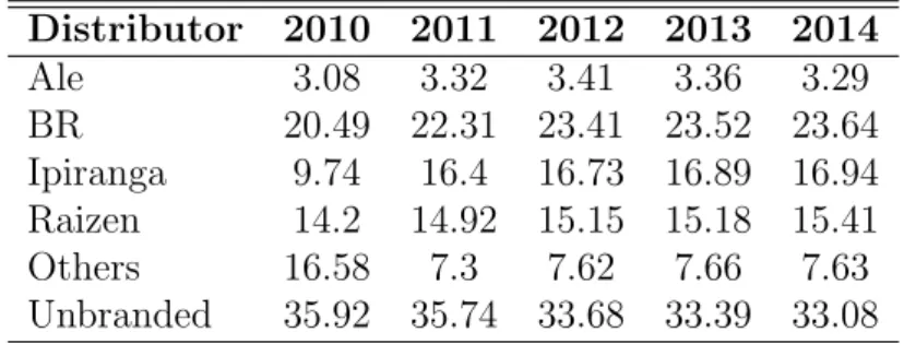
At the final stage of the distribution chain there are the gas stations, which freely set retail prices. By law, distributors cannot operate stations. However, a common practice in Brazil is for a distributor to sign an exclusivity agreement with the gas station that buys its product. This type of contract allows the ”branded” station to utilize the name of the distributor to promote its products (usually the distributor covers the advertising costs), and in turn the station agrees to buy a certain amount of fuels from the distributor at a price set by the latter (de Oliveira and Maia (2012)).
Table 1: Distribution of brands among retailers.
Distributor 2010 2011 2012 2013 2014
Ale 3.08 3.32 3.41 3.36 3.29
BR 20.49 22.31 23.41 23.52 23.64
Ipiranga 9.74 16.4 16.73 16.89 16.94
Raizen 14.2 14.92 15.15 15.18 15.41
Others 16.58 7.3 7.62 7.66 7.63
Unbranded 35.92 35.74 33.68 33.39 33.08
Even though there are several distributors operating in the market, almost 90% of the branded stations have signed exclusive agreements with one of four companies. In table1
I present the market’s brand distribution. As can be seen, Ale, BR, Ipiranga and Raizen dominate the upstream market, approximately 60% of the retailers are associated with one of those four brands. This market composition has remained stable in the past four years, with the exception of Ipiranga’s expansion in 2011. This is one of the interesting facts of the industry, unbranded and branded stations coexist, and unbranded stations hold an important share of the downstream market.
5
The Agency of Petroleum, Gas and Biofuels (ANP) requires that gasoline sold at gas stations must contain 25% of ethanol.
6
4
Theoretical Framework
I follow Seim (2006) and consider a two-period game of entry. In the first stage of the game, a set Fm of retailers decide, simultaneously, whether to enter the market m. Mar-kets are composed by a fixed set of locations, and firms may operate as exclusive or independent retailers.
Each firm that decides to enter must choose a location and a type (independent or exclu-sive) to do so. Let cindex an specific location and type combination. Then, a retailer r
that operates in location-type combination c, receives the following profit in the second period.
πr,c =Dmc β+
X
k
γc,kmnmk +ξm+ǫmr,c. (1)
Where, Dm
c is a vector of demand proxies,nmc refers to the number of firms operating in location-type combination c, ξm is a market level shock and ǫm
r,c is a location-type-firm specific shock. β is a vector of parameters for the demand characteristics andγc,km reflects the competition effect of retailers of different location-type combinations.
A firm that decides not to participate in the market receives the following profit.
πr,0 =ǫmr,0. (2)
I assume that all competitors of a certain type, that are located within a certain distance band of firmr, have the same effect over this firm’s profit. Formally, I make the following assumption about the competition effect within the market.
Assumption 1. Let c, k, k′ index location-type combinations. Then, γm
c,k = γc,km′ = γt,b
if k and k′ are of type t and D
b ≤ dc,k, dc,k′ ≤ Db+1, where Db defines the cutoff of a
particular distance band and dc,k is the distance of location k to c.
This assumption also implies that the effect of exclusive and independent competitors over profits is the same for independent and exclusive firms. In addition, I assume that retailers only observe their own location-type specific shocks.
Assumption 2. Retailer’sr location-type shocksǫmr,1, ..., ǫmr,C are private information and are i.i.d. with extreme-value type 1 distribution.
period. That is, it chooses an optimal location-type combination c∗ such that
E[πr,c∗]≥E[πr,c],∀c6=c∗
E[πr,c∗] +ǫr,c∗ ≥E[πr,c] +ǫr,c,∀c6=c∗.
(3)
Then, the probability of retailer r choosing location-type combination cis given by
pr,c = P(E[πr,c∗] +ǫr,c∗ ≥E[πr,c] +ǫr,c,∀c′ 6=c) (4)
pr,c =
exp(Dcβ+PtPbγt,bE[Nt,bc ])
P
kexp(Dkβ+
P
t
P
bγt,bE[Nt,bk])
.
WhereE[Nc
t,b] is the expected number of competitors of typetwithin a distance band bof locationc. The last equality follows from assumption2. Given that the entry decision of all firms is symmetric, the probability of entry in a particular location-type combination is the same for all retailers. That is, pr,c = p∗c,∀r. Then, for location-type combination
c, the expected number of competitors of a particular type and distance band is equal to
E[Nt,bc ] = (E −1)X c′
Ic,ct,b′p∗c′ (5)
where,E is the expected number of market participants andIc,ct,b′ is equal to one if location-type combinationc′ is of typetand within distance bandbofc, and zero otherwise. Given this, the vector of probabilities forms the following system of equations
p∗ c =
exp(Dcβ+ (E −1)
P
t
P
bγt,b
P
c′I c,c′ t,bp∗c′)
P
kexp(Dkβ+ (E −1)
P
t
P
bγt,b
P
c′I k,c′ t,b p∗c′)
,∀c. (6)
To compute the expected number of firms in the market E, a retailer considers the following probability of entry
pEntry =
exp(ξ)[Pkexp(Dkβ+ (E −1)
P
t
P
bγt,b
P
c′I k,c′ t,b p∗c′)]
1 + exp(ξ)[Pkexp(Dkβ+ (E −1)
P
t
P
bγt,b
P
c′I k,c′ t,b p∗c′)]
. (7)
Considering this expression the firm can compute the expected number of market partic-ipants.
E =F ∗pEntry (8)
5
Data
5.1
General Description
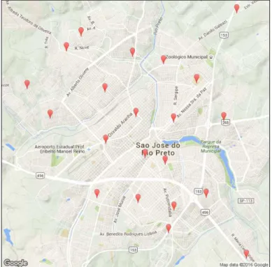
As seen in the model presented above, firms choose whether to enter, their type (exclusive or independent) and a location within the market. In practice, potential locations are the centers of the census tracts7 that belong to the market. To illustrate, in figure 2 I
present the locations for S˜ao Jose do Rio Preto, SP.
The IBGE provides public access to data on the geographic coordinates of the census tracts. However, this information is only available for a selected sample of municipal-ities of each state. Since it is important to have a rich territorial division to allow for the geographical differentiation observed in the fuels retailing industry. The sample was further restricted to include only municipalities with at least six locations (census tracts).
Figure 2: Potential locations - S˜ao Jose do Rio Preto, SP
I then used the Brazilian census to obtain demographic and market characteristics of each census tract. Demographic measures are population, mean income, proportion of people with a car or motorcycle and mean years of education, this data is taken from the 2010 census. In addition, I used the ANP weekly sample of retailers in the fuels industry to obtain the list of active stations in 2010. Then, using information on the retailer’s address, I was able to link each retailer to its respective census tract. With
7
this, I calculated the number of independent and exclusive stations per census tract and linked this to the census data.
Since each market is composed of at least one municipality I excluded municipalities with a population of over 1.5 million. This was done to avoid including groups of re-tailers that do not actually belong to the same market. The final sample consists of 45 markets8, across 18 states with populations ranging between 150 000 and 1 million people.
Table 2: Demographic Summary Statistics
Variable Mean Min. Max.
Market Level (N=44)
Number of tracts 18.80 4 46
Total population 380 307 158 381 932 748
Population of biggest tract 50 531 16 915 185 558
Median population across tracts 25 572 13 507 103 857
Tract Level (N=684)
Years of education 8.10 5.5 10.81
Personal Income 1467.46 194.0 5519.6
Family Income 989.43 117.05 4382.81
Proportion of people with car 0.53 0.01 0.92
Proportion of people with motorcycle 0.24 0.05 0.57
In table2, I present some summary statistics of the markets’ demographic measures. Mar-kets in the sample have, on average, 19 different locations and a population of 380,307 people. The mean proportion of people who own a car across markets is equal to 53% and the tracts median population is close to 25 000 people.
Table 3 provides a summary of the gasoline retailing industry. On average there are 74 retailers per market, however, since the size of the market varies a lot in the sample the number of stations can be as high as 194. Competition is intense among retailers, on average, a station faces five competitors within a 1 km radius and the mean distance to the closest competing location is less than 3 km.
8
Table 3: Industry Summary Statistics
Variable Quantity Proportion
Overall
Number of retailers 3274 100%
Number of branded retailers 2142 65%
Number of unbranded retailers 1132 35%
Variable Mean Min. Max.
Market Level (N=44)
Number of retailers 74.41 27 194
Number of branded retailers 48.68 7 147
Number of independent retailers 25.73 1 63
Tract Level (N=684)
Total number of retailers 4.81 0 81
Closest location in km 2.66 0.19 73.78
Number of stations < 1km 5.88 0 81
Number of stations < 3km 24.48 0 101
Number of stations < 10km 71.75 0 162
5.2
Reduced Form Evidence
In this subsection I present some reduce form results about the retailers’ location and type choices. An important aspect to analyze is how much demographic variables affect the retailers’ location choices, to this purpose I present the results of a simple regression of the number of retailers on population (the unit is 10 000 people) and income (in thousands of reales), controlling for market fixed effects. The results indicate a positive relation between the demand proxies and the number of retailers, as expected. However, these variables appear to explain very little of the location choices. An extra 10 000 people in the census tract, that is approximately half of the mean median population across tracts, is associated with an increase of just one station.
Table 4: Number of Retailers vs Demand Proxies
Dependent Variable
Variable Total # # of Unbranded # of Branded
Population 1.441∗∗ 0.624∗∗ 0.817∗∗
Income 3.760∗∗ 1.097∗∗ 2.663∗∗
Significance levels : †: 10% ∗: 5% ∗∗: 1%
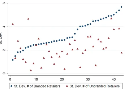
Figure 3: Dispersion of stations by type
To support this claim I plot, for each market, the standard deviation of the number of retailers across locations by type. The circles in figure3represent the standard deviation of the number of branded stations across locations for each market in the data. Each triangle that lies directly below (or above) a circle, represents the standard deviation of the number of unbranded retailers for that same market.
This graphic suggests that independent retailers spread more evenly across the mar-ket, which is consistent with the hypothesis that independent stations shun competition more than exclusive ones.
Finally, it is interesting to analyze if the presence of unbranded and branded competitors has a differentiated effect over location choices. To see this, in table 5 I present the results of a regression of the number of stations (by type) on the number of exclusive and independent competitors within a 1km radius, controlling for market fixed effects and demographic characteristics of the location and of its neighboring census tracts.
Table 5: Competition effect by type
Dependent Variable
Variable Total # # of Unbranded # of Branded
# Branded Competitors <1km -0.417∗∗ -0.165∗∗ -0.251∗∗
# Unbranded Competitors <1km -0.192 -0.095 -0.097
Significance levels : †: 10% ∗ : 5% ∗∗: 1%
ex-clusive competitors within a 1 km radius are associated with one less branded station. Meanwhile four extra independent competitors have no statistically significant effect over the number of branded retailers. This evidence points to differences in how demographic and competition variables affect the location and type choices of firms.
6
Estimation Strategy
To estimate the model presented in section4 with the data described above, I first com-pute the entry probabilities for each location-type combination in the data using equation
6. For each census tractc, I set the center of the tract to be the mean position of all the retailers operating in that location. I then use this center to calculate to which distance band each competing location belongs, that is I compute the dummiesIc,ct,b′,∀c′. Instead of solving the probabilities’ system of equations I exploit the fact that the operator defined by equation 6 is a contraction.
To compute the probabilities I need E, however, the expected number of participants is not observed in the data. I follow Seim(2006) and set E equal to the actual number of firms in the market and to compensate for this I calculate the market level shock ξ that matches the expected number with the observed one. Following equation 8 I can write
ξ = ln(E)−ln(E − F)−ln(X k
exp(Dkβ+ (E −1)
X t X b γt,b X c′
Ik,ct,b′p∗c′)) (9)
This step makes use of the number of potential participants F, I exogenously set this number to be a fixed proportion of the observed number of operating retailers, F =
α∗ E, α >1. Second, I make the following assumption on the distribution of the market
level shock.
Assumption 3. The market level shock ξm is i.i.d. with a normal distribution N(θ, µ).
Given this assumption, I can use the calculated probabilities for each location-type com-bination and the probability of the market level shock to compute the likelihood function of the observed spatial distribution of retailers in each market, for each value of the parameters.
L= Πc [p∗ c(β, γ)]
#Rc
Πmf(ξm|θ, µ) (10)
7
Results
7.1
Probit Analysis
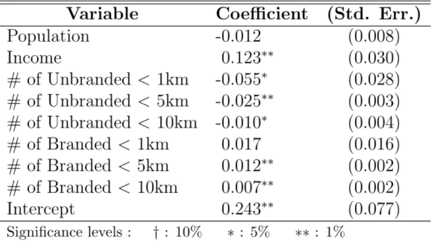
Before presenting the results of the full model I focus on the contract choice at the retailer level. That is, I take as exogenous the retailers’ location choices and study the binary type choice. In table 6, I present the results of a probit analysis of retailers’ exclusivity status. In this specification, I control for demand proxies and potential competition ef-fects.
As can be seen in the table, the presence of more unbranded stations is associated with a lower probability of entering the market as an exclusive retailer. Conversely, more branded stations in any one of the distance bands are associated with a higher probabil-ity of choosing to be exclusive. These results seem to indicate that a simple model is not able to appropriately explain retailers’ contract choices and that the strategic behavior of the stations must be accounted for with a more complex and structural approach, as the one presented below.
Table 6: Exclusivity decision: Probit Analysis
Variable Coefficient (Std. Err.)
Population -0.012 (0.008)
Income 0.123∗∗ (0.030)
# of Unbranded <1km -0.055∗ (0.028)
# of Unbranded <5km -0.025∗∗ (0.003)
# of Unbranded <10km -0.010∗ (0.004)
# of Branded< 1km 0.017 (0.016)
# of Branded< 5km 0.012∗∗ (0.002)
# of Branded< 10km 0.007∗∗ (0.002)
Intercept 0.243∗∗ (0.077)
Significance levels : †: 10% ∗: 5% ∗∗: 1%
7.2
Structural Model
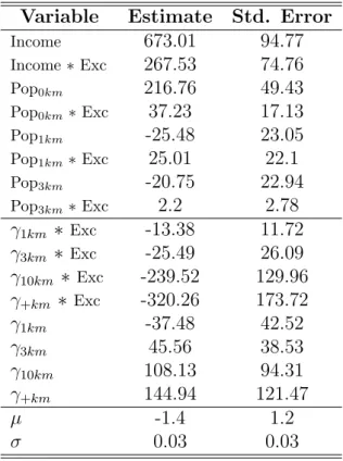
In this section, I present the results of the model’s estimation. As demand proxies, I use population in two different distance bands, and mean personal income at each location. In addition, I consider competition effects in four distinct radii around each location: 1 km, 3km, 10km and more than 10km.
to independent ones. However, a higher population in any one of the two distance bands considered has a negative effect over profit. Even though this is counterintuitive, the effect of population in neighboring locations is small relative to the one of the location’s own population and these coefficients are very unprecise and not significantly different from zero.
Table 7: Estimation Results
Variable Estimate Std. Error Income 673.01 94.77
Income∗ Exc 267.53 74.76
Pop0km 216.76 49.43
Pop0km∗ Exc 37.23 17.13
Pop1km -25.48 23.05
Pop1km∗ Exc 25.01 22.1
Pop3km -20.75 22.94
Pop3km∗ Exc 2.2 2.78
γ1km ∗ Exc -13.38 11.72
γ3km ∗ Exc -25.49 26.09
γ10km ∗ Exc -239.52 129.96
γ+km ∗ Exc -320.26 173.72
γ1km -37.48 42.52
γ3km 45.56 38.53
γ10km 108.13 94.31
γ+km 144.94 121.47
µ -1.4 1.2
σ 0.03 0.03
Income is measured in units of 1000 reais, and it positively affects profits. For exclusive retailers the income coefficient is 40% bigger than that of independent stations. The competition effect varies significantly between branded and unbranded stations. The presence of exclusive competitors in any one of the distance bands has a negative impact on profits. However, for independent stations the competition effect is positive outside of the smaller distance band of 1km. This could be due to the fact that the model cannot fully explain the firms location choices. Therefore, the model associates a higher profit with location that have more retailers.
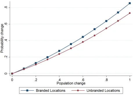
To better illustrate the effect of the demand proxies over entry decisions, I compute the elasticity of the location’s probability to changes in population and income. In figure
4, I plot the mean variation in the location’s entry probability, in response to increases in population.
implies a 20% higher probability of entry; in contrast this same shock over population only increases the probability of entry in independent locations by 17%.
Figure 4: Population-Probability elasticity
Figure 5 presents a similar analysis for income. For exclusive locations, a 70% increase in income translates into a 10% percent increase of the entry probability. An equivalent shock in an independent location increases the entry probability only in 7%. Table 7
also presents the estimated parameters of the market shock distribution. One interesting thing to be noted is that the model predicts a small standard deviation of the market shock.
8
Counterfactual Exercise
In this section, I present the results of the counterfactual simulations. Using the pa-rameters presented in section7, I calculated the expected number of market participants under two different scenarios. First, I considered a case in which firms can only enter as exclusive, but they can still choose the location within the market. Second, I considered an alternative scenario where retailers must be independent.
These two cases are relevant because they allow to understand which one of the two contrasting effects of exclusivity dominates (brand-value vs competition effect). To com-pute the expected number of entrants I used the following equation given by the model
ln(E)−ln(E − F)−ln(X k
exp(Dkβ+ (E −1)
X
b
γt,b
X
c′
Ik,ct,b′p∗c′))−ξ= 0. (11)
Using the data I can recuperate the market’s shock that rationalizes the observed number of market participants, as explained in section 6. Given this market shock I am able to compute the left hand side of the previous expression for each E. Then, the expected number of entrants will be the value of E that solves equation 11.
Figure 6: Counterfactual Results
In figure 6, I plot the expected number of participants for each market under the two distinct scenarios, and the observed number of stations9. For illustrative purposes,
mar-kets are organized from lowest to highest number of stations in the mandatory exclusivity
9
case10. Each square represents the expected number of retailers in the case of mandatory
exclusivity, and each circle directly above a square represents the expected number of re-tailers for that same market in the absence of exclusivity agreements. Triangles represent the actual number of retailers in that market.
The model predicts that under mandatory exclusivity a lower number of stations are expected to enter relative to the case where retailers must be independent. In fact, on average, the expected number of retailers in the independent case is more than double the number under full-exclusivity (116% more). In addition, the model predicts that the actual number of entrants would fall between these two extreme cases for almost every market. Meaning that the absence of exclusivity contracts would increase competition.
The parameters estimates presented in section 7 show two competing effects of exclu-sivity. On one hand, exclusivity allows retailers to extract higher profits from demand proxies. On the other hand, exclusive competitors have a stronger negative effect over profits, relative to independent ones. The counterfactual results suggest that, of the two previous effects, the latter dominates. Intuitively, this is what is driving the higher number of stations in the no-exclusivity case.
10
9
Conclusion
In this paper I explored the effect of exclusivity contracts over competition. I construct an structural model based on the existing two-period entry models literature and estimate it using data from the Brazilian gasoline industry. The results suggest that a retailer’s exclusivity status can have a direct impact over its profits. It is possible that consumers give a positive valuation to the retailer’s brand and that this is justifying the positive coefficient attached to the exclusivity-demand proxies interaction.
The parameters estimates also point out to differences in the effect that independent and exclusive competitors have over profits. The model suggests that the presence of more exclusive stations has a stronger negative impact over profits.
Finally, the counterfactual exercises indicate that exclusivity contracts diminish the ex-pected number of market participants. The model predicts that a prohibition on exclu-sivity contracts would imply an average 50% increase in the number of operating stations.
It is important to note that the two-stage entry models, such as the one developed in this paper, have some limitations. First, the profit functions used in these models do not have a structural interpretation. They lack a pricing and demand function that could explain better what drives the profit of the retailers. Second, these models disregard any dynamic component of the entry decision. In practice, stations can change their type (independent or exclusive) over time and a more complex dynamic model could exploit these decisions to gain information about the retailers’ profit.
A potential avenue for future research is to construct and estimate a more complete model of the industry that allows to better understand the effect that exclusivity has over the retailers’ profits. That is, a model that takes into account aspects such as the consumers’ choice between different stations and the brand choice that stations make. This type of model would help to shed light on the consequences of exclusivity contracts.
References
Asker, J. (2005). Diagnosing foreclosure due to exclusive dealing. Unpublished Manuscript.
Ayres, A. J. S. and T. A. de Freitas (2008). An´alise do mercado de combust´ıveis no brasil e no rio grande do sul. Unpublished Manuscript.
Bernheim, D. and M. D. Whinston (1998). Exclusive dealing. Journal of Political Econ-omy 106(1), 64–102.
Bloomberg (2014). Pain at the pump: Gasoline prices by country. Available at http:
//www.bloomberg.com/visual\discretionary{-}{}{}data/gas-prices.
Bresnahan, T. and P. Reiss (1990). Entry in monopoly markets. Review of Economic Studies 57(3), 833–882.
Bresnahan, T. and P. Reiss (1991). Entry and competition in concentrated. Journal of Political Economy 99(5), 977–1009.
Chen, Y. and M. H. Riordan (2007). Vertical integration, exclusive dealing, and ex post cartelization. The RAND Journal of Economics 38(1), 1–21.
Cilberto, F. and E. Tamer (2009). Market structure and multiple equilibria in airline markets. Econometrica 77(6), 1791–1828.
de Meza, D. and M. Selvaggi (2007). Exclusive contracts foster relationship-specific investment. The RAND Journal of Economics 38(1), 85–97.
de Oliveira, D. P. and V. F. C. Maia (2012). Free competition and exclusivity clause in fuel distribution contracts. Revista de Direito Administrativo 259, 123–147.
Fumagalli, C. and M. Motta (2006). Exclusive dealing and entry, when buyers compete.
The American Economic Review 96(3), 785–795.
Hastings, J. (2004). Vertical relationships and competition in retail gasoline markets: Em-pirical evidence from contract changes in southern california. The American Economic Review 94(1), 317–328.
Hastings, J. and R. Gilbert (2005). Market power, vertical integration and the wholesale price of gasoline. The Journal of Industrial Economics 53(4), 469–492.
Houde, J. (2012). Spatial differentiation and vertical mergers in retail markets for gasoline.
Houde, J.-F. et al. (2010). Gasoline markets.The New Palgrave Dictionary of Economics. Palgrave Macmillan, Basingstoke.
Johnson, J. (2015). Anticompetitive exclusive dealing without exclusion. Unpublished Manuscript.
Lee, R. (2013). Vertical integration and exclusivity in platform and two-sided markets.
American Economic Review 103(7), 2960–3000.
Mazzeo, M. J. (2002). Product choice and oligopoly market structure.The RAND Journal of Economics 33(2), 1–22.
Nurski, L. and F. Verboven (2015). Exclusive dealing as a barrier to entry? evidence from automobiles. Unpublished Manuscript.
Orhun, Y. (2013). Spatial differentiation in the supermaket industry: The role of common information. Quantitative Marketing and Economics 11(1), 3–37.
Petrobras (2015). Cadeia de comercializa¸c˜ao e a composi¸c˜ao dos pre¸cos.
Available at http://www.petrobras.com.br/pt/produtos-e-servicos/
composicao-de-precos/gasolina/.
Rasmusen, E. B., J. M. Ramseyer, and J. John S. Wiley (1991). Naked exclusion. The American Economic Review 81(5), 1137–1145.
Sampaio, R. and L. Sampaio (2013). Competicao entre postos de gasolina em pequenos municipios brasileiros: Uma analise a partir de um modelo de entrada empirico. Econo-mia Aplicada 17(4), 579–598.
Segal, I. R. and M. D. Whinston (2000). Exclusive contracts and protection of invest-ments. The RAND Journal of Economics 31(4), 603–633.
Seim, K. (2006). An empirical model of firm entry with endogenous product-type choices.
The RAND Journal of Economics 37(3), 619–640.
Sinkinson, M. (2015). Pricing and entry incentives with exclusive contracts: Evidence from smartphones. Unpublished Manuscript.
Appendix
Table 8 presents the list of municipalities used in the estimation. It is worth noting that not all markets consist of one unique municipality, for example a single market is composed by Florianopolis, Palhoca and Sao Jose, because of their geographic proximity.
Table 8: Markets used in the estimation.
State Municipality # of tracts # of stations
Alagoas Arapiraca 12 33
Alagoas Maceio 22 144
Amapa Macapa 16 50
Bahia Vitoria Da Conquista 13 37
Bahia Feira De Santana 14 87
Bahia Itabuna 14 33
Bahia Camacari 11 28
Goias Anapolis 10 58
Minas Gerais Divinopolis 7 40
Minas Gerais Governador Valadares 13 44
Minas Gerais Juiz De Fora 14 68
Minas Gerais Montes Claros 21 67
Minas Gerais Sete Lagoas 13 37
Minas Gerais Uberaba 16 75
Minas Gerais Uberlandia 17 115
Mato Grosso Do Sul Campo Grande 8 163
Mato Grosso Do Sul Dourados 9 39
Mato Grosso Rondonopolis 11 55
Para Santarem 10 33
Para Maraba 4 33
Paraiba Campina Grande 20 51
Paraiba Joao Pessoa 10 92
Piaui Teresina 15 123
Parana Cascavel 17 71
Parana Ponta Grossa 15 59
Parana Maringa 19 79
Rio De Janeiro Campos Dos Goytacazes 8 83
Rio Grande Do Norte Mossoro 13 43
Table 9: Continuation: Markets used in the estimation.
State Municipality # of tracts # of stations
Rio Grande Do Sul Caxias Do Sul 26 97
Rio Grande Do Sul Pelotas 19 68
Rio Grande Do Sul Santa Maria 16 46
Santa Catarina Blumenau 19 69
Santa Catarina Florianopolis 46 102
Santa Catarina Sao Jose 46 56
Santa Catarina Palhoca 46 36
Santa Catarina Joinville 29 105
Sao Paulo Bauru 17 98
Sao Paulo Franca 19 86
Sao Paulo Marilia 10 46
Sao Paulo Piracicaba 20 77
Sao Paulo Presidente Prudente 12 65
Sao Paulo Sao Jose Do Rio Preto 22 107
Sao Paulo Sorocaba 20 105
Sao Paulo Votorantim 20 16
Sao Paulo Ribeirao Preto 19 155
Sao Paulo Limeira 6 54
Tocantins Palmas 7 27
Table 10: Counterfactual Results
Expected Number of Entrants
Market No Exclusivity Mandatory Exclusivity Observed Number
1 41.745 16.785 28
2 49 18.997 33
3 48.147 19.707 33
4 49 25.539 33
5 49 25.779 33
6 55 27.95 37
7 65.879 28.507 44
8 59.798 30.364 40
9 40 30.506 27
10 74.947 33.337 50
11 58 35.946 39
12 68.912 36.189 46
13 80.802 38.133 54
14 86.961 38.243 58
15 68.951 38.967 46
16 129 39.198 86
17 102 43.439 68
18 102 43.774 68
19 117 50.173 78
20 138 58.733 92