Significant impact of the East Asia monsoon on ozone seasonal behavior in the boundary layer of Eastern China and the west Pacific region

www.atmos-chem-phys.net/8/7543/2008/ © Author(s) 2008. This work is distributed under the Creative Commons Attribution 3.0 License.

Chemistry

and Physics

Significant impact of the East Asia monsoon on ozone seasonal

behavior in the boundary layer of Eastern China and the west

Pacific region

Y. J. He1,4, I. Uno2, Z. F. Wang3, P. Pochanart4, J. Li3,4, and H. Akimoto4

1_{Earth System Science and Technology, Kyushu University, Fukuoka, Japan} 2_{Research Institute for Applied Mechanics, Kyushu University, Fukuoka, Japan}

3_{LAPC/NZC, Institute of Atmospheric Physics, Chinese Academy of Science, Beijing, China}

4_{Atmospheric Composition Research Program, Frontier Research Center for Global Change, Japan Agency for Marine-Earth} Science and Technology, 3173-25 Showa-machi, Kanazawa-ku, Yokohama 236-0001, Japan

Received: 9 May 2008 – Published in Atmos. Chem. Phys. Discuss.: 5 August 2008 Revised: 27 October 2008 – Accepted: 13 November 2008 – Published: 17 December 2008

Abstract. The impact of the East Asia monsoon on the sea-sonal behavior of O3in the boundary layer of Eastern China and the west Pacific region was analyzed for 2004–2006 by means of full-year nested chemical transport model simula-tions and continuous observational data obtained from three inland mountain sites in central and eastern China and three oceanic sites in the west Pacific region. The basic common features of O3 seasonal behaviors over all the monitoring sites are the pre- and post-monsoon peaks with a summer trough. Such bimodal seasonal patterns of O3are predom-inant over the region with strong summer monsoon pene-tration, and become weaker or even disappear outside the monsoon region. The seasonal/geographical distribution of the pre-defined monsoon index indicated that the East Asia summer monsoon is responsible for the bimodal seasonal O3 pattern, and also partly account for the differences in the O3 seasonal variations between the inland mountain and oceanic sites. Over the inland mountain sites, the O3concentration increased gradually from the beginning of the year, reached a maximum in June, decreased rapidly to the summer valley in July or August, and then peaked in September or October, thereafter decreased gradually again. Over the oceanic sites, O3abundance showed a similar increasing trend beginning in January, but then decreased gradually from the end of March, followed by a wide trough with the minimum in July and Au-gust and a small peak in October or November. A sensitiv-ity analysis performed by setting China-emission to zero re-vealed that the chemically produced O3from China-emission

Correspondence to:Y. He ([email protected])

contributed substantially to the O3 abundance, particularly the pre- and post-monsoon O3peaks, over China mainland. We found that China-emission contributed more than 40% to total boundary layer O3during summertime (60–70% in July) and accounted for about 40 ppb of each peak value over the inland region if without considering the effect of the non-linear chemical productions. In contrast, over the oceanic region in the high monsoon index zone, the contribution of China-emission to total boundary layer O3was always less than 20% (<10 ppb), and less than 10% in summer.

1 Introduction

7544 Y. J. He et al.: Impact of East Asia monsoon on ozone seasonal variations The spring maximum of surface O3was once thought to

be mainly from stratospheric input since the hemispheric circulation in the stratosphere results in the largest strato-spheric O3concentrations during spring in midlatitudes and the stratospheric intrusion strength is found to be strongest in spring (Levy et al., 1985; Staehelin et al., 1994). Some other studies supposed that the high springtime O3 is con-tributed substantially by the accumulation of wintertime an-thropogenically produced O3itself due to the relatively long lifetime of O3 in winter (Liu et al., 1987), or the photo-chemical O3buildup resulting from the wintertime accumu-lation of other precursors such as peroxyacetyl nitrate and hydrocarbons together with the enhancement of solar inten-sity and temperature in spring (Penkett and Brice, 1986; Pen-kett et al., 1993). Wild and Akimoto (2001) and Pochanart et al. (2002) indicated that intercontinental transport con-tributes to the spring maximum in East Asia Pacific rim re-gion. Up to present, the O3spring maximum could be pos-sibly accounted by the combination stratospheric intrusion, intercontinental transport, and regional photochemical pro-duction.

The observed summer minimum of surface O3over East Asia was attributed to the incursion of monsoon which trans-ports oceanic air with less O3to the region and causes lower O3concentration (e.g. Wang, H. X. et al., 2006; Pochanart et al., 2001; Zbinden et al., 2006; Chan et al., 1998; Xu et al., 1997; Luo et al., 2000; Yamaji et al., 2006). Similar phenom-ena have also been observed over other monsoon regions. For example, Pudasainee et al. (2006) found that the observed ground-level O3during the monsoon was lower than the pre-monsoon value in the South Asia pre-monsoon region of India. The East Asia monsoon not only affects the seasonal patters of surface O3 over this region, but also results in the low-est summertime transportation of pollutants over all the year from the Asian continent to Japan and other regions because of the weak Asian outflow and northwestward penetration of the maritime air mass (e.g. Zbinden et al., 2006; Yamaji et al., 2006). Furthermore, Tanimoto et al. (2005) indicated that exchanges between continental and maritime air masses driven by the Asian monsoon play a central role in producing the latitudinal differences in O3seasonality observed at Acid Deposition Monitoring Network in East Asia (EANET) sites. The peak time of spring maximum in the seasonal pattern of O3over East Asia was found to shift by several months at different locations (e.g. Waliguan, Hong Kong, Linan, Qing-dao, Oki, Hedo), from early spring to early summer (e.g. Chan et al., 1998; Luo et al., 2000; Wang et al., 2001, 2006; Yamaji et al., 2006; Li et al., 2007). Transport from the lower stratosphere and intercontinental transport from outside East Asia may partly account for the difference in peak time (Ya-maji et al., 2006). Moreover, besides the common feature of the spring maximum-summer minimum in O3seasonal pat-tern, one peak of summer maximum was also observed at some inland locations of East Asia (e.g. Zhu et al., 2004; Ding et al., 2008). Photochemical activities resulting from

the intense solar radiation and the high regional-scale emis-sion of the O3 precursors, as well as the long-range trans-portation from the polluted regions, were proved to be re-sponsible for the O3 summer maximum (Pochanart et al., 1999; Zhu et al., 2004).

Although a great deal of studies have already given a com-prehensive discussion on the seasonal variations of boundary layer O3, as well as the possible reasons for the peak val-ues, over East Asia, a detailed analysis of the relationship between East Asia monsoon variability and the O3seasonal cycle, with the consideration of geographic dependence, is not presented yet. This study focused mainly on the influ-ence of the summer monsoon on the seasonal cycle and geo-graphic distribution of boundary layer O3over East Asia, by the application of a normalized seasonality monsoon index, based on three years’ observational data from three inland mountain sites in central and eastern China and three oceanic monitoring stations in the west Pacific region. Three full-year nested chemical transport model simulations are also presented. This study is the first to report a detailed com-parison of O3 seasonal patterns between inland the moun-tain sites in central and eastern China and the oceanic sites near Taiwan and southern Japan, on the view of the influence of the East Asia monsoon and the continental anthropogenic emissions.

The structure of this paper is as follows. In Sect. 2, infor-mation about the observational data and the regional chemi-cal transport model is briefly presented; the monsoon index (MI) is also defined. Section 3.1 analyzes in detail the sea-sonal O3patterns at the monitoring sites. Section 3.2 shows the geographical distributions of O3 and MI, and defines a high-MI zone according to the MI spatial distribution. The impact of the East Asia monsoon on the seasonal behavior of O3in the high-MI zone is discussed in Sect. 3.3. A sensitivity experiment is applied in Sect. 3.4 that clarifies the contribu-tions of China-emission to regional O3production. Finally, the main conclusions of this study are given in Sect. 4.

2 Data and methods

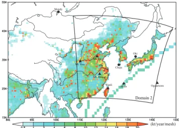
(142.2◦_{E, 27.0}◦_{N) in Japan. The Hedo and Ogasawara sites} were selected from EANET stations (http://www.eanet.cc/ index.html) and are on isolated islands in the southern ocean region of Japan. These two oceanic sites are only slightly af-fected by local and domestic emissions for locating far away from mega-city source regions. In addition, observational data from Mondy (101.0◦E, 51.67◦N), one EANET station, was also used as a typical Northern Hemisphere continental background site. The locations of all of the monitoring sites are shown in Fig. 1. According to the potential impact of con-tinental emission and the East Asia monsoon, all the moni-toring sites are classified into five categories: clean monsoon oceanic site (CMO), polluted monsoon oceanic site (PMO), polluted monsoon inland site (PMI), polluted inland site (PI), and non-monsoon inland site (NMI). Among the monitoring sites, Hedo and Ogasawara are treated as CMO for it’s far away from the continental region and has the least impact of continental emissions, and is strongly affected by the mon-soon; Wanli is classified into PMO, which is located in the strong monsoon region and can be potentially affected by local anthropogenic emissions; Mt. Tai and Mt. Huang are located in the polluted continental region and are impacted strongly by the monsoon, classified into PMI; Mt. Hua is treated as PI, as it’s also strongly affected by regional an-thropogenic emissions and have relatively slight influence of the monsoon; Mondy is located at high latitude region and far away from monsoon influence, and treated as NMI. The O3seasonal patterns at each category site are slightly differ-ent to that at other site in details. Observational data (daily mean values) of three years (2004–2006) from all these sites were systematically analyzed. The missing data due to the equipment malfunction or electronic power-shortage, as well as the data of the intercalary day, are excluded from the anal-ysis.

A three-dimensional nested regional-scale chemical trans-port model, Models-3/Community Multiscale Air Quality (CMAQ, ver 4.4, Byun and Ching, 1999) modeling system released by the US Environmental Protection Agency, was used. Briefly, the model is driven by meteorological fields, which are generated by the Regional Atmospheric Model-ing System (RAMS) with initial and boundary conditions defined by US National Centers for Environmental Predic-tion (NCEP) reanalysis data. The resoluPredic-tion of the model are 80 km and 20 km for the mother domain and the nested domain respectively in horizontal direction, and 19 layers in the sigama-z coordination system up to 23 km. The Regional Emission Inventory in Asia (REAS; Ohara et al., 2007), which is based on several energy statistics, emission factors, and other socioeconomic information and covers the years 1980–2003, was used to drive the model. In this study, three full-year nested simulations were performed for 2004–2006, with the fixed emission inventory of 2003 (shown in Fig. 1) used for the control experiment (referred to as CNTL). The initial fields and monthly averaged lateral boundary condi-tions for most chemical tracers were obtained from a global

Mt. Hua Mt. Tai

Mt. Huang

Wanli _Hedo Ogasawara Cheju

Oki Mondy

(kt/year/mesh) Domain 2

Fig. 1. Geographical distribution of REAS anthropogenic NOx emission intensity (kt/year per mesh) (0.5◦×0.5◦) in 2003, used in the model simulations. The region of the nested CMAQ domain is enclosed by the black square. The locations of monitoring sites are indicated by solid triangles and circles.

chemical transport model (CHASER; Sudo et al., 2002). These monthly lateral boundary conditions were used for all simulations with the assumption of no interannual vari-ation. Additionally, a sensitivity experiment in which China-emission (excluding Taiwan) was set to zero (referred to as COFF) was also conducted to examine the contribution of China-emission to O3abundance over East Asia.

7546 Y. J. He et al.: Impact of East Asia monsoon on ozone seasonal variations

27

Figure 2

(He et al.)

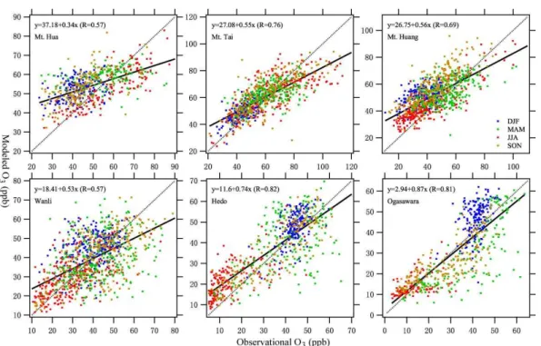
Fig. 2.Comparison of daily mean O3concentration between observations and model simulations during 2004–2006. The blue, green, red, and orange dots represent the correlations between observational and modeled daily mean O₃in winter (DJF), spring (MAM), summer (JJA), and autumn (SON), respectively. The black solid line is the linear regression line of the daily average O3value between the observations and simulations for the period of 2004–2006.

The dynamical normalized seasonality MI is defined as follows:

δ₌ V1₋Vi

V

−2

whereV1andViare the January climatological and monthly wind vectors, respectively, at a given point, and V is the mean of the January and July climatological wind vec-tors at the same point. The norm _kA_k is defined as

kA_{k =} RR S|A|

2_dS1/2, where

Sdenotes the domain of in-tegration (in calculations at a point(i, j ),

Ai,j

≈

√

α

A 2 i−1,j

+

A

2 i,j

+

A

2 i+1,j

cosϕj

+

A

2 i,j₋1

cosϕj−1+ A

2 i,j₊1

cosϕj+1 1/2

,

whereαis the mean radius of the earth andϕj is the latitude at point(i, j )). More detailed descriptions and applications of the dynamical normalized seasonality MI are presented by Li and Zeng (2002, 2003). As the interannual variability of monsoon is not the main topic of this study, for simplic-ity, only three years’ mean wind vectors during 2004–2006 are applied in the calculation instead of the climatological data. This processing method was confirmed to have negli-gible influence on the geographical dependence and seasonal

variation of the MI. Because the computation of the dynam-ical normalized seasonality MI depends completely on wind vectors, the value of MI principally represents the intensity of wind direction alternation from winter to summer. For East Asia, as the northwest wind is predominant in winter, then the higher MI primarily represents the stronger south-east wind in summer. Compared with the orthodox climato-logical monsoon concept, the application of the MI can re-veal the primary features of the special natural phenomenon both its seasonal variation and geographical distribution.

3 Results and discussion

3.1 Validation of simulated O3by comparison with observations

O3value over the oceanic monitoring stations of Hedo and Ogasawara are quite excellent, which was similar to the con-clusions conducted by comparing the CMAQ simulations with the daily O3concentrations at Japanese monitoring sites of EANET during 2002 (Yamaji et al., 2006). In contrast, the three year correlation coefficients are a bit lower at Wanli and the three inland mountain sites. As for Wanli, the poten-tial effect of local emissions (as shown in Fig. 1) should be mainly responsible for the difference between the modeled and observed daily averaged O3 concentrations. With re-gard to the three inland mountain sites, the relatively inferior correlations between the modeled and observed daily mean O3abundance are primarily attributed to the high altitude le-vels. At the top of the mountains, particularly Mt. Hua, the altitude is near or even slightly beyond the boundary layer height. The model simulations are usually hard to capture the sophisticated physical processes at the boundary layer height level exactly in details due to the coarse vertical resolutions (which is set about 500 m thickness near the top of boundary layer height in our model simulations).

As shown in the figures, model simulations slightly over-estimated the lower O3concentrations, and somewhat under-estimated the higher O3values; that reflects that the model simulations may slightly underestimate the O3seasonal vari-ations, as well as the amplitude of the short-term variability. Over the inland mountain sites, model simulations overesti-mated the daily O3magnitude in most days of winter and au-tumn, and underestimated the O3values in most of the higher O3 days of summer and spring. As for the oceanic sites, model simulations overestimated the daily O3concentrations in most days of winter and summer, and underestimated the daily mean O3in most days of spring and autumn. The differ-ent correlations of the simulations and observations between the inland mountain and oceanic sites demonstrated the dif-ferent O3seasonal patterns, which will be detailed discussed in following sections. There are several factors should be responsible for the systematic difference between the model simulations and the observations. Firstly, the application of the emission inventory of 2003 for the simulations of 2004– 2006, as well as the potential underestimation in emission inventory, will lead to the underestimation for the higher O3 concentrations. Secondly, the neglect of the emission sea-sonality in model simulations may slightly underestimate the O3seasonal variations. In addition, the lateral and boundary conditions could result in the small difference between model simulations and observations. The input of the stratospheric O3and the vertical transport may also lead to the overestima-tion or underestimaoverestima-tion for model simulaoverestima-tions, particularly at the inland high mountain sites. Anyhow, despite of the small difference, the model simulations well reproduced the daily O3concentration at all the monitoring sites during the three years, and were qualified for the applications to investigate the O3spatial and temporal distributions over eastern China and west Pacific region.

3.2 Bimodal seasonal patterns of O3

Figure 3a and b show observed and modeled seasonal vari-ations of O3 at the different monitoring sites. All values were calculated based on the daily mean from the three year (2004–2006) average, and then smoothed by 15-day moving average. The most remarkable feature of both the observed and modeled seasonal cycles of O3concentration is the bi-modal pattern with a deep summertime trough. However, the depth and width of the summer trough in the O3 sea-sonal pattern was different between the inland mountain sites (Mt. Hua, Mt. Tai, and Mt. Huang) and the oceanic monitor-ing stations (Wanli, Hedo, and Ogasawara).

Over the inland mountain sites, the observed O3 concen-tration increased gradually from∼40 ppb in January to peak values of about 74, 87, and 63 ppb at Mt. Hua, Mt. Tai, and Mt. Huang, respectively, in June. Then, the observed O3 abundance decreased rapidly and reached the valley value of about 39, 46, and 32 ppb at Mt. Hua, Mt. Tai, and Mt. Huang, respectively, in late July or August. Subsequently, the ob-served O3 abundance recovered, reaching a second peak of

∼62 ppb at Mt. Hua in late August to early September, and of ∼73 and ∼55 ppb at Mt. Tai and Mt. Huang, respec-tively, in October. Finally, the O3 concentration gradually decreased to the end of year. In contrast, over the oceanic sites (Fig. 3a), the observed O3 variation trend exhibited a wide trough from the end of March to October or November, whereas during January–March/October–December, the in-creasing/deceasing trend was similar to or nearly coincided with the O3 variation trend over the inland mountain sites. The two endpoints of the wide O3trough can be understood as the splitting and merging points of O3variation trend be-tween the inland mountain sites and oceanic sites, and they are treated as peaks of O3seasonal variations for the oceanic sites.

7548 Y. J. He et al.: Impact of East Asia monsoon on ozone seasonal variations

28

Figure 3 (He et al.)

Fig. 3. Seasonal variations of observed O₃(a), modeled O₃(b), and the scaled monsoon index(c)over inland mountain sites (red lines) and oceanic stations (blue lines) in East Asia during 2004– 2006. Monthly averaged values at Mondy (101◦E, 51.67◦N) are also presented (black lines). All of the daily mean data were calcu-lated based on the mean of three years’ data and then smoothed by using a 15-day running average. In (a), the inset in the lower left corner shows the typical O₃seasonal patterns for inland sites and oceanic sites; P1 and P2 are the first and second peaks, respectively, and V represents the summer minimum; I, II, III, and IV represent the four phases, which are bounded by the two peaks and the sum-mer minimum, of the full-year O3variations. In (b), Mt. Tai∗shows the O3values with China-emission setting to zero (COFF sensitiv-ity experiment); and delta O3is the modeled O3difference between the CNTL and COFF experiments. In (c), the land region is the area within 110–120◦E, 30–38◦N, including the inland mountain sites of Mt. Hua, Mt. Tai, and Mt. Huang; the oceanic region is the area within 121–129◦E, 24–27◦N, including the oceanic sites of Wanli and Hedo; and Mt. Hua, Mt. Tai, Mt. Huang, Wanli, Hedo, and Ogasawara represent a region of 3◦×3◦centered at each moni-toring sites.

sites. While for the overestimations of summer minimum, the possible reason may come from the lateral boundary con-ditions, but the detailed reason is still unknown. Although the model simulations underestimated the amplitude of O3 sea-sonal variations, the typical seasea-sonal pattern of double peaks and summer minimum is still consistent with observations.

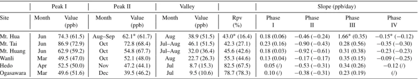
Table 1.Principal parameters of the typical O3seasonal patterns for inland and oceanic sites in East Asia during 2004–2006.

Peak I Peak II Valley Slope (ppb/day)

Site Month Value Month Value Month Value Rpv Phase Phase Phase Phase

(ppb) (ppb) (ppb) (%) I II III IV

Mt. Hua Jun 74.3 (61.5) Aug–Sep 62.1∗(61.7) Aug 38.9 (51.5) 43.0∗(16.4) 0.18 (0.06) −0.46 (−0.24) 1.66∗(0.35) −0.15∗(−0.12) Mt. Tai Jun 86.9 (72.9) Oct 72.8 (68.4) Jul–Aug 46.1 (51.5) 42.3 (27.1) 0.23 (0.16) −0.90 (−0.43) 0.28 (0.56) −0.35 (−0.30) Mt. Huang Jun 62.9 (59.2) Oct 54.8 (67.7) Jul–Aug 32.0 (36.4) 45.6 (42.6) 0.18 (0.03) −0.92 (−0.61) 0.31 (0.38) −0.23 (−0.23) Wanli Mar 49.5 (47.0) Oct 52.1 (48.0) Aug 22.7 (26.3) 55.3 (44.6) 0.13 (0.04) −0.17 (−0.17) 0.35 (0.15) −0.09 (−0.25) Hedo Apr 52.5 (50.0) Nov 47.2 (44.1) Jul 8.7 (15.3) 82.5 (67.5) 0.05 (/) −0.53 (−0.31) 0.34 (0.26) −0.12 (/) Ogasawara Mar 49.6 (51.6) Dec 39.5 (46.2) Jul 9.5 (10.6) 78.7 (78.3) 0.10 (/) −0.38 (−0.31) 0.23 (0.19) (/)

All values are based on three-year mean values and a 15-day running average, the observed data is shown in the upper of each cell, and the modeled value is shown in the lower in the bracket of each cell. The definitions of peak and valley, as well as the four phases, are described in Sect. 3.1, and illustrated in Fig. 2a.RP V=(O3.peak−O3.valley)×100%/O3.peakis the relative amplitude of O3variations between the peak (average of the two peaks) and valley value. The slopes were obtained by linear regression of daily data during each phase, and the less reliable calculated data with the confidence interval larger than 0.05 is omitted, replaced by slash.

∗_{These data are considered much less reliable because of many missing values during the period covered by the phase.}

behaviors. Model simulations shown thatRP V at Mt. Hua (16.4%) was much lower than that at Mt. Tai (27.1%) and Mt. Huang (42.6%), the increase/decrease rates during phase II and III at Mt. Hua were also lower than that at Mt. Tai and Mt. Huang. This phenomenon indicates that the influence of East Asia summer monsoon is relatively weak at Mt. Hua, but much stronger at Mt. Tai and Mt. Huang (detailed dis-cussed in Sects. 3.3 and 3.4). Because a number of missing values were involved in the calculation for observational data at Mt. Hua during phase III and IV, the relevant parameters were less reliable and marked by right superscript star in Ta-ble 1.

The O3seasonal pattern was different at NMI of Mondy, exhibiting only one peak in May. Mondy is a high-latitude site far from the influence of the monsoon (Fig. 4), and the single-peak cycle is the typical O3seasonal pattern over non-monsoon regions of the Northern Hemisphere (Zhu et al., 2004; Ding et al., 2008).

3.3 Seasonal cycle and geographical distribution of O3 in relation to the monsoon index

The distinct O3seasonal patterns at the inland mountain sites and oceanic sites can be partly explained by the differences in the seasonal variations of the MI (Fig. 3c, note that the MI values were converted to a logarithmic scale to show dif-ferences more clearly). Over the ocean region, the MI in-creased rapidly from March and reached a maximum in June and July. In contrast, over the inland sites the MI was much lower than the ocean region during the same period. This dif-ference indicates that the monsoon was much stronger over the ocean than over the land; the south wind, containing the clean maritime air mass, would thus much more intensively affect the oceanic than the inland region. Therefore, begin-ning in April, O3began to decrease over the oceanic sites of Wanli, Hedo, and Ogasawara, but continued to increase over

the inland sites of Mt. Hua, Mt. Tai, and Mt. Huang until the maximum MI appeared in June. Except the remote clean Ogasawara site, the amplitude of MI variations decreased gradually from the polluted oceanic region to deep inland area, with the maximum at Wanli and Hedo and the minimum at Mt. Hua. These geographical distributions of MI varia-tion were consistent with the different O3 seasonal patterns of wide trough at the oceanic sites and narrow trough at the inland, as well as theRP V values of 67%, 45%, 43%, 27%, and 16% at Hedo, Wanli, Mt. Huang, Mt. Tai, and Mt. Hua, respectively. The modeledRP V presented a significant cor-relation with the summer MI values (average of June, July and August):

RP V =0.13+1.04×MIJJA, (R=0.88, P <0.05). Therefore, the application of MI could partly identify the O3 seasonal behavior, particularly the summer trough, over East Asia monsoon region.

7550 Y. J. He et al.: Impact of East Asia monsoon on ozone seasonal variations

29

Figure 4

(He et al.)

Fig. 4.Modeled three-year (2004–2006) mean seasonal distributions of O₃(ppb), wind vectors, and the monsoon index (MI) in the boundary layer (0–1 km) of East Asia for(a)spring (March, April, and May),(b)summer (June, July, and August),(c)autumn (September, October, and November), and(d)winter (December, January, and February). The O3concentration is plotted as red contours, and MI is indicated by colored shading. The high-MI zone is shown by the color shade excluding the southeast region of China. From left to right, the blue triangles are the locations of monitoring sites of Mt. Hua, Mt. Tai, Mt. Huang, Wanli, Hedo, and Ogasawara, all of which are within or adjacent to the high-MI zone.

the strong inflow of the clean maritime air mass. The situa-tion of Wanli is similar with that of Hedo and Ogasawara, so the O3seasonal behavior also presented the “ocean” patterns as Hedo and Ogasawara.

Figure 4 illustrates the modeled seasonal mean geograph-ical distributions of O3, the wind field, and the MI in the boundary layer (0–1 km) over East Asia during the four sea-sons. O3 concentration is plotted as red contour and MI is indicated by colorized shade. The maximal MI in mer demonstrates the strong south/southeast wind of sum-mer monsoon, and the minimal MI in winter manifests the prevailing northwest wind of winter monsoon. In terms of the spatial distribution of the MI during the four seasons, as well as the geographic locations of the monitoring sites, a high MI zone was selected, as shown in Fig. 4 by the colored shade excluding the southeastern China owing to the absence of observations. Generally, the value of MI is higher within this zone than outside of the zone during all seasons.

China, and also moving the high O3center, with maximum values>66 ppb, northward to the area of Beijing. Similar to the distribution pattern in spring, the region with high O3 concentrations extends to northeastern China from Beijing because of the southwest winds. The geographical pattern of the steep latitudinal O3gradient over the monsoon region and the maximum at the northern edge of the monsoon re-gion in spring and summer clearly shows that clean maritime air masses from the Pacific Ocean can carry pollutants north-ward from the polluted industrial regions of southeast China when passing (Tu et al., 2007), and generating regional O3 pollution over the North China region. With the decreasing monsoon strength in autumn, the maximum center of O3 con-centration withdrew from North China and covered most re-gion of eastern China with the value>54 ppb. In winter, the northwest winter monsoon prevails over the region north of 35◦_{N. The band of relatively high O3(>48 ppb) that appears} over the Pacific Ocean region between 25◦_{and 35}◦_{N is from} the long-range transport of pollutants from the continental Asia polluted region (Zhang et al., 2002).

3.4 O3seasonal cycle in the high MI zone

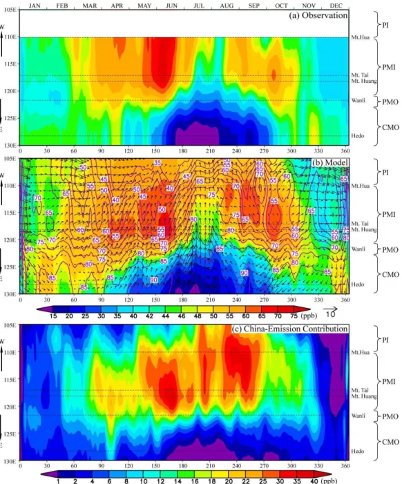
Figure 5a and b illustrate the variations in daily mean O3 (ppb) in the high MI zone shown in Fig. 4 in the observa-tional data and the model simulations, respectively. The ob-served contours were constructed by inverse square distance interpolation of the measurements made at the monitoring sites. Both the observed and modeled data are calculated from three-year means and then smoothed by means of a moving average spanning 4.5◦in longitude over 15 days.

The geographical pattern of the observations is quite sim-ilar in shape to that of the simulation, except in the region east of 125◦E, where less observational data was available. The significant gradient for the O3seasonal pattern is appar-ent along the high MI zone. Over the region between about 110◦E and 120◦E (defined as the Polluted Monsoon Inland Region; PMI), in the observed seasonal cycle the first high-value area appears between March and July, splitting into two sub-peaks of ∼65 and ∼75 ppb in April and June, re-spectively, and a second high-value area appears during later August and October, also splitting into two peaks of ∼55 and∼60 ppb in late August/early September and in Octo-ber, respectively. From mid-July to mid-August, a summer trough caused by the incursion of the summer monsoon is evident. East of_∼123◦_{E (defined as the Clean Monsoon} Oceanic Region; CMO), the first peak occurs a little earlier and the second is delayed until late October or even Novem-ber compared with the region west of 120◦E. The corre-sponding trough period lasted more than two months, com-pared with about one month over the region west of 120◦E. While between the region of 120◦E and 123◦E (defined as the Polluted Monsoon Oceanic region; PMO), O3 seasonal patters present the similar feature as that transiting from PMI to CMO.

The model simulations well reproduce the observed lon-gitudinal seasonal O3 cycles in the high MI zone and fur-ther fetched up the deficiency of the scare monitoring sites. East of ∼125◦E, the trough period expands to more than 5 months, with the high values occurring in late January/early February and December, because of the strong winter mon-soon that transports pollutants from continental regions to remote clean oceanic regions. West of ∼110◦E (defined as the Polluted Inland Region; PI), the bimodal feature be-comes gradually weaker and the two peaks even merge into one summer peak. The south wind is predominant in sum-mer (Fig. 5b), and the region with strong south wind over-laps the summer trough area in both inland and oceanic re-gions. Wind speed over the oceanic region is much stronger than that over the inland region, and the strong wind region are consistent with the geographical distribution of lower O3 concentrations over the ocean and relatively higher concen-trations inland. Simultaneously, RH associated with the sum-mer monsoon is much higher,∼85%, over the ocean, and the area of high RH, reduced by only∼10%, extends inland in July–August. West of ∼110◦E, RH decreases rapidly, in-dicating that the humid maritime air mass from the Pacific Ocean brought by the summer monsoon does not reach this region or becomes very weak after its arrival. At the region where the maritime air mass could not reach, the bimodal pattern of the O3seasonal cycle weakens or even disappears. 3.5 Sensitivity experiment on the influence of regional

emissions on O3bimodal seasonal patterns

7552 Y. J. He et al.: Impact of East Asia monsoon on ozone seasonal variations

30

Figure 5

(He et al.)

Fig. 5. Variations in daily mean O3(ppb) for(a)observations and(b)model simulations, and the O3magnitude of China-emission con-tribution(c)along the high MI zone (shown in Fig. 3) of East Asia. In (b), the contours show relative humidity and the vectors show the horizontal wind field. The observed results were calculated by inverse square distance interpolation of the measurements at Mt. Hua, Mt. Tai, Mt. Huang, Wanli, Hedo, and Ogasawara, the latitudes of which are marked by dotted lines. The modeled results are based on the mean values in the boundary layer (0–1 km). Both the observed and modeled data were calculated using three-year means for 2004–2006, and the O3abundance contributed by China-emission was calculated for 2005. All values are smoothed by running averages of 4.5◦longitude and 15 days.

The difference in the simulation results between CNTL and COFF in the boundary layer (<1 km) in the high-MI zone is plotted in Fig. 5c. We also show the O3difference between CNTL and COFF at the monitoring sites in Fig. 3b. In this study, we treated this difference as the chemically pro-duced O3 from China-emission (COCE), though it should

for the relative values, COCE contributed 50–70% of each of the two sharp O3 peaks over the inland region. Addi-tionally, COCE was also responsible for the two sub-peaks in April and October over inland region, with the contribu-tions of about 30%. Notably, COCE was 30–35 ppb during the summer monsoon period over the inland region. This re-sult suggests that the O3 level might be possibly extremely high with the value of about 80 ppb in July if without East Asia summer monsoon; and the summer trough of O3could probably be even much deeper with the value lower than 20 ppb if no China-emission. For the region west of 110◦E, COCE was predominant during July–September, contribut-ing about 60% of the total abundance. Over the region between 110◦ and 122◦E, COCE was higher than 16 ppb from April to October, in summer reaching over 40 ppb, with the corresponding contribution to total abundance exceeding 40%. The contribution of China-emissions to total bound-ary layer O3 is about 20% in January and February, and about 10% in December. These results show that O3 pol-lution over central and eastern China is controlled mainly by regional emissions, particularly in summertime. East of 122◦E, COCE decreased rapidly to less than 10 ppb over Wanli, and even lower than 5 ppb over Hedo. COCE ac-counts for less than 20% of total abundance throughout the year, and less than 10% in summertime, over the region east of 122◦E. Thus, along the high-MI zone, anthropogenic emissions from China strongly affect O3pollution over the China mainland but have less impact on oceanic areas.

It should be noticed that the above discussions of the sen-sitivity experiment are based on the assumption that the O3 chemical production is linear under the conditions of China-emission on and China-China-emission off. Due to the nonlinear chemical reactions, however, the real contribution of China-emission under current conditions is a little different to that calculated by the sensitivity experiment. As a quantitative es-timation, we have already confirmed that the sensitivity ex-periments with China-emission off may overestimate about 10–20% for the China-emission contributions over China mainland, and have less effect over the regions outside China, due to the nonlinear chemical productions. Therefore, the ef-fect of the nonlinear chemical productions should be under the acceptable deviation range, the results of the sensitivity experiment are reasonable and reliable.

On the whole, the bimodal O3 seasonal pattern in the boundary layer in East Asia, over both inland regions and the oceanic area, is evidently caused by the incursion of the summer monsoon. Anthropogenic emissions from China contribute substantially to the O3abundance over the China mainland, particularly in summer, when regional emissions enhance O3 peak values and lessen the depth of the sum-mer trough. Over the oceanic sites, O3seasonal variation is a function of the northern hemispheric continental O3 back-ground (observed at Mondy; see Fig. 3a), the incursion of clean maritime air masses, and the impact of regional emis-sions and chemical reactions. The dilution effect by clean

maritime air masses lasts from April until October, so the seasonal O3variation exhibits two peaks (one in March/April and the other in October/November). At Wanli and Hedo, the contribution of China-emission is comparatively small, espe-cially in summertime.

Note that all the analyses above are based on the region along the high MI zone, so the main conclusions might be different from Yamaji et al. (2006) and Tanimoto et al. (2005) because they paid main attention to the impact of China-emission on the downwind Japan regions.

4 Conclusions

Three full-year simulations for 2004–2006 were conducted with a nested CMAQ model to investigate the seasonal be-havior of O3 in the boundary layer in central and eastern China and the west Pacific region. We clearly showed a sig-nificant impact of the East Asia monsoon on the distinct bi-modal O3 seasonal patterns. Generally, we found that the model simulations well reproduced the bimodal seasonal O3 patterns observed over both inland and oceanic sites. The contributions of China regional emissions to the total surface O3abundance, especially to the two peak values over the in-land region and oceanic area of East Asia, were studied by sensitivity model experiments with China-emission (exclud-ing Taiwan) sett(exclud-ing to zero (COFF experiment).

Despite the basic common features of the bimodal sea-sonal pattern and a summer trough, in detail the structures of the O3seasonal variations obviously differed between the inland mountain sites and the oceanic stations. At the inland mountain sites, the first peak appeared in June and the sec-ond peak in September or October, whereas at the oceanic sites, the first peak occurred two to three months earlier, in March and April, and the second peak was delayed by one or more months, to November and December. The O3 sum-mer valley appeared in late July and August at all monitor-ing sites. Therefore, the O3 seasonal pattern over the in-land region is dominated by two sharp peaks separated by a narrow, deep valley, and that over the oceanic areas is char-acterized mainly by a wide trough separating two relatively small peaks. Because of the different influence of the anthro-pogenic emissions and the monsoon, O3 seasonal patterns behavior are slightly different both among the inland moun-tain sites and oceanic sites. The relative amplitude of O3 abundance between the peak value and summer minimum, is lower at Wanli than at Hedo/Ogasawara due to the contribu-tions of Taiwan local emission, and is also lower at Mt. Hua than at Mt. Tai and Mt. Huang due to the relatively slight influence of East Asia summer monsoon.

7554 Y. J. He et al.: Impact of East Asia monsoon on ozone seasonal variations trend of O3 from April, which reached a minimum in July

over the oceanic region. The relative variations of O3 be-tween the peak values and summer valley are significantly correlated with the summer MI values at all the monitoring sites. The influence of the East Asia summer monsoon was predominant over eastern China and the west Pacific region, but tapered off or even disappeared over the region west to 110◦E, where the two peaks in the O3seasonal cycle atten-uated or even merged into one peak, which is the typical O3 seasonal pattern over the non-monsoon regions of the North-ern Hemisphere.

China-emission strongly affected the boundary layer O3 abundance over China mainland, particularly to the pre- and post-monsoon O3 peaks. The sensitivity experiment with China-emission setting to zero suggested that the contribu-tion of China-emission is more than 40% and up to 60–70% (including about 10–20% caused by the nonlinear chemical productions) in summertime, with the values of more than 40 ppb to the pre- and post-monsoon O3peaks over the in-land region. Whereas in the oceanic region, China-emission accounted for less than 20% (less than 10 ppb) of the total boundary layer O3abundance throughout the year, and even lower than 10% in summertime.

Acknowledgements. This work was partly funded by MEXT Research Revolution 2002 Research Project for Sustainable Coexistence of human, nature, and the earth, and subsequently supported by JEM Global Environment Research Fund (B-051). Work Of IAP in this research was funded by the Chinese Academy of Sciences (KZCX2-YW-205), the National Basic Research 973 Grand (2005CB422205) and NSFC grant (40775077). The authors are grateful to T. Ohara and H. Tanimoto and J. Kurokawa of NIES, and to K. Yamaji of FRCGC, for their kind help and discussion of CMAQ simulation and analysis of observational data. The authors also greatly appreciate Liu Y. of IAP for assistance in observation, and Lin Y. C. of RCEC of Taiwan for providing the observational data at Wanli. EANET observational data were provided by the Acid Deposition and Oxidant Research Center (ADORC), Japan.

Edited by: F. J. Dentener

References

Ahammed, Y. N., Reddy, R. R., Gopal, K. R., Narasimhulu, K. B., Baba, D., Reddy, L. S., and Rao, T. V.: Seasonal variation of the surface ozone and its precursor gases during 2001–2003, mea-sured at Anantapur (14.62◦N), a semi-arid site in India, Atmos. Res., 80(2–3), 151–164, 2006.

Akimoto, H., Mukai, H., Nishikawa, M., Murano, K., Hatakeyama, S., Liu, C. M., Buhr, M., Hsu, K. J., Jaffe, D. A., Zhang, L., Hon-rath, R., Merrill, J. T., and Newell, R. E.: Long-range transport of ozone in the East Asian Pacific rim region, J. Geophys. Res., 101(D1), 1999–2010, 1996.

Byun, D. W. and Ching, J. K. S.: Science algorithms of the EPA Models-3 community multi-scale air quality (CMAQ) modeling system. National Exposure Research Laboratory, Research Tri-angle Park, Washington, DC, USA, EPA/600/R99/030, 1999.

Chan, L. Y., Liu, H. Y., Lam, K. S., Wang, T., Oltmans, S. J., and Harris, J. M.: Analysis of the seasonal behavior of tropospheric ozone at Hong Kong, Atmos. Environ., 32(2), 159–168, 1998. Ding, A. J., Wang, T., Thouret, V., Cammas, J.-P., and N´ed´elec,

P.: Tropospheric ozone climatology over Beijing: analysis of air-craft data from the MOZAIC program, Atmos. Chem. Phys., 8, 1–13, 2008,

http://www.atmos-chem-phys.net/8/1/2008/.

Gao, J., Wang, T., Ding, A., and Liu, C.: Observational study of ozone and carbon monoxide at the summit of mount Tai (1534 m a.s.l.) in central-eastern China, Atmos. Environ., 39(26), 4779–4791, 2005.

He, Y., Uno, I., Wang, Z., Ohara, T., Sugirnoto, N., Shimizu, A., Richter, A., and Burrows, J. P.: Variations of the increasing trend of tropospheric NO2over central east China during the past decade, Atmos. Environ., 41(23), 4865–4876, 2007.

Hingane, L. S. and Patil, S. D.: Total ozone in the most humid mon-soon region, Meteorol. Atmos. Phys., 58(1–4), 215–221, 1996. Li, J., Wang, Z., Akimoto, H., Gao, C., Pochanart, P., and

Wang, X.: Modeling study of ozone seasonal cycle in lower troposphere over east Asia, J. Geophys. Res., 112, D22S25, doi:10.1029/2006JD008209, 2007.

Li, J. P. and Zeng, Q. C.: A unified monsoon index, Geophys. Res. Lett., 29(8), 1151–1154, 2002.

Li, J. P. and Zeng, Q. C.: A new monsoon index and the geographi-cal distribution of the global monsoons, Adv. Atmos. Sci., 20(2), 299–302, 2003.

Liu, S. C., Trainer, M., Fehsenfeld, F. C., Parrish, D. D., Willianms, E. J., Fahey, D. W., Hubler, G., and Murphy, P. C.: Ozone pro-duction in the rural troposphere and the implications for regional and global ozone distributions, J. Geophys. Res., 92, 4191–4207, 1987.

Liu, H., Jacob, D. J., Bey, I., Yantosca, R. M., Duncan, B. N., and Sachse, G. W.: Transport pathways for Asian pollution outflow over the Pacific: Interannual and seasonal variations, J. Geophys. Res., 108(D20), 8786, doi:10.1029/2002JD003102, 2003. Levy II, H. J., Mahlman, D., Moxim,W. J., and Liu, S. C.:

Tro-pospheric ozone: The role of transport, J. Geophys. Res., 90, 3735–3772, 1985.

Luo, C., John, J. C., Zhou, X. J., Lam, K. S., Wang, T., and Chamei-des, W. L.: A nonurban ozone air pollution episode over eastern China: Observations and model simulations, J. Geophys. Res., 105(D2), 1889–1908, 2000.

Monks, P. S.: A review of the observations and origins of the spring ozone maximum, Atmos. Environ., 34(21), 3545–3561, 2000. Ohara, T., Akimoto, H., Kurokawa, J., Horii, N., Yamaji, K., Yan,

X., and Hayasaka, T.: An Asian emission inventory of anthro-pogenic emission sources for the period 1980–2020, Atmos. Chem. Phys., 7, 4419–4444, 2007,

http://www.atmos-chem-phys.net/7/4419/2007/.

Penkett, S. A. and K. A. Brice: The spring maximum in photoox-idants in the Northern Hemisphere troposphere, Nature, 319, 655–658, 1986.

of regional-scale anthropogenic activity in northeast Asia on sea-sonal variations of surface ozone and carbon monoxide observed at Oki, Japan, J. Geophy. Res., 104(D3), 3621–3631, 1999. Pochanart, P., Akimoto, H., Kinjo, Y., and Tanimoto, H.: Surface

ozone at four remote island sites and the preliminary assessment of the exceedances of its critical level in Japan, Atmos. Environ., 36, 4235–4250, 2002.

Pochanart, P., Akimoto, H., Kajii, Y., and Sukasem, P.: Re-gional background ozone and carbon monoxide variations in remote Siberia/East Asia, J. Geophys. Res., 108(D1), 4028, doi:10.1029/2001JD001412, 2003.

Pudasainee, D., Sapkota, B., Shrestha, M. L., Kaga, A., Kondo, A., and Inoue, Y.: Ground level ozone concentrations and its asso-ciation with NOxand meteorological parameters in Kathmandu valley, Nepal. Atmos. Environ., 40(40), 8081–8087, 2006. Sudo, L., Takahashi, M., Kurokawa, J., and Akimoto, H.:

CHASER: a global chemical model of the troposphere – 1. Model description, J. Geophys. Res.-Atmos., 107(D17), 4339, doi:10.1029/2001JD001113, 2002.

Staehelin, J., Thudium, J., Buehler, R., Volz-Thomas, A., and Graber, W.: Trends in surface ozone concentrations at Arosa (Switzerland), Atmos. Environ., 28, 75–87, 1994.

Tanimoto, H., Sawa, Y., Matsueda, H., Uno, I., Ohara, T., Yamaji, K., Kurokawa, J., and Yonemura, S.: Significant latitudinal gra-dient in the surface ozone spring maximum over East Asia, Geo-phys. Res. Lett., 32, L21805, doi:10.1029/2005GL023514, 2005. Tu, J., Xia, Z. G., Wang, H., and Li, W.: Temporal variations in surface ozone and its precursors and meteorological effects at an urban site in China, Atmos. Res., 85(3–4), 310–337, 2007. Uno, I., He, Y., Ohara, T., Yamaji, K., Kurokawa, J.-I., Katayama,

M., Wang, Z., Noguchi, K., Hayashida, S., Richter, A., and Bur-rows, J. P.: Systematic analysis of interannual and seasonal varia-tions of model-simulated tropospheric NO₂in Asia and compar-ison with GOME-satellite data, Atmos. Chem. Phys., 7, 1671– 1681, 2007,

http://www.atmos-chem-phys.net/7/1671/2007/.

Wang, H. X., Zhou, L. J., and Tang, X. Y.: Ozone concentrations in rural regions of the Yangtze Delta in China, J. Atmos. Chem., 54(3), 255–265, 2006.

Wang, T. J., Lam, K. S., Xie, M., Wang, X. M., Carmichael, G., and Li, Y. S.: Integrated studies of a photochemical smog episode in Hong Kong and regional transport in the Pearl River Delta of China, Tellus B, 58(1), 31–40, 2006.

Wang, T., Cheung, V. T., Lam, K. S., Kok, G. L., and Harris, J.: The characteristics of ozone and related compounds in the bound-ary layer of the South China coast: temporal and vertical vari-ations during autumn season, Atmos. Environ., 35(15), 2735– 2746, 2001.

Wang, Z. F., Li, J., Wang, X. Q., Pochanart, P., and Akimoto, H.: Modeling of regional high ozone episode observed at two moun-tain sites (Mt. Tai and Huang) in East China, J. Atmos. Chem., 55, 253–272, doi:10.1007/s10874-006-9038-6, 2006.

Wild, O. and H. Akimoto: Intercontinental transport of ozone and its precursors in a three-dimensional global CTM, J. Geophys. Res., 106, 27729–27744, 2001.

Xu, J. L., Zhu, Y. X., and Li, J. L.: Seasonal cycles of surface ozone and NOx in Shanghai, J. Appl. Meteorol., 36(10), 1424–1429, 1997.

Yamaji, K., Ohara, T., Uno, I., Tanimoto, H., Kurokawa, J., and Akimoto, H.: Analysis of the seasonal variation of ozone in the boundary layer in East Asia using the Community Multi-scale Air Quality model: What controls surface ozone levels over Japan?, Atmos. Environ., 40(10), 1856–1868, 2006.

Zbinden, R. M., Cammas, J.-P., Thouret, V., N´ed´elec, P., Karcher, F., and Simon, P.: Mid-latitude tropospheric ozone columns from the MOZAIC program: climatology and interannual variability, Atmos. Chem. Phys., 6, 1053–1073, 2006,

http://www.atmos-chem-phys.net/6/1053/2006/.

Zhang, M. G., Uno, I., Sugata, S., Wang, Z. F., Byun, D., and Aki-moto, H.: Numerical study of boundary layer ozone transport and photochemical production in east Asia in the wintertime, Geophys. Res. Lett., 29(11), 1545, doi:10.1029/2001GL014368, 2002.

Zhang, M. G., Uno, I., Carmichael, G. R., Akimoto, H., Wang, Z. F., Tang, Y. H., Woo, J. H., Streets, D. G., Sachse, G. W., Av-ery, M. A., Weber, R. J., and Talbot, R. W.: Large-scale struc-ture of trace gas and aerosol distributions over the western Pa-cific Ocean during the Transport and Chemical Evolution Over the Pacific (TRACE-P) experiment, J. Geophys. Res., 108(D21), 8820, doi:10.1029/2002JD002946, 2003.

Zhang, M. G., Xu, Y. F., Uno, I., and Akimoto, H.: A numerical study of tropospheric ozone in the springtime in East Asia, Adv. Atmos. Sci., 21(2), 163–170, 2004.