www.biogeosciences.net/12/2773/2015/ doi:10.5194/bg-12-2773-2015
© Author(s) 2015. CC Attribution 3.0 License.
The dynamic of the annual carbon allocation to wood in European
tree species is consistent with a combined source–sink limitation of
growth: implications for modelling
J. Guillemot1, N. K. Martin-StPaul1,2, E. Dufrêne1, C. François1, K. Soudani1, J. M. Ourcival3, and N. Delpierre1 1Laboratoire Ecologie, Systématique et Evolution, Université Paris Sud, CNRS, AgroParisTech, UMR8079,
91405 Orsay, France
2Ecologie des Forêts Méditerranéennes, INRA, UR629, 84914 Avignon, France
3CEFE, CNRS, Université de Montpellier, Université Paul-Valéry Montpellier, EPHE, UMR5175, 34293 Montpellier, France
Correspondence to:J. Guillemot ([email protected])
Received: 13 January 2015 – Published in Biogeosciences Discuss.: 2 February 2015 Revised: 16 April 2015 – Accepted: 17 April 2015 – Published: 11 May 2015
Abstract. The extent to which wood growth is limited by carbon (C) supply (i.e. source control) or by cambial activ-ity (i.e. sink control) will strongly determine the responses of trees to global changes. Nevertheless, the physiological pro-cesses that are responsible for limiting forest growth are still a matter of debate. The aim of this study was to evaluate the key determinants of the annual C allocation to wood along large soil and climate regional gradients over France. The study was conducted for five tree species representative of the main European forest biomes (Fagus sylvatica,Quercus petraea,Quercus ilex,Quercus roburandPicea abies).
The drivers of stand biomass growth were assessed on both inter-site and inter-annual scales. Our data set com-prised field measurements performed at 49 sites (931 site-years) that included biometric measurements and a variety of stand characteristics (e.g. soil water holding capacity, leaf area index). It was complemented with process-based simu-lations when possible explanatory variables could not be di-rectly measured (e.g. annual and seasonal tree C balance, bio-climatic water stress indices). Specifically, the relative influ-ences of tree C balance (source control), direct environmen-tal control (water and temperature controls of sink activity) and allocation adjustments related to age, past climate con-ditions, competition intensity and soil nutrient availability on growth were quantified.
The inter-site variability in the stand C allocation to wood was predominantly driven by age-related decline. The direct
effects of temperature and water stress on sink activity (i.e. effects independent from their effects on the C supply) ex-erted a strong influence on the annual stand wood growth in all of the species considered, including deciduous temperate species. The lagged effect of the past environmental condi-tions (e.g. the previous year’s water stress and low C uptake) significantly affected the annual C allocation to wood. The C supply appeared to strongly limit growth only in temperate deciduous species.
We provide an evaluation of the spatio-temporal dynamics of the annual C allocation to wood in French forests. Our study supports the premise that the growth of European tree species is subject to complex control processes that include both source and sink limitations. The relative influences of the growth drivers strongly vary with time and across spatial ecological gradients. We suggest a straightforward modelling framework with which to implement these combined forest growth limitations into terrestrial biosphere models.
1 Introduction
of the sequestered C is highly dependent on the C dynamic in trees, which determines the residence time of C in for-est ecosystems. Despite its importance for the future terres-trial C sink (Carvalhais et al., 2014; Friend et al., 2013), the partitioning of C among tree organs and ecosystem respira-tion remains poorly understood (Brüggemann et al., 2011). In particular, there has been a considerable amount of debate regarding the physiological mechanisms that drive the incre-ment of the forest woody biomass (Palacio et al., 2014; Wi-ley and Helliker, 2012). The fraction of assimilated C stored in woody biomass can be inferred by combining biometric measurements with estimates of the C exchange between the ecosystem and atmosphere, based on the eddy-covariance (EC) technique (Babst et al., 2014; Litton et al., 2007; Wolf et al., 2011). Global meta-analyses (that included data from various biomes and species) have revealed a strong correla-tion between the observed gross primary produccorrela-tion (GPP) and the woody biomass increment (Litton et al., 2007; Zha et al., 2013). Accordingly, growth has long been thought to be C limited, because of the hypothesized causal link between C supply and growth (i.e. source control; Sala et al., 2012). The environmental factors that have been reported to af-fect growth (soil water content, temperature, nutrient content, light and CO2) were therefore supposed to operate through their effects on photosynthesis and respiration fluxes. This C-centric paradigm underlies most of the C allocation rules formalized in the terrestrial biosphere models (TBMs) that are currently used to evaluate the effects of global changes on forests (Clark et al., 2011; Dufrêne et al., 2005; De Kauwe et al., 2014; Krinner et al., 2005; Sitch et al., 2003).
Source control of wood growth is a mechanism that has been questioned by several authors, who argue that cam-bial activity is more sensitive than C assimilation to sev-eral environmental stressors (Fatichi et al., 2014). In partic-ular, the decrease in cell turgor that occurs because of water stress strongly affects cell division and expansion (Woodruff and Meinzer, 2011) before there is any strong reduction in the gas exchange (Muller et al., 2011; Tardieu et al., 2011). Similarly, cell division is more sensitive than photosynthe-sis to low temperatures (Körner, 2008). The onset of cambial activity is also known to be highly responsive to tempera-ture (Delpierre et al., 2015; Kudo et al., 2014; Lempereur et al., 2015; Rossi et al., 2011) and, in turn, may partly deter-mine annual cell production and wood growth (Lupi et al., 2010; Rossi et al., 2013). Finally, the quality and quantity of available soil nutrients, particularly nitrogen (N), could af-fect growth independently of their impacts on C assimilation, because of the relatively constrained stoichiometry of tree biomass (Leuzinger and Hättenschwiler, 2013). These stud-ies suggest that growth is limited by the direct effects of envi-ronmental factors (i.e. sink control). However, numerous key environmental factors (e.g. nutrients, temperature and water) affect both sink and source activities, and it is thus difficult to determine whether wood growth is more related to C sup-ply or to the intrinsic environmental sensitivity of cambium
functioning (Fatichi et al., 2014). The extent to which wood growth is under source or sink control is of paramount impor-tance for predicting how trees will respond to global changes and specifically how increasing atmospheric CO2will affect forest productivity and the future terrestrial C sink. The im-plementation of the respective roles of source and sink con-trols on growth in TBMs is therefore a substantial challenge for modellers, because it may determine our ability to project future forest C sink, diebacks and distributions (Cheaib et al., 2012; Fatichi et al., 2014; Leuzinger et al., 2013).
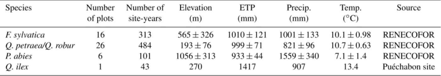
Table 1.Climatic features of the studied sites. ETP is annual Penman–Monteith potential evapotranspiration, Precip. is annual precipitation, and Temp. is annual temperature. Values are site averages±SD among sites.
Species Number Number of Elevation ETP Precip. Temp. Source
of plots site-years (m) (mm) (mm) (◦C)
F. sylvatica 16 313 565±326 1010±121 1001±133 10.1±0.98 RENECOFOR
Q. petraea/Q. robur 26 484 193±76 999±71 821±96 10.7±0.63 RENECOFOR
P. abies 6 101 1056±313 933±44 1559±340 7.1±1.4 RENECOFOR
Q. ilex 1 43 270 1417 907 13.4 Puéchabon site
2013) and induce different growth determinants among taxa (Genet et al., 2010).
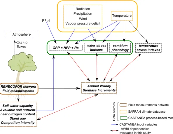
There is a gap between the knowledge obtained from global studies of universal C allocation rules in forests and our understanding of the cell processes that underlie cambial activity; currently, this gap appears to be the primary obstacle to a more complete understanding of wood growth drivers. In this regard, species-specific studies that evaluate the dy-namic of C partitioning to annual wood growth along soil and climate gradients would be highly useful but are lack-ing. Unfortunately, there is a scarcity of data sets that com-bine EC and growth measurements at the same sites (Luys-saert et al., 2007). Here, we circumvented this limitation by complementing stand and soil measurements at a French per-manent plot network of 49 forest sites with process-based simulations of annual and seasonal tree C balance (Fig. 1). Simulations were performed using a process-based model (CASTANEA, Dufrêne et al., 2005) that was thoroughly val-idated using EC data from throughout Europe (Davi et al., 2005; Delpierre et al., 2009, 2012) and was applied using site-specific parameters. By relating biometric measurements to variables that explain the C source and sink activity, we evaluated the key drivers of the annual C allocation to stand wood growth in five species that are representative of the main European forest biomes:Fagus sylvatica,Quercus pe-traeaandQuercus roburfor temperate deciduous broadleaf forests; Picea abies, for high-latitude and high-altitude ev-ergreen needleleaf forests; and Quercus ilex, an evergreen broadleaf species from Mediterranean forests. Specifically, the relative influence of annual and seasonal (from 1 month to 1 year) tree C balance (source control), direct environmen-tal control (water and temperature effects on sink activity) and allocation adjustments related to age, past climate con-ditions, competition intensity and soil nutrient availability on tree growth were considered (Fig. 1). We aimed to (1) quan-tify the relative contributions of source and sink controls to the spatio-temporal dynamic of forest wood growth across a wide range of environmental contexts and (2) provide infor-mation that can be used to refine the representation of forest growth causalities in TBMs.
2 Materials and methods
We based our analyses on three complementary data sources: field measurements, climatic variables from atmospheric re-analysis (Vidal et al., 2010) and process-based simulation data. This hybrid approach allowed us to assess and disen-tangle the effects of previously reported environmental and endogenous drivers of C allocation to wood growth (Fig. 1). 2.1 Study sites and field data
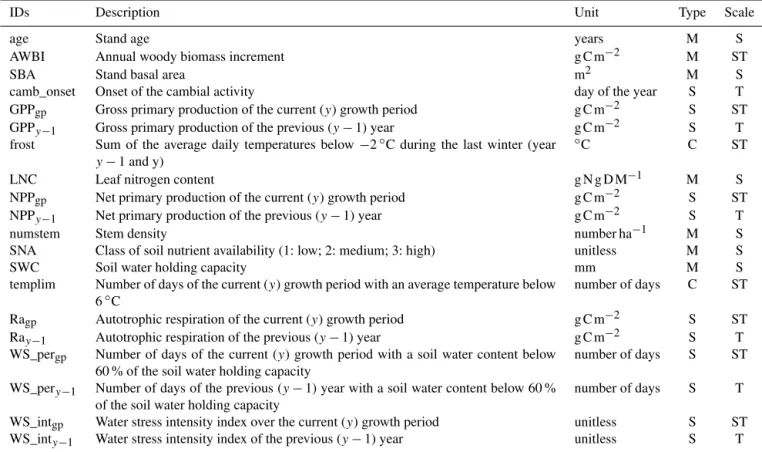
We gathered field measurements from 48 plots from the French Permanent Plot Network for the Monitoring of Forest Ecosystems (RENECOFOR; Ulrich, 1997) and the Puéch-abon tower flux site (Martin-StPaul et al., 2013). The loca-tion and general climatic features of these plots are shown in Fig. 2 and Table 1. Complete site description is available in Supplement S1.
2.1.1 Growth measurements and historical stand growth reconstruction
Growth measurements were obtained via two methods. The first method was dendrochronological sampling, in which 12 to 30 overstorey trees per plot were cored to the pith at breast height with an incremental borer. Cores were collected in 1994 at the RENECOFOR sites and in 2008 at the Puéch-abon site (Lebourgeois, 1997; J. M. Ourcival, unpublished data). Tree circumferences at breast height (CBHs) and total heights were also measured. The average stand age was in-ferred from the tree ring series. The second method was for-est inventories, in which extensive CBH surveys were con-ducted in a 0.5 ha area of every plot (Cluzeau et al., 1998; Gaucherel et al., 2008; J. M. Ourcival, unpublished data).
Tree ring series were combined with the CBH surveys to reconstruct the historical CBHs of every tree on the plots (over 8 to 43 years, Supplement S1). The entire stand tree CBH distribution was reconstructed from the CBHs of the sampled trees using an empirical tree competition model (Deleuze et al., 2004). This model stipulates that only trees with a CBH above a given threshold (σ, the minimum
CASTANEA process-based model SAFRAN climate database
RENECOFOR network field measurements
Atmosphere
fluxes
CO2
GPP = NPP + Ra water stressindexes phenologycambium stress indexestemperature
Radiation
Temperature Precipitation
Wind Vapour pressure deficit
Soil water capacity Available soil nutrient Leaf nitrogen content
Stand age Competiton intensity
Annual Woody Biomass Increments
AWBI dependencies evaluated in this study CASTANEA input variables
Field measurements network
] [CO2
Da
ta
so
ur
ce
s
H2O /
Figure 1.The conceptual framework and the three sources of data (field measurements, climate reanalysis and process-based simulations) used in the analyses.
according to a slope coefficient, γ. Following the work of
Guillemot et al. (2014), the model was calibrated annually, beginning at year (n) of the core sampling and used
itera-tively to reconstruct the past stand CBH growth. Theσ
pa-rameter was first defined using an empirical relationship with the maximum CBH of the stand tree distribution from year (n). Theγ parameter was then adjusted using the tree rings
measured on the sampled trees in year (n−1). The
parame-terized model was finally used to predict the basal area incre-ments of all the trees in the distribution, and consequently the tree CBH distribution in the year (n−1). A detailed
descrip-tion of the iterative process can be found in Supplement S2 and in Guillemot et al. (2014).
The inferred past trajectory of the stand CBH distribution was used to calculate the historical number of stems (num-stem, Table 2) and stand basal area, which we considered to be a proxy for within-stand competition intensity (SBA, Table 2; Kunstler et al., 2011). The historical total woody stand biomass was also calculated (Supplement S3) using species-specific tree-level allometric functions (Bontemps et al., 2009, 2012; Dhôte and Hercé, 1994; Seynave et al., 2005; Vallet et al., 2006) and wood density models (Bouriaud et al., 2004; Wilhelmsson et al., 2002; Zhang et al., 1993). For Q. ilex, we used the appropriate function from Rambal et al. (2004) to calculate the stand woody biomass from CBHs.
Past annual woody biomass increments (AWBIs) were then inferred (Supplement S4).
2.1.2 Measurements of stand characteristics
The stand measurements included the soil water holding ca-pacity (SWHC), leaf area index (LAI), leaf N content (LNC) and soil nutrient availability (SNA). The SWHC was esti-mated via the soil depth and texture measured at two soil pits per plot (Brêthes and Ulrich, 1997). The LAI was estimated from litter collection (Pasquet, 2002), and the sunlit LNC was determined annually for eight trees between 1993 and 1997 (Croisé et al., 1999).
Table 2.Description of the explanatory variables considered in the analyses. The type category indicates the source of the data: measurement (M), SAFRAN climate database (C) or CASTANEA simulations (S). Scale categories indicate the variables considered in spatial (S) and/or temporal (T) analyses.
IDs Description Unit Type Scale
age Stand age years M S
AWBI Annual woody biomass increment g C m−2 M ST
SBA Stand basal area m2 M S
camb_onset Onset of the cambial activity day of the year S T
GPPgp Gross primary production of the current (y) growth period g C m−2 S ST
GPPy−1 Gross primary production of the previous (y−1) year g C m−2 S T
frost Sum of the average daily temperatures below−2◦C during the last winter (year y−1 and y)
◦C C ST
LNC Leaf nitrogen content g N g D M−1 M S
NPPgp Net primary production of the current (y) growth period g C m−2 S ST
NPPy−1 Net primary production of the previous (y−1) year g C m−2 S T
numstem Stem density number ha−1 M S
SNA Class of soil nutrient availability (1: low; 2: medium; 3: high) unitless M S
SWC Soil water holding capacity mm M S
templim Number of days of the current (y) growth period with an average temperature below 6◦C
number of days C ST
Ragp Autotrophic respiration of the current (y) growth period g C m−2 S ST
Ray−1 Autotrophic respiration of the previous (y−1) year g C m−2 S T
WS_pergp Number of days of the current (y) growth period with a soil water content below 60 % of the soil water holding capacity
number of days S ST
WS_pery−1 Number of days of the previous (y−1) year with a soil water content below 60 % of the soil water holding capacity
number of days S T
WS_intgp Water stress intensity index over the current (y) growth period unitless S ST
WS_inty−1 Water stress intensity index of the previous (y−1) year unitless S T
2.2 Climate data
The following meteorological variables at the hourly tempo-ral scale (with 8 km spatial resolution) were obtained from the SAFRAN atmospheric reanalysis (Vidal et al., 2010): global radiation, rainfall, wind speed, air humidity and air temperature. Temperature, which was related to the average altitudes of the SAFRAN cells, was corrected using plot-specific elevation measurements (assuming a lapse rate of 0.6◦K per 100 m, Supplement S1). These variables were
used for climate forcing in the CASTANEA model (Dufrêne et al., 2005; see the following section). In addition, two an-nual temperature indices were used as proxies of winter frost damage and low temperature stress during the growing pe-riod (frost and templimgp, respectively, Table 2).
2.3 Process-based simulation data
We used the CASTANEA model to simulate an ensemble of diagnostic variables that are related to the C source and sink activity of forest stands: the elementary components of the tree C balance, bioclimatic water stress indices and the onset of the biomass growth. The eco-physiological process-based CASTANEA model aims to simulate C and water fluxes and stocks of a monospecific, same-aged forest stand on a
rota-tion timescale. The hourly stand–atmosphere C fluxes pre-dicted by the CASTANEA model have been thoroughly val-idated using EC data from throughout Europe (Davi et al., 2005; Delpierre et al., 2009, 2012). Importantly, the bio-physical hypotheses that were formalized in this model are able to reproduce the interplay of the complex mechanisms that leads to inter-annual variability in the stand C balance (Delpierre et al., 2012); modelling this interplay has been recognized as a substantial challenge for TBMs (Keenan et al., 2012). A complete description of CASTANEA is pro-vided in Dufrêne et al. (2005), and subsequent modifications are described in Davi et al. (2009) and Delpierre et al. (2012). For the purpose of the present study, CASTANEA was pa-rameterized with site-specific SWHC and LNC values. The measured LAI and total woody biomass were used to initial-ize the model simulations. The model’s ability to reproduce the annual variability in LAI and the forest growth has been recently validated (Guillemot et al., 2014). Nevertheless, the annual standing woody biomass was forced to conform to the observed values, because the model was used for diagnostic purposes in this study.
10°W
0 - 200m 200 - 400m 400 - 1000m
1000 - 2000m > 2000m
Elevation
Q. petraea Q. robur
Permanent Plot
F. sylvatica
P. abies
Q. ilex
20°W
10°E 0°
40°N 50°N 58°N
Figure 2.Locations of the study sites.
1. The elementary components of the tree C balance. These components included the GPP, autotrophic respi-ration (Ra) and net balance (i.e. net primary productiv-ity, NPP=GPP – Ra). For a given year y, we aggregated
the hourly simulated C fluxes over different seasonal time periods, with starting days that ranged from 30 to 190 and ending days that ranged from 190 to 350, at a 2-day resolution. The C fluxes were also summed (i) for the species-specific biomass growth periods reported in the literature (GPPgp, Ragpand NPPgp; Supplement S6) and (ii) for the entire preceding year (y−1) as a proxy
of the forest C status induced by past climate conditions (lagged effect, GPPy−1, Ray−1and NPPy−1).
2. Bioclimatic water stress indices. These indices included the intensity and duration of water stress (WS_intgp and WS_pergp, respectively; Supplement S7) during species-specific growing periods that have been re-ported in the literature (Supplement S6). The CAS-TANEA model simulated the daily soil water balance, based on a bucket soil sub-model with two layers (a top soil layer and a total soil layer that includes the top soil layer; Dufrêne et al., 2005). WS_intgpwas then used to quantify the intensity of water stress by summing the reduc index on a daily basis (Granier et al., 1999). reduct = max
0,min
1, SWCt−SWCwilt
0.4×(SWCfc−SWCwilt)
,
where SWCt is the soil water content on dayt (mm),
SWCwilt is the soil water content at the wilting point
(mm) and SWCfc is the soil water content at field ca-pacity (mm).
WS_pergpis the number of days of the current growth period during which the soil water content was less than 60 % of the soil water holding capacity (Table 2, modi-fied from Mund et al., 2010). Water stress indices were also calculated for the entire preceding year (lagged ef-fect of water stress, WS_inty−1and WS_pery−1).
3. The onset of the biomass growth(camb_onset). We used a new growth-onset module (David, 2011; N. Delpierre and N. K. Martin-StPaul, unpublished results) based on a temperature sum trigger (Supplement S8).
2.4 Statistical analyses 2.4.1 General overview
Statistical analyses were conducted in three complementary steps for each studied species. (1) We calculated the correla-tion of the AWBIs and the C fluxes (GPP, NPP and Ra) agggated seasonally (from 1 month to 1 year) to evaluate the re-lationship between the C supply and annual biomass growth changes. (2) The dependences of the AWBIs on the C source and the sink activity were evaluated on an inter-site spatial scale to determine the influence of the site characteristics on biomass growth. The relationship between the age and C al-location to woody biomass was also evaluated in this step. By using the age differences among sites, our chronosequence included a large range of ages (including stands that ranged in age from approximately 30 to 150 years old, Table S1 in Supplement). (3) Finally, the drivers of AWBI were assessed temporally to determine the factors that were responsible for variability in the inter-annual biomass growth.
Because many environmental factors affect both forest sink and source activities, there may be strong covariance among the tree C balance and proxies of environmental stress (Fatichi et al., 2014) that could hamper the inferen-tial power of classical statistical tests (Graham, 2003). How-ever, the explanatory variables used in this study gener-ally had correlation coefficients of less than 0.7, the level above which collinearity begins to severely affect model per-formance (Dormann et al., 2013). One exception was the correlation of components of the tree C balance (because NPP=GPP−Ra). Consequently, the tree C balance
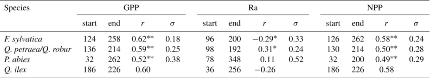
Table 3.Relationships of annual wood growth and the components of the seasonal forest carbon balance: NPP, GPP and Ra. The start and end terms (day of the year) indicate the carbon flux period that yielded the maximum value for the median of the growth-flux correlations among sites. Therterm is the maximum obtained for the median of the site-specific Pearson correlation coefficients; values that are significantly different from 0 are indicated (∗ indicates
P <0.05 and∗∗ indicatesP <0.001). The σ term is the standard deviation of the Pearson correlation values among sites.
Species GPP Ra NPP
start end r σ start end r σ start end r σ
F. sylvatica 124 258 0.62∗∗ 0.18 96 200 −0.29∗ 0.33 126 262 0.58∗∗ 0.24
Q. petraea/Q. robur 136 214 0.59∗∗ 0.25 98 192 0.31∗ 0.24 130 214 0.50∗∗ 0.28
P. abies 32 262 0.52∗∗ 0.38 78 348 0.11 0.52 32 200 0.49∗∗ 0.29
Q. ilex 186 226 0.60 36 256 −0.26 186 226 0.58
Team 2013) using the packages lme4 (Bates et al., 2007), randomForest (Liaw and Wiener, 2002) and MuMIn (Barton and Barton, 2014). Because Quercus petraea andQuercus roburare difficult to distinguish in the field and have a high hybridization rate (Abadie et al., 2012), these two species were grouped in the analyses and are hereafter collectively referred to as “temperate oaks”.
2.4.2 Correlations between growth and C fluxes Pearson correlations between the AWBIs and simulated C fluxes in different seasonal time periods were calculated sep-arately for each site. The highest median correlation value for each species was retained and tested against zero us-ing Wilcoxon signed-rank tests. Critical correlations (i.e. the threshold values for a significant difference with the retained maximum correlation) were determined to evaluate the sen-sitivity of the correlation values to changes in the C flux ag-gregation periods.
2.4.3 Drivers of spatial variations in biomass growth The drivers of spatial variations in biomass growth were evaluated using multiple-regression models using an information-theoretic approach (Burnham and Anderson, 2002). The AWBIs and the considered explanatory variables were averaged for each plot. The variables introduced into the linear models were centred and scaled such that their nor-malized coefficient estimates indicated the relative influence of the predictors on the AWBI. The elementary components of tree C balance (NPP, GPP and Ra) were introduced one at a time into the models. For each species, multiple-regression models that contained all possible combinations of the ex-planatory variables were fitted. The models were compared using the second-order Akaike information criterion (AIC), and all models with an Akaike weight of at least 1 % of the best approximating (lowest AIC) model were considered to be plausible (Burnham and Anderson, 2002). Ultimately, we retained the variables that appeared in at least 95 % of the selected models. Models fitted using P. abiesdata were re-stricted to a maximum of three explanatory variables because
of the small sample size (n=6, Table 1). Q. ilex (n=1)
was not considered in the spatial analyses. The uncertainty of the simulated C fluxes was assessed in the analyses us-ing a bootstrap procedure (Chernick, 2011): all linear mod-els were fitted 1000 times, and at each iteration, the C flux values were randomly sampled within the root-mean-square error of the CASTANEA simulations (Supplement S9) to ob-tain a parameter estimate distribution for each variable. We finally retained the explanatory variables with parameter esti-mate distributions that excluded the zero value at a two-tailed probability level of 5 %.
2.4.4 Drivers of temporal variations in biomass growth
A temporal analysis was conducted on the standardized AWBI series: a double-detrending process was applied to each series based on an initial linear regression model, fol-lowed by fitting a cubic smoothing spline with a 50 % fre-quency response cut-off (Mérian et al., 2011). For analysing the temporal variations in biomass growth we used an RF learning method (Breiman, 2001), which was possible be-cause of the large sample size (n=931 site-years). The RF
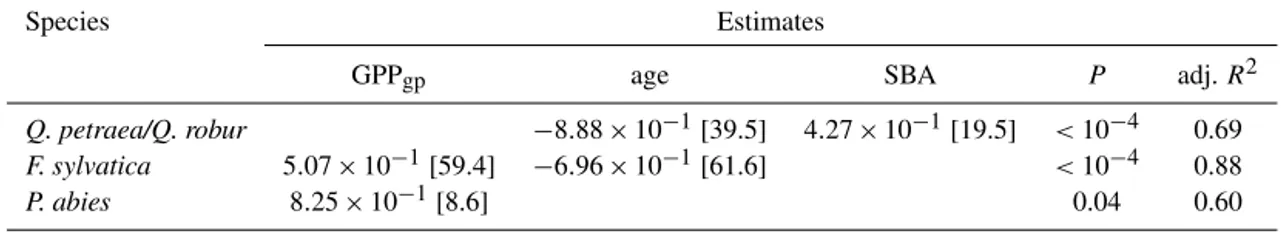
Table 4.Spatial dependences of the annual woody growth: multiple-regression estimates. Data have been centred and scaled. GPPgpis the
gross primary production of the growth period, age is the average age of the stand, and SBA is the stand basal area (Table 2). Values: estimates [Fvalues]. All estimate values differed significantly from 0 (P <0.001). All variables were retained in the bootstrap procedure (see main text).
Species Estimates
GPPgp age SBA P adj.R2
Q. petraea/Q. robur −8.88×10⁻¹[39.5] 4.27×10⁻¹[19.5] <10−4 0.69
F. sylvatica 5.07×10⁻¹[59.4] −6.96×10⁻¹[61.6] <10−4 0.88
P. abies 8.25×10⁻¹[8.6] 0.04 0.60
square error when a given variable was randomized in the validation subsamples. The forms of the dependences were illustrated by partial dependence plots (graphical depiction of the marginal effect of a given variable; Cutler et al., 2007). We used this information (variable selection and dependence forms) to test for the significance of the temporal AWBI de-pendences within the linear model. The uncertainty in the simulated C fluxes was considered in the linear models, fol-lowing the procedure described in the spatial analysis sec-tion.
3 Results
3.1 Relationship between woody biomass growth and C fluxes
The elementary components of the simulated seasonal tree C balance differed in terms of their relationships with the inter-annual variability of the annual woody biomass incre-ments (AWBI, Table 3). The simulated seasonal GPP and NPP were linked to AWBIs with a comparable agreement between species. However, the simulated Ra had weak and often non-significant relationships with the AWBIs across the 49 studied plots. The strongest correlations were obtained for flux aggregation periods that (i) were generally consistent within a species for GPP and NPP but different for Ra and (ii) strongly differed among species (Table 3). The coefficients of variation of the simulated annual NPP, GPP and Ra across the 49 studied sites were 10.8±3, 7.4±2 and 6.8±3 %,
re-spectively. GPP and NPP were summed from the beginning of May to the beginning of August and September, in temper-ate oaks andF. sylvatica, respectively. The longest GPP and NPP aggregation periods were obtained for P. abies (from the beginning of February to mid-September), and the short-est period were found forQ. ilex(from the beginning of July to mid-August). Minor (less than 20 days) changes in the flux aggregation period associated with the maximum simulated flux–AWBI correlation usually marginally affected the corre-lation values (Supplement S10). Consequently, aggregation periods that were less than 13 days different (either in terms of their starting or ending dates) from the values reported
in Table 3 were generally not significantly lower than the maximum values (see the critical values presented in Sup-plement S10).
3.2 Spatial dynamic of C allocation to woody biomass growth
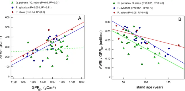
The inter-site variability in biomass growth was well explained by the selected multiple-regression models (R2>0.6). We highlighted that species varied in terms of
their inter-site dependences (Table 4). The simulated C sup-ply during the growth period (GPPgp, Table 2) was positively correlated with biomass growth inF. sylvaticaandP. abies, whereas there was no significant relationship between the average AWBI and photosynthesis among sites for temper-ate oaks (Fig. 3a). Notably, the final models did not include NPPgp or Ragp for any species. The stand age was an im-portant driver of biomass growth in temperate oaks andF. sylvatica. The stand age explained a substantial portion of the AWBI : C supply ratio in all species, although the rela-tionship was not significant forP. abies(Fig. 3b). The frac-tion of C sequestered in woody biomass decreased with stand age (Table 4, Fig. 3b) and was reduced by half in temperate oaks andF. sylvaticastands that were between 50 and 150 years of age (from 0.3 to 0.13 and from 0.25 to 0.1, respec-tively). Additionally, we identified a significant and positive effect of stand basal area on both AWBI (Table 4) and the AWBI : GPPgpratio (data not shown) in temperate oaks. 3.3 Temporal dynamic of carbon allocation to woody
biomass growth
50 100 150 0
0.05 0.10 0.15 0.20 0.25 0.30
1100 1200 1300 1400 1500 1600 1700 1800
0 100 200 300 400 500
600
A
B
Q. petraea / Q. robur (P=0.6, R²=0.01) F. sylvatica (P<0.001, R²=0.41) P. abies (P=0.04, R²=0.6)
Q. petraea / Q. robur (P<0.001, R²=0.46) F. sylvatica (P<0.001, R²=0.76) P. abies (P=0.09, R²=0.43)
stand age (year) GPP (gC/m²)
A
W
B
I (
gC/
m
²)
A
W
B
I /
G
P
P
(un
itle
ss)
gp
gp
Figure 3.Spatial dependences of annual wood growth.(a)Relationship of the AWBI and the GPP of the growth period (GPPgp) averaged
over sites.(b)Age-related decline of the C partitioning to AWBI (AWBI/GPPgp).
Table 5.Temporal dependences of the annual woody growth: multiple-regression estimates. Data have been centred and scaled. GPPgpis
the gross primary production of the growth period, WS_pergp is a water stress index of the growth period, WS_inty−1is a water stress index of the previous year, templim is a low temperature index of the growth period (Table 2).D1 andD2 are dummy variables (D1=0 if GPPgp<1400 g C m−2,D1=1 otherwise;D2=0 if GPPy−1<1550 g C m−2,D2=1 otherwise; see Fig. 5).ρis the parameter of the first-order autoregressive process used to model the temporal autocorrelation of within-stand errors. Values: estimates [Fvalues]. Estimate values differing from 0 are indicated (∗
P <0.05,∗∗P <0.01,∗∗∗P <0.001). The estimate with a1index indicates variable not retained in the bootstrap procedure (see main text).
Estimates Species
Q. petraea/ F. sylvatica P. abies Q. ilex
Q. robur
GPPgp 3.26×10⁻¹∗∗∗ 4.87×10⁻¹∗∗∗ 2.4×10−1∗[3.5]
WS_pergp −1.09×10⁻¹∗∗ −2.04×10⁻¹∗∗∗ −5.8×10⁻¹∗∗∗
WS_inty−1 −2.37×10⁻¹∗∗∗ −2.2×10−1∗[6.3]
GPPy−1 3.82×10−1∗[3.3] −4×10⁻¹∗∗[3.2]
templim −9.60×10⁻²∗∗1 −1.26∗∗∗[3.5]
D1 −2.4×10⁻¹∗∗∗
D2 −3.9×10⁻¹∗∗[0.8]
D1·GPPgp 1.33∗∗[8.2]
D2·GPPy−1 −4×10⁻¹∗∗[6.4]
ρ 0.61 0.68 0.52 0.44
P <10−4 <10−4 7.7×10⁻³ <10−4
adj.R2 0.21 0.42 0.20 0.43
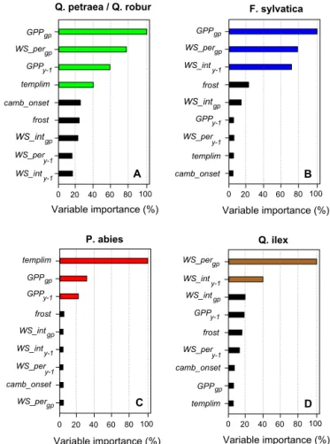
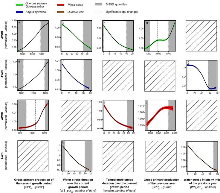
was the predominant driver of the AWBI variability of Q. ilex, and was also strongly related to growth in temperate deciduous species. Low temperatures during the growth pe-riod (templimgp) most substantially affectedP. abiesand also explained a portion of the variability in AWBI of temper-ate oaks. The simultemper-ated wtemper-ater and temperature stress indices had negative and quasi-linear marginal effects on the AWBI
(Fig. 5). Finally, environmental lagged effects contributed substantially to the AWBI variability in all species: the wa-ter stress intensity of the previous year (WS_inty−1) affected
the growth ofF. sylvaticaandQ. ilex, whereas the simulated C supply of the previous year (GPPy−1) affected temperate
ef-templim camb_onset GPP WS_per WS_int
A B
C D
0 20 40 60 80 100
0 20 40 60 80 100 0 20 40 60 80 100
0 20 40 60 80 100
F. sylvatica Q. petraea / Q. robur
P. abies Q. ilex
frost GPPgp
WS_pergp WS_inty-1
gp
y-1
y-1
GPPgp
WS_pergp GPPy-1
WS_intgp WS_pery-1 WS_inty-1
GPPgp
GPPy-1
WS_intgp WS_inty-1 WS_per
y-1
WS_pergp camb_onset
camb_onset templim
templim frost
frost
WS_pergp
WS_inty-1 WS_intgp GPPy-1
frost WS_pery-1 camb_onset
GPPgp
templim
Variable importance (%) Variable importance (%)
Variable importance (%) Variable importance (%)
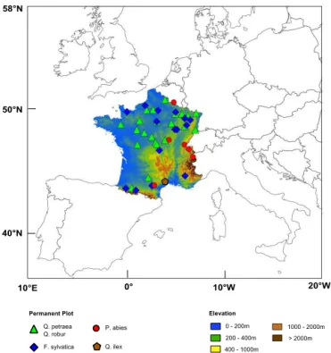
Figure 4.Temporal dependences of annual wood growth: the roles of explanatory variables from RF classification. Variable impor-tance is expressed as the percentage of the imporimpor-tance of the top-ranked explanatory variable. The variable identifiers (IDs) are listed in Table 2. The coloured variables were retained in subsequent anal-yses.
fect on AWBI only under high water stress or low C supply (Fig. 5). The effects of the retained variables (Fig. 4) were evaluated via multiple-regression models that used dummy variables to test for the significance of slope changes when thresholds appeared on partial plots (Fig. 5). The models ex-plained approximately 20 % of the variability in the AWBI for temperate oaks andP. abies, and approximately 40 % of the variability for F. sylvaticaandQ. ilex (Table 5). All of the explanatory variables had significant effects, buttemplim was not retained in the models for temperate oaks after the bootstrap procedure that accounted for the uncertainty of the C flux simulations. We observed significant changes in the slopes of the effect of GPPy−1on temperate oaks and the
ef-fect of GPPgponP. abies(Table 5). The models with NPPgp and NPPy−1variables revealed the same AWBI dependences
as the models described above, but with reduced explanatory power. The models with Ragpand Ray−1variables were not
significant (data not shown).
4 Discussion
This study quantified the C that is allocated annually to the woody biomass increment for five species that are repre-sentative of the main European forest biomes. By comple-menting field measurements from a permanent plot network with process-based modelling, our approach circumvented the limitation of EC data scarcity and characterized the an-nual partitioning of C into woody biomass at 49 sites over France (931 site-years). We were thus able to identify the species-specific drivers of the spatio-temporal dynamics of the allocation of C to wood growth along ecological gradi-ents.
4.1 The correlation between the tree C balance and woody biomass growth
a b c d
e f g
h i
l 0 10 20 30 40 50 0 4 8 12 16 20 1200 1600 2000
0 20 40 60 80 0 20 40 60 80
0 20 40 60 80 100 0 20 40 60 80
0 10 20 30 40 50 60 1000 1500 2000 2500
1.00 1.05 1.10 0.95 1.0 1.1 1.2 0.9 0.8 0.7 1.0 0.9 1.1 1.000 1.005 1.010 1.995 1.00 1.05 1.10 0.95 0.90 0.96 1.00 1.04 1.08 0.94 0.98 1.02 1.06 0.92 0.96 1.00 1.04 0.8 1.0 1.2 0.92 0.96 1.00 0.95 0.97 0.99 0.96 1.00 1.04 5-95% quantiles Temperature stress duration over the current
growth period
[templim, number of days]
AW BI [nor m ali zed - un itle ss ] AW BI [nor m ali zed - un itle ss ] AW BI [nor m ali zed - un itle ss ] AW BI [nor m ali zed - un itle ss ] Quercus petraea Fagus sylvatica Picea abies Quercus ilex k j
1000 1400 1800
1000 1300 1600
significant slope changes
800 1300 1800
Gross primary production of the current growth period
[GPP , gp gC/m²]
Water stress duration over the current
growth period
[WS_per , gp number of days]
Gross primary production of the previous year
[GPP , y-1 gC/m²]
Water stress intensity index of the previous year
[WS_int , unitless]y-1 Quercus robur
Figure 5.Temporal dependences of annual wood growth: marginal effects of each explanatory variable on the annual wood growth. The lines represent smoothing splines with 50 % frequency response cut-offs. The coloured areas indicate the 95 % confidence intervals. The 5 and 95 % data quantiles (grey areas) were not considered in the discussion. The marginal effect of a given variableXwas obtained by fixing the value ofXand averaging the RF predictions over all the combinations of observed values for the other predictors in the data set (Cutler et al., 2007). The marginal predictions were collected over the entire range ofXin the training data using a regular grid.
annual growth and a short period of C flux aggregation in early summer that was reported for Q. ilex corresponds to the effect of growth cessation on the annual biomass incre-ment, which has been attributed to a drought-induced limi-tation of cambial activity at the Puéchabon site (Lempereur et al., 2015). The processes that underlie the relationship of the long flux aggregation period and the annual biomass in-crement ofP. abiesmay include the effect of late winter tem-perature on cambium phenology (Rossi et al., 2011). Overall, our results suggest that using growth-flux correlation coeffi-cients when investigating either source limitation of growth
or the seasonality of C allocation to woody biomass can lead to misleading conclusions.
4.2 Between-site variability in the C allocation to woody biomass growth is related to ontogeny and competition intensity
are associated with increases in the hydraulic resistance of xylem, which may lead to declines in the turgor of living cells and result in potentially negative consequences on cambial activity (Woodruff et al., 2004). This constraint may result in a height-related sink limitation of growth (Woodruff and Meinzer, 2011), which is consistent with our results. Addi-tionally, life-history traits, such as a greater emphasis on re-production in older stands, could also be involved. However, the interactions of growth and reproductive mechanisms are still under debate (Hoch et al., 2013; Thomas, 2011) and have yet to be properly represented in TBMs. Only the GPP com-ponent of the simulated tree C balance was retained in the final models (Table 4), thereby indicating that an increase in maintenance respiration with greater stand biomass most likely did not contribute to the age-related decline in biomass growth (Drake et al., 2011; Tang et al., 2014). Although height-related hydraulic constraints on C assimilation have been suggested to be an important driver (Ryan et al., 2006; Tang et al., 2014), recent studies have suggested that changes in demography and stand structure may primarily explain the age-related decline observed in stand wood growth (Bink-ley et al., 2002; Xu et al., 2012). Our results suggest that changes in the C allocation should also be considered, be-cause no mortality occurred in our plots during the measure-ment period (data not shown). We additionally identified a significantly higher C partitioning to woody biomass in tem-perate oak stands with greater competition intensity (i.e. high stand basal area, Table 3). To date, reports regarding the ef-fect of competition on C allocation dynamics are conflict-ing (Litton et al., 2007) and suggest no significant or consis-tent effect. Moreover, we found no significant effect of soil nutrient availability on the C allocation dynamics along the studied ecological gradient, whereas a recent meta-analysis reported that this factor positively affects C partitioning to forest biomass on the global scale (Vicca et al., 2012). The RENECOFOR network only includes relatively fertile sites (Supplement S5), which could putatively explain the appar-ent tension between our results and the conclusions of the meta-analysis. Therefore, more studies are required to eluci-date the contributions of the various drivers to the variation in C partitioning to woody biomass on scales that range from local to global.
4.3 Inter-annual variability in woody biomass growth is consistent with combined source–sink limitations Water and temperature stress exerted significant direct con-trol on the inter-annual variation of woody biomass growth (i.e. independent of their effects on C assimilation) for ev-ery species and biome (Table 5 and Figs. 4 and 5). Cam-bial growth has been reported to be inhibited at lower water stress levels than photosynthesis (Muller et al., 2011; Tardieu et al., 2011). Indeed, drought-induced decrease in cell tur-gor strongly affects cell divisions (Woodruff and Meinzer, 2011) and cell wall expansion (Cosgrove, 2005; Lockhart,
1965) before gas exchange modulation comes into play. Sim-ilarly, there is evidence that cell growth processes, such as cell division, are more sensitive than photosynthesis to low temperatures (Körner, 2008). Although these findings docu-mented the plausible mechanisms of sink control of biomass growth at the cellular scale, there is still considerable debate regarding whether the sink or the C source actually limits the growth of the world’s forests (Palacio et al., 2014; Wiley and Helliker, 2012). The typically observed large C reserve pools (Hoch et al., 2003; Würth et al., 2005) have been interpreted as a consequence of an overabundant C supply and thus ev-idence of sink control of tree growth (Körner, 2003). How-ever, recent works have suggested that a source limitation of growth may be compatible with large C reserve pools if part of this mobile C is sequestered rather than stored (Millard and Grelet, 2010) or if C storage is an active tree response to environmental stress (Dietze et al., 2014; Wiley and Helliker, 2012). Using an alternative methodology (i.e. a methodology that is not based on C storage measurement) our results sug-gest that sink limitation has a significant effect on the annual woody biomass growth of five species that are representative of different European biomes, including deciduous temperate forests. Because sink limitation implies that there are peri-ods with significant C supply but no growth, our results also corroborate recent empirical studies that reported a signifi-cant role of growth duration in the annual variability of tree radial increment (Brzostek et al., 2014; Cuny et al., 2012; Lempereur et al., 2015). Additionally, we observed that past environmental constraints significantly affected C partition-ing to wood growth for each species and biome (Table 5 and Figs. 4 and 5). The lagged effect of the previous year’s low C supply (GPPy−1) possibly indicates a preferential C
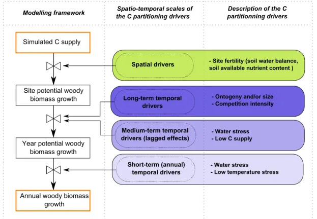
Simulated C supply
Site potential woody biomass growth
Spatial drivers
Medium-term temporal drivers (lagged effects)
Long-term temporal drivers
Short-term (annual) temporal drivers
Spatio-temporal scales of the C partitioning drivers
Modelling framework partitionning driversDescription of the C
- Water stress
- Low temperature stress - Ontogeny and/or size - Competition intensity
- Water stress - Low C supply
- Site fertility (soil water balance, soil available nutrient content )
Year potential woody biomass growth
Annual woody biomass growth
Figure 6.Modelling framework for a combined source- and sink-driven representation of C allocation to wood growth.
was most closely related to the annual variability in growth; this result indicates GPP’s important role in explaining the annual variability in the net ecosystem productivity of Eu-ropean forests (Delpierre et al., 2012). Overall, our findings support the premise that forest woody biomass growth is sub-ject to complex control processes that include both source and sink limitations, following Liebig’s law: although nu-merous processes potentially influence wood growth, stand growth at a given site and a given year is predominantly lim-ited by the most constraining factor. C (source) limitation of growth can thus only occur when other factors are non-limiting (Fatichi et al., 2014), a situation that is expected to be rare in strongly constrained environment such as Mediter-ranean or mountainous areas (Fig. 4).
4.4 Toward an integrated modelling framework
Most models that are currently used to project the outcome of global changes on forests represent wood growth as a frac-tion of the total C uptake (i.e. source control of growth; De Kauwe et al., 2014). This C-centric perspective overlooks the possibility of sink control of growth and thus ignores results such as those presented in this study and those of earlier lo-cal studies (reviewed by Fatichi et al., 2014). Consequently, this perspective possibly hampers the ability of TBMs to project future forest productivity (Fatichi et al., 2014). On the basis of our analysis of the spatio-temporal dynamics of
Our approach can be seen as an intermediate step toward a more mechanistic representation of C allocation to woody biomass (Hölttä et al., 2010; Schiestl-Aalto et al., 2015). It synthesizes the current knowledge regarding forest growth dependences and has the potential to unify seemingly con-tradictory observations within a single modelling framework. The simulated growth is indeed subject to the combined con-trols of C supply and changes in C allocation due to endoge-nous adjustments and/or modulations of sink activity (Fig. 6). These controls result from distinct processes, which are inde-pendently represented in the modelling framework. The rel-ative influences of the various processes, i.e. the simulated growth causalities, are thus likely to vary both spatially and temporally, depending on the environmental conditions faced by trees. Our approach therefore has the potential to shed light on the contrasted results reported by correlative stud-ies. Although the value is comparable to the values of pre-vious studies (Lebourgeois et al., 2005; Mérian et al., 2011), the proportion of the annual growth variability that was ex-plained by our approach was moderate (Table 5). Plausible explanations for this result include (i) unreported manage-ment interventions that may have skewed the historical stand growth reconstruction and (ii) potentially important growth drivers that were not considered here, such as changes in C partitioning due to mast seeding (Mund et al., 2010), genetic differentiation among tree populations (Vitasse et al., 2014) or allometry-mediated tree acclimation to drought (Martin-StPaul et al., 2013). A third factor that hampered the abil-ity of our empirical models to explain the annual growth variability is the potential disagreement between the CAS-TANEA outputs that were used as explanatory variables and the corresponding actual drivers. Although we argued that (i) the CASTANEA model has been thoroughly validated at many EC sites from throughout Europe and (ii) the pre-sented growth dependences demonstrated their robustness against the reported uncertainties of the CASTANEA sim-ulations, the quality of the simulations was limited by the idiosyncrasies of the sites we examined in this study. In par-ticular, a number of past disturbances such as insect out-breaks, windthrow or unreported commercial thinning could have temporarily induced large discrepancies between the actual and simulated C fluxes (Grote et al., 2011; Hicke et al., 2012). The error that is attributable to model perfor-mance unfortunately remains unknown because of the ab-sence of EC measurements at our study sites (except for the Puéchabon site; see Delpierre et al., 2012). Despite this ad-ditional uncertainty, the combined use of field measurements and process-based modelling allowed us to present the first species-specific evaluation of annual C allocation to growth along regional environmental gradients. Our results suggest that implementing the presented C allocation dependences in TBMs will refine the projections of the outcome of global changes on forest growth and have implications for the pre-dicted evolution of forest C sink, forest diebacks and tree species distributions (Cheaib et al., 2012).
The Supplement related to this article is available online at doi:10.5194/bg-12-2773-2015-supplement.
Acknowledgements. We wish to thank the Office National des
Forêts and the RENECOFOR network team, particularly Manuel Nicolas and Marc Lanier, for providing the RENECOFOR database. The SAFRAN database was provided by Météo-France as part of the HYMEX project. J. Guillemot received a PhD grant from the French Ministère de l’Enseignement Supérieur et de la Recherche and the University of Paris-Sud. A post-doctoral research grant to N. K. Martin-StPaul was provided by the Humboldt project within GIS Climat. As part of the ICP forests network data (icp-forests.net), the material used in this article is available, free of charge, upon request (please contact M. Nicolas, [email protected],+00331 60 74 92 28, Office National des Forêts, Fontainebleau, 77300, France).
Edited by: S. Zaehle
References
Abadie, P., Roussel, G., Dencausse, B., Bonnet, C., Bertocchi, E., Louvet, J., Kremer, A., and Garnier-Géré, P.: Strength, diversity and plasticity of postmating reproductive barriers between two hybridizing oak species (Quercus robur L.andQuercus petraea (Matt) Liebl.), J. Evol. Biol., 25, 157–173, 2012.
Archer, K. J. and Kimes, R. V: Empirical characterization of random forest variable importance measures, Comput. Stat. Data Anal., 52, 2249–2260, 2008.
Babst, F., Bouriaud, O., Papale, D., Gielen, B., Janssens, I. A., Nikinmaa, E., Ibrom, A., Wu, J., Bernhofer, C., Köstner, B., Grünwald, T., Seufert, G., Ciais, P., and Frank, D.: Above-ground woody carbon sequestration measured from tree rings is coher-ent with net ecosystem productivity at five eddy-covariance sites, New Phytol., 201, 1289–1303, 2014.
Bansal, S. and Germino, M. J.: Carbon balance of conifer seedlings at timberline: relative changes in uptake, storage, and utilization, Oecologia, 158, 217–27, 2008.
Barbaroux, C., Breda, N., and Dufrene, E.: Distribution of above-ground and below-above-ground carbohydrate reserves in adult trees of two contrasting broad-leaved species (Quercus petraea and Fagus sylvatica), New Phytol., 157, 605–615, 2003.
Barton, K. and Barton, M. K.: Package “MuMIn,” Version, 1, 1–57, 2014.
Bates, D., Sarkar, D., Bates, M. D., and Matrix, L.: The lme4 pack-age, R Packag. version, 2, 1–29, 2007.
Beer, C., Reichstein, M., Ciais, P., Farquhar, G. D., and Papale, D.: Mean annual GPP of Europe derived from its water balance, Geo-phys. Res. Lett., 34, 1–4, 2007.
Binkley, D., Stape, J. L., Ryan, M. G., Barnard, H. R., and Fownes, J.: Age-related Decline in Forest Ecosystem Growth: An Individual-Tree, Stand-Structure Hypothesis, Ecosystems, 5, 58–67, 2002.
Bontemps, J.-D., Herve, J.-C., Duplat, P., and Dhôte, J.-F.: Shifts in the height-related competitiveness of tree species following re-cent climate warming and implications for tree community com-position: the case of common beech and sessile oak as predom-inant broadleaved species in Europe, Oikos, 121, 1287–1299, 2012.
Bouriaud, O., Bréda, N., Le Moguédec, G., and Nepveu, G.: Mod-elling variability of wood density in beech as affected by ring age, radial growth and climate, Trees-Struct. Funct., 18, 264– 276, 2004.
Breiman, L.: Random forests, Mach. Learn., 45, 5–32, 2001. Brêthes, A. and Ulrich, E.: RENECOFOR – Caractéristiques
pé-dologiques des 102 peuplements du réseau., Off. Natl. des forêts, Département des Rech. Tech., 1997.
Brüggemann, N., Gessler, a., Kayler, Z., Keel, S. G., Badeck, F., Barthel, M., Boeckx, P., Buchmann, N., Brugnoli, E., Esper-schütz, J., Gavrichkova, O., Ghashghaie, J., Gomez-Casanovas, N., Keitel, C., Knohl, a., Kuptz, D., Palacio, S., Salmon, Y., Uchida, Y., and Bahn, M.: Carbon allocation and carbon isotope fluxes in the plant-soil-atmosphere continuum: a review, Biogeo-sciences, 8, 3457–3489, doi:10.5194/bg-8-3457-2011, 2011. Brzostek, E. R., Dragoni, D., Schmid, H. P., Rahman, a F., Sims, D.,
Wayson, C. a, Johnson, D. J., and Phillips, R. P.: Chronic water stress reduces tree growth and the carbon sink of deciduous hard-wood forests., Glob. Chang. Biol., 20, 8, doi:10.1111/gcb.12528, 2014.
Burnham, K. P. and Anderson, D. R.: Model selection and multi-model inference: a practical information-theoretic approach, Springer, 2002.
Carnicer, J., Barbeta, A., Sperlich, D., Coll, M., and Peñuelas, J.: Contrasting trait syndromes in angiosperms and conifers are associated with different responses of tree growth to temperature on a large scale, Front. Plant Sci., 4, 409, doi:10.3389/fpls.2013.00409, 2013.
Carvalhais, N., Forkel, M., Khomik, M., Bellarby, J., Jung, M., Migliavacca, M., Mu, M., Saatchi, S., Santoro, M., and Thurner, M.: Global covariation of carbon turnover times with climate in terrestrial ecosystems, Nature, 514, 213–217, 2014.
Chapin, F. S., Schulze, E.-D., and Mooney, H. A.: The ecology and economics of storage in plants, Annu. Rev. Ecol. Syst., 21, 423– 447, 1990.
Cheaib, A., Badeau, V., Boe, J., Chuine, I., Delire, C., Dufrêne, E., François, C., Gritti, E. S., Legay, M., Pagé, C., Thuiller, W., Viovy, N., and Leadley, P.: Climate change impacts on tree ranges: model intercomparison facilitates understanding and quantification of uncertainty., Ecol. Lett., 15, 533–44, 2012. Chen, G., Yang, Y., and Robinson, D.: Allocation of gross primary
production in forest ecosystems: allometric constraints and envi-ronmental responses, New Phytol., 200, 1176–1186, 2013. Chernick, M. R.: Bootstrap methods: A guide for practitioners and
researchers, Wiley, 2011.
Clark, D. B., Mercado, L. M., Sitch, S., Jones, C. D., Gedney, N., Best, M. J., Pryor, M., Rooney, G. G., Essery, R. L. H., Blyth, E., Boucher, O., Harding, R. J., Huntingford, C., and Cox, P. M.: The Joint UK Land Environment Simulator (JULES), model descrip-tion – Part 2: Carbon fluxes and vegetadescrip-tion dynamics, Geosci. Model Dev., 4, 701–722, doi:10.5194/gmd-4-701-2011, 2011. Cluzeau, C., Ulrich, E., Lanier, M., and Garnier, F.: RENECOFOR
– Interprétation des mesures dendrométriques de 1991 à 1995 des
102 peuplements du réseau, Off. Natl. des forêts, Département des Rech. Tech., 322 pp., 1998.
Cosgrove, D. J.: Growth of the plant cell wall, Nat. Rev. Mol. Cell Biol., 6, 850–61, doi:10.1038/nrm1746, 2005.
Croisé, L., Cluzeau, C., Ulrich, E., Lanier, M., and Gomez, A.: RENECOFOR – Interprétation des analyses foliaires réalisées dans les 102 peuplements du réseau de 1993 a 1997 et premières évaluations interdisciplinaires, Off. Natl. des forêts, Département des Rech. Tech., 428 pp., 1999.
Cuny, H. E., Rathgeber, C. B. K., Lebourgeois, F., Fortin, M., and Fournier, M.: Life strategies in intra-annual dynamics of wood formation: example of three conifer species in a temperate forest in north-east France, Tree Physiol., 32, 612–625, 2012. Cutler, D. R., Edwards, T. C., Beard, K. H., Cutler, A., and Hess,
K. T.: Random forests for classification in ecology, Ecology, 88, 2783–2792, 2007.
Daudet, F.-A., Améglio, T., Cochard, H., Archilla, O., and Lacointe, A.: Experimental analysis of the role of water and carbon in tree stem diameter variations, J. Exp. Bot., 56, 135–144, 2005. David, A.: Modélisation de la croissance ligneuse chez le Hêtre et le
Chêne sessile. Master’s thesis dissertation, Université Paris-Sud, Orsay, 2011.
Davi, H., Dufrêne, E., Granier, a., Le Dantec, V., Barbaroux, C., François, C., and Bréda, N.: Modelling carbon and water cycles in a beech forest, Ecol. Modell., 185, 387–405, 2005.
Davi, H., Barbaroux, C., Francois, C., and Dufrene, E.: The fun-damental role of reserves and hydraulic constraints in predicting LAI and carbon allocation in forests, Agric. For. Meteorol., 149, 349–361, 2009.
De Kauwe, M. G., Medlyn, B. E., Zaehle, S., Walker, A. P., Dietze, M. C., Wang, Y., Luo, Y., Jain, A. K., El-Masri, B., and Hickler, T.: Where does the carbon go?, A model–data intercomparison of vegetation carbon allocation and turnover processes at two tem-perate forest free-air CO2 enrichment sites, New Phytol., 203, 883–899, doi:10.1111/nph.12847, 2014.
Deleuze, C., Pain, O., Dhôte, J. F., and Hervé, J. C.: A flexible radial increment model for individual trees in pure even-aged stands, Ann. For. Sci., 61, 327–335, 2004.
Delpierre, N., Soudani, K., François, C., Köstner, B., Pontailler, J.-Y., Nikinmaa, E., Misson, L., Aubinet, M., Bernhofer, C., Granier, a., Grünwald, T., Heinesch, B., Longdoz, B., Ourcival, J.-M., Rambal, S., Vesala, T., and Dufrêne, E.: Exceptional car-bon uptake in European forests during the warm spring of 2007: a data-model analysis, Glob. Chang. Biol., 15, 1455–1474, 2009. Delpierre, N., Soudani, K., François, C., Le Maire, G., Bernhofer, C., Kutsch, W., Misson, L., Rambal, S., Vesala, T., and Dufrêne, E.: Quantifying the influence of climate and biological drivers on the interannual variability of carbon exchanges in European forests through process-based modelling, Agric. For. Meteorol., 154/155, 99–112, 2012.
Delpierre, N., Vitasse, Y., Chuine, I., Guillemot, J., Bazot, S., Rutishauser, T., and Rathgeber, C. B. K.: Temperate and boreal forest tree phenology: from organ-scale processes to terrestrial ecosystem models, Ann. For. Sci., in press, doi:10.1007/s13595-015-0477-6, 2015.
Dietze, M. C., Sala, A., Carbone, M. S., Czimczik, C. I., Mantooth, J. A., Richardson, A. D., and Vargas, R.: Nonstructural Carbon in Woody Plants, Annu. Rev. Plant Biol., 65, 667–687, 2014. Dormann, C. F., Elith, J., Bacher, S., Buchmann, C., Carl, G., Carré,
G., Marquéz, J. R. G., Gruber, B., Lafourcade, B., and Leitão, P. J.: Collinearity: a review of methods to deal with it and a simula-tion study evaluating their performance, Ecography (Cop.)., 36, 27–46, 2013.
Drake, J. E., Davis, S. C., Raetz, L. M., and DeLucia, E. H.: Mech-anisms of age-related changes in forest production: the influence of physiological and successional changes, Glob. Chang. Biol., 17, 1522–1535, 2011.
Drobyshev, I., Gewehr, S., Berninger, F., and Bergeron, Y.: Species specific growth responses of black spruce and trembling aspen may enhance resilience of boreal forest to climate change, J. Ecol., 101, 231–242, 2013.
Dufrêne, E., Davi, H., Francois, C., Le Maire, G., Le Dantec, V., and Granier, A.: Modelling carbon and water cycles in a Beech forest – Part I: Model description and uncertainty analysis on modelled NEE, Ecol. Modell., 185, 407–436, 2005.
Fatichi, S., Leuzinger, S., and Körner, C.: Moving beyond photosyn-thesis: from carbon source to sink-driven vegetation modeling, New Phytol., 201, 1086–1095, doi:10.1111/nph.12614, 2014. Franklin, O., Johansson, J., Dewar, R. C., Dieckmann, U.,
McMur-trie, R. E., Brännström, Å., and Dybzinski, R.: Modeling carbon allocation in trees: a search for principles, Tree Physiol., 32, 648– 666, 2012.
Friend, A. D., Lucht, W., Rademacher, T. T., Keribin, R., Betts, R., Cadule, P., Ciais, P., Clark, D. B., Dankers, R., Falloon, P. D., Ito, A., Kahana, R., Kleidon, A., Lomas, M. R., Nishina, K., Ostberg, S., Pavlick, R., Peylin, P., Schaphoff, S., Vuichard, N., Warsza-wski, L., Wiltshire, A., and Woodward, F. I.: Carbon residence time dominates uncertainty in terrestrial vegetation responses to future climate and atmospheric CO2, Proc. Natl. Acad. Sci., 111, 9, doi:10.1073/pnas.1222477110, 2013.
Gaucherel, C., Guiot, J., and Misson, L.: Changes of the po-tential distribution area of French Mediterranean forests under global warming, Biogeosciences, 5, 1493–1504, doi:10.5194/bg-5-1493-2008, 2008.
Genet, H., Bréda, N., and Dufrêne, E.: Age-related variation in carbon allocation at tree and stand scales in beech (Fagus syl-vatica L.) and sessile oak (Quercus petraea(Matt.) Liebl.) us-ing a chronosequence approach., Tree Physiol., 30, 177–92, doi:10.1093/treephys/tpp105, 2010.
Genuer, R., Poggi, J.-M., and Tuleau-Malot, C.: Variable selection using random forests, Pattern Recognit. Lett., 31, 2225–2236, 2010.
Gielen, B., De Vos, B., Campioli, M., Neirynck, J., Papale, D., Verstraeten, a., Ceulemans, R., and Janssens, I. a.: Biometric and eddy covariance-based assessment of decadal carbon seques-tration of a temperate Scots pine forest, Agric. For. Meteorol., 174/175, 135–143, 2013.
Gough, C. M., Flower, C. E., Vogel, C. S., Dragoni, D., and Curtis, P. S.: Whole-ecosystem labile carbon production in a north tem-perate deciduous forest, Agric. For. Meteorol., 149, 1531–1540, 2009.
Graham, M. H.: Confronting multicollinearity in ecological multi-ple regression, Ecology, 84, 2809–2815, 2003.
Granier, A., Bréda, N., Biron, P., and Villette, S.: A lumped wa-ter balance model to evaluate duration and intensity of drought constraints in forest stands, Ecol. Modell., 116, 269–283, 1999. Granier, A., Bréda, N., Longdoz, B., Gross, P., and Ngao, J.: Ten
years of fluxes and stand growth in a young beech forest at Hesse, North-eastern France, Ann. For. Sci., 64, 704–704, 2008. Grote, R., Kiese, R., Grünwald, T., Ourcival, J.-M., and Granier, A.:
Modelling forest carbon balances considering tree mortality and removal, Agric. For. Meteorol., 151, 179–190, 2011.
Guillemot, J., Delpierre, N., Vallet, P., François, C., Martin-StPaul, N. K., Soudani, K., Nicolas, M., Badeau, V., and Dufrêne, E.: Assessing the effects of management on forest growth across France: insights from a new functional–structural model, Ann. Bot., 114, 779–793, 2014.
Hicke, J. A., Allen, C. D., Desai, A. R., Dietze, M. C., Hall, R. J., Kashian, D. M., Moore, D., Raffa, K. F., Sturrock, R. N., and Vogelmann, J.: Effects of biotic disturbances on forest carbon cycling in the United States and Canada, Glob. Chang. Biol., 18, 7–34, 2012.
Hoch, G., Richter, A., and Körner, C.: Non-structural carbon com-pounds in temperate forest trees, Plant. Cell Environ., 26, 1067– 1081, 2003.
Hoch, G., Siegwolf, R. T. W., Keel, S. G., Körner, C., and Han, Q.: Fruit production in three masting tree species does not rely on stored carbon reserves., Oecologia, 171, 653–62, 2013. Hölttä, T., Mäkinen, H., Nöjd, P., Mäkelä, A., and Nikinmaa, E.: A
physiological model of softwood cambial growth, Tree Physiol., 30, 1235–52, 2010.
Keenan, T. F., Baker, I., Barr, A., Ciais, P., Davis, K., Dietze, M., Dragoni, D., Gough, C. M., Grant, R., and Hollinger, D.: Terres-trial biosphere model performance for inter-annual variability of land-atmosphere CO2exchange, Glob. Chang. Biol., 18, 1971– 1987, 2012.
Keyes, M. R. and Grier, C. C.: Above- and below-ground net duction in 40-year-old Douglas-fir stands on low and high pro-ductivity sites, Can. J. For. Res., 11, 599–605, 1981.
Körner, C.: Carbon limitation in trees, J. Ecol., 91, 4–17, 2003. Körner, C.: Winter crop growth at low temperature may hold the
answer for alpine treeline formation, Plant Ecol. Divers., 1, 3– 11, 2008.
Krinner, G., Viovy, N., de Noblet-Ducoudré, N., Ogée, J., Polcher, J., Friedlingstein, P., Ciais, P., Sitch, S., and Prentice, I. C.: A dynamic global vegetation model for studies of the coupled atmosphere-biosphere system, Global Biogeochem. Cy., 19, 1– 4, 2005.
Kudo, K., Nabeshima, E., Begum, S., Yamagishi, Y., Nakaba, S., Oribe, Y., Yasue, K., and Funada, R.: The effects of localized heating and disbudding on cambial reactivation and formation of earlywood vessels in seedlings of the deciduous ring-porous hardwood, Quercus serrata, Ann. Bot., 113, 1021–1027, 2014. Kunstler, G., Albert, C. H., Courbaud, B., Lavergne, S., Thuiller,
W., Vieilledent, G., Zimmermann, N. E., and Coomes, D. A.: Effects of competition on tree radial-growth vary in importance but not in intensity along climatic gradients, J. Ecol., 99, 300– 312, 2011.