Configurable coarse-grained array architecture for processing of biological signals

(1)

F

ACULDADE DE

E

NGENHARIA DA

U

NIVERSIDADE DO

P

ORTO

Configurable coarse-grained arrays

architecture for biological signal

processing

João Pedro Sauvarin Lopes

M

ASTERS DISSERTATION

MIEEC

Advisor: João Canas Ferreira

(2)

(3)

Resumo

Esta dissertação é um estudo arquitetônico de matrizes reconfiguráveis de granularidade elevada (CGRA) para baixa potência em aplicações que requerem processamento de sinal biológico. É baseada numa abordagem dedicada a casos de uso que explora o domínio de aplicações e os requisitos de tarefas baseadas em sinais biológicos.

Estas arquiteturas foram desenvolvidas para serem aceleradores para um microprocessador mais comum e executam tarefas de processamento de sinal de forma muito eficiente. O obje-tivo final será um sistema que inclui um CPU primário, o acelerador CGRA, um subsistema de aquisição e um subsistema de transmissão. O sistema resultante seria um dispositivo portátil de baixo consumo capaz de adquirir, analisar e transmitir dados a partir de sinais biológicos.

Esta dissertação explora extensivamente as opções de implementação disponíveis a uma ar-quitetura CGRA para um domínio específico e suas implicações no consumo de energia, em particular o tamanho do CGRA, método de configuração, funcionalidade, homogéneo versus het-erogéneo e muitos outros aspectos do design do CGRA. O resultado deste estudo é uma ferramenta de configuração do CGRA para implementar tarefas em CGRAs e uma descrição em RTL de um CGRA genérico e parametrizado. Para além disso foi desenvolvido um módulo de CORDIC para ser usado como um elemento heterogéneo no CGRA.

O produto final é um acelerador capaz de realizar várias tarefas de processamento de sinal de forma muito eficiente, conseguindo um consumo de energia de 28,5 pJ/clk e 2,85 mW a 100 MHz numa tecnologia SCMOS de 90 nm e segmentado em domínios de potência separados, o que melhora a eficiência para tarefas menos intensivas.

(4)

(5)

Abstract

This dissertation is an architectural study of coarse-grained reconfigurable arrays for low power in applications that require biological signal processing. It uses an use-case-driven approach which explores the application domain and the requirements of bio-signal based tasks.

These architectures are intended as accelerators for a more common microprocessor and per-form the signal processing tasks very efficiently. The final target would be a system which would include the host CPU, the CGRA accelerator, acquisition subsystem and a transmission system. The resulting system would be a low-profile, wearable device capable of acquiring, analysing and transmitting bio-medical data.

This dissertation extensively explores the design choices available when implementing a CGRA architecture for a specific domain and their implications on the power consumption, in particular the CGRA’s size, configuration method, functionality, homogeneous vs. heterogeneous and many other aspects of CGRA design. The product of this study is a CGRA configuration tool for imple-menting tasks to CGRAs and a generic, parameterized RTL-level CGRA description. Additionally a CORDIC module was implemented for use as a heterogeneous element within the CGRA.

The result is an accelerator which is capable of performing various signal processing tasks very efficiently, achieving a power consumption of 28.5 pJ/clk and 2.85 mW at 100Mhz in a 90 nm SCMOS technology, and segmented into separate power domains, which further improves the efficiency for less intensive tasks.

(6)

(7)

Acknowledgements

I would like to thank my advisor Professor João Canas Ferreira for his support, my mother and grandmother for willingly helping me to review and correct this dissertation, my colleagues from I224 and my friend Diogo Sousa who did the P&R for the final architecture.

João Pedro Sauvarin Lopes

(8)

(9)

List of Figures

2.1 Block diagram of a custom DSP designed for this application domain . . . 4

2.2 Example of a directly connected array of Processing elements . . . 5

2.3 Example CGRA architecture using complex interconnection hubs . . . 6

3.1 Filtering of ECG signals (a) with 32tap FIR (b) and a 8 point median filter (c) . . 10

3.2 Example FIR architecture for hardware implementations. . . 11

3.3 Mapping of FIR filter on a 4x4 CGRA at 4 taps per clock with(a) and without(b) internal storage. . . 11

3.4 Mapping of FIR filter on a 4x4 CGRA at 4 taps per clock with(a) and without(b) acumulative operations. . . 12

3.5 Mapping of FIR filter on a 4x4 CGRA at 4 output samples each with 1 tap per clock with (a) and without MAC operations (b) . . . 13

3.6 Mapping of an example application which can be used to amplify a signal without affecting its mean value. . . 13

3.7 Example of x3 up-sampling using a 16 tap FIR filter . . . 14

3.8 Dataflow of a 8 point FFT butterfly . . . 16

3.9 Mapping of a complete complex multiply. . . 17

3.10 Mapping of a full FFT buterfly on a 4x4 CGRA where Tw represents the current twiddle factor, S1 and S2 represent the inbound samples and R1 and R2 represent the outbound samples . . . 18

3.11 Mapping of the first layer of FFT where the twiddle factors are 1 and -1 . . . 19

3.12 Example Neural Network of size 16x5 with 3 outputs . . . 21

3.13 Example of ReLU (a), sigmod (b) and softmax (c) . . . 21

3.14 Maximum of two numbers using ReLU, two sets at a time on a 4x4 CGRA . . . 24

4.1 Figure to illustrate the relationship between static and dynamic power in a 4x4 24-bit CGRA (based on the activation values of a 4-tap FIR filtering ECG data) . 28 4.2 Graph of resource utilization for sizes between 2x2 and 8x8 . . . 28

4.3 Diagram of 2 4-tap FIRs implemented with internal delays chained together as a single task . . . 30

4.4 Graph of resource utilization for bitwidths between 12 and 36 on a 4x4 CGRA while not allowing the use of DSP48 blocks on the FPGA . . . 32

4.5 Diagram of the configuration word and its effect on the PE. . . 32

4.6 Breakdown of the leakage power in a 4x4 CGRA separating the PEs from config-uration and internal data infrastructure. (Post-synthesis report 90nm) . . . 34

4.7 Mapping of FIR filter or the dot product of two vectors on a 4x4 CGRA at 4 taps per clock with separate stages (a) MAC operations only (b)final accumulation. . . 35 4.8 Configuration loading (a) snaking though the array (b) each row independently . 36

(12)

x LIST OF FIGURES

4.9 Diagram of the configuration "snapshotting" separating the chained loading from

the current operation . . . 36

4.10 Graph of the resource utilization per storage element according to the number of snapshotting configuration registers . . . 38

4.11 Diagram of the internal data being loaded from the outputs and controlled externally 39 4.12 Mapping of FIR filter and FFT shifted to use multipliers on only even rows (marked with an x). . . 40

4.13 Example of the first 3 iterations of a CORDIC rotation . . . 41

4.14 Sine and Cosine produced by the CORDIC module . . . 43

4.15 Multiplication (a) and division (b) in CORDIC showing the convergence limit. . . 43

4.16 CORDIC modules within special PEs . . . 44

4.17 CORDIC modules as special PEs outside the array . . . 45

4.18 Diagram of the proposed controller structure with two identical sets of buffers with different functions and switch functions on task change . . . 48

5.1 Screenshot of the configuration tool . . . 50

5.2 PE architecture . . . 51

5.3 Breakdown of the layered architecture . . . 52

5.4 Breakdown of the CGRA per PE Post-synthesis report 90nm) . . . 52

5.5 Diagram of a pipelined CORDIC iteration in rotation mode . . . 53

5.6 Results produced by this CORDIC implementation (sine, cosine (a) and division (b)) . . . 54

5.7 Graph of resource utilization for bitwidths between 12 and 36 on a 4x4 CGRA while allowing (a) and not allowing (b) the use of DSP48 blocks on the FPGA . . 55

5.8 Simulation of a CGRA implementing a 4 tap filter in Vivado filtering EEG data . 57 5.9 Total power consumption and energy consumption per clock for a 4x4 CGRA for clock frequencies between 10MHz and 150MHz . . . 58

5.10 Power consumption of a 24-bit CGRA implemented in 90nm standard cell with based of the execution of FIR filter and with the tool’s activity estimation . . . . 58

5.11 Layout after Place and route identifying the power domains . . . 59

6.1 Pan-Tompkins algorithm implemented with 16-tap FIRs on ECG data . . . 64

6.2 (a) Arrhythmia Analysis Flow Diagram (b) Selected 9 Major Arrhythmia Symp-toms and Their Numerical Conditions . . . 65

(13)

List of Tables

4.1 Resource utilization for sizes between 2x2 and 8x8 . . . 30 4.2 Resource utilization of store elements with 0 to 4 snapshotting configurations

(12-bit configuration word) . . . 37 4.3 Resource utilization for a 4x4 24-bit CGRA with 4 CORDIC modules as a hidden

PE . . . 45 5.1 Power consumption for different frequencies from 10MHz to 150MHz based on

Post-synthesis reports . . . 56 5.2 Power consumption of a 24-bit CGRA implemented in 90nm standard cell with

and without activity based of the execution of FIR filter . . . 56 6.1 Table of the execution time (in clock cycles) of different elements of use case #1

for different architectures . . . 66 6.2 Table of the execution time (in clock cycles) of different elements of use case #2

for different architectures . . . 66 6.3 Execution time (in clock cycles) of different elements of use case #3 . . . 68

(14)

(15)

Abbreviations

CGRA Course-grained reconfigurable array CORDIC Coordinate rotation digital computer DFT Discrete Fourier transfer

DSP Digital signal processor ECG Electrocardiography EEG Electroencephalography EMG Electromyography FFT Fast Fourier transfer FIR Finite impulse response FPGA Field-programmable gate array HDL Hardware description language ILP Instruction-level parallelism MULL Multiply and accumulate PE Processing element

REACT Real-time EEG analysis for event detection RISC Reduced instruction set computer

RTL Register transfer language ReLU Rectified linear unit VLIW Very long instruction word

(16)

(17)

Chapter 1

Introduction

1.1 Context

With the emerging interest in low power biological signal monitoring, the market for small, low power, highly integrated solutions for signal acquisition and processing has grown substantially. The medical electronics market was valued at USD 3.01 Billion in 2015 and is expected to reach USD 4.41 billion by 2022 [1].

This project is inserted in one such solution, a low profile, wearable device capable of ac-quiring, analysing and transmitting data. Applications range from health and sports monitoring to clinical applications for short term study or long term monitoring. This kind of device is partic-ularly interesting as it allows patients to be free and active while being monitored, improving the value of the results and potentially reducing the cost of health care.

For personal and recreational use, these systems could provide statistics and analysis of activity and health, producing clean and polished information such as number of steps, heart rate or an estimate of calories consumed. Alternatively, a clinically oriented system would provide much more information granting specialists new tools and more insight into the patients’ health outside of a doctor’s examination room.

1.2 Motivation

As introduced in the previous section, the processing requirements for applications involving bio-logical signals are substantial. The complexity of meeting these requirements becomes aggravated in real time applications, and more so, in low power applications. Thus the circumstances in which this project is inserted, combine the three types of requirements. In effect, the problem we would need to solve is executing complex algorithms and meeting time constraints imposed by the in-bound data samples while attempting to maximise the length of the charging cycle of the device’s battery. Examples of these applications could include the analysis of EEG or ECG data, where the sampling rate is in the order of 500Hz. Although this relatively low sampling rate implies that

(18)

2 Introduction

there is plenty of time to process the data, the execution time and the energy expended for filtering, transforming the signal, extracting features and treating results is significant.

In this dissertation I study a solution that uses a Coarse Grained Reconfigurable Array (CGRA) as an accelerator connected to a primary microprocessor. This module would perform the process-ing and analysis in a fast and efficient way while the main processor does other tasks [2, 3]. CGRAs are architectures that use a matrix of reconfigurable blocks, of which each executes an operation, as described in section 2.2.

The advantage of using an accelerator for specific tasks, when compared to only using a com-mon Digital Signal Processor (DSP), is the potential for large gains in computational efficiency, as most instruction level parallelism (ILP) is accessible.

Additionally, some architectures are very versatile and can quickly change their configuration to implement many different algorithms. These architectures generally consume less power due to requiring much less time to execute and having the possibility of deactivating the unused elements [4].

1.3 High level objectives of the document

As a dissertation in coarse-grained reconfigurable arrays for biological signal processing, this document aims to explain the different types of use cases in this application domain; the different options and design decisions involved; the impacts of these decisions and how various CGRA architectures would perform when executing real world tasks.

By the end of this document, one should better understand the application domain and what in-frastructure a CGRA would require for implementing a given use case, along with the implications of the decisions involved.

1.4 Structure of the document

The rest of the document is organised as follows:

• Chapter 2 explains the current state of research in this area.

• Chapter 3 is devoted to defining the problem we intend to solve by analyzing the require-ments of applications and use cases within this domain.

• Chapter 4 specifies the design decisions involved with CGRA implementations.

• Chapter 5 describes the design, implementation and validation methodologies used in this study

• Chapter 6 presents the results of this study and the implications on selected use cases. • Chapter 7 is dedicated to conclusions and future work

(19)

Chapter 2

Study of relevant literature and

published research

2.1 Processing biological signals

The processing of biological signals is very different from a general-purpose workload. In one respect, it involves streams of data that should be handled in close to real-time. The data streams usually have low sampling frequencies but require a substantial amount of processing per sample. Typical applications dedicate a great deal of the performance to filtering the signals, which not only requires significant computation per sample but also requires access to the data from previous samples. Thus, filters such as FIR filters or median filters are great examples of an application that is focused on a loop with very little control flow and can benefit greatly from pipelined or parallelized computation. In other words these are applications with very high Instruction Level Parallelism (ILP).

Performing FFT analysis is another example of a high ILP workload widely used in biological signal processing [5]. Other common elements of biological signals processing are feature extrac-tion, pattern matching and classification algorithms. All of these, are in general implemented as large iterative loops which have very high ILP and benefit greatly from specialized implementa-tions.

Processing biological signals is a perfect example of an application with real-time constraints as the tasks must be performed on a stream of data as it is received. However, in mobile ap-plications, reducing the power consumption becomes a harder problem than meeting the time constraints as the frequency of the samples is relatively low.

The profile of such tasks and algorithms are explained further in chapter 3 along with the study into designing CGRA based systems to implement them.

As a result of the profile and type of workload, a reasonable solution involves using hardware acceleration to perform the majority of the algorithms very efficiently [6]. This allows for the use of small efficient processors which combined with the ability to power gate the accelerators result in very energy efficient systems.

(20)

4 Study of relevant literature and published research

Figure 2.1: Block diagram of a custom DSP designed for this application domain [8]

In particular, a system discussed in [5] utilizes several accelerators to reportedly reduce the energy consumption by a factor of 10.2x when compared to a software implementation. The system proposed in [5] utilizes accelerators for FIR filters, median filters, FFT and CORDIC to achieve drastic energy gains in two examples of EEG and ECG applications. Claims of this nature are supported by other research [6, 7]. Other projects such as [8] choose a full-custom DSP with added functional units as shown in 2.1. This implementation is based on a very efficient DSP with accelerators for FIR and FFT which each do their tasks efficiently to achieve 40µW (10pJ per instruction). These accelerators are then power gated ensuring that when these are not needed they contribute very little to the overall energy consumption.

However these accelerators are static and cannot be generalised or adapted to perform more tasks, restricting the potential applications to a specific implementation. For this reason the ap-proach in this dissertation utilizes a reconfigurable accelerator, capable of implementing many different algorithms. Thus allowing for algorithms developed after the design and production of the accelerator to be mapped and implemented within it. In low power systems, this versatility allows a system to load different implementations of the same algorithm and dynamically change the implementation to faster, more energy efficient or more precise versions depending on the systems state.

2.2 Coarse grained reconfigurable arrays

Coarse grained reconfigurable array (CGRA) refers to a type of architecture, comprised of a matrix of blocks interconnected in a mesh, in such a way that together they can implement a large variety of algorithms. Each block in the 2D array performs its operation and can pass the information to

(21)

2.2 Coarse grained reconfigurable arrays 5

PE

Figure 2.2: Example of a directly connected array of Processing elements

neighbouring blocks, effectively becoming a reconfigurable pipeline that start and end an entire iteration of a loop in every clock cycle.

The complexity of these blocks can range from small ALUs to entire RISC cores [3]. Systems with simpler units than these, such as gates or LUTs, are classified as Fine Grained Reconfigurable Arrays (FGRA) comparable to FPGAs [9, 10, 11].

CGRA architectures can take many forms depending on the application. The type and func-tionality of the Processing Elements (PEs) are heavily dependent on the application domain. In most cases PEs have the complexity of ALUs, small blocks that perform a single operation each cycle. Each PE can have a lot of added functionality such as internal registers, mixed operations (such as multiply and accumulate) and can even behave as an entire RISC core with internal pro-grams running independently of the other PEs [3]. CGRAs that support internal control flow allow for significantly more complex algorithms. In contrast, having simpler PEs but in higher quan-tity would have a similar effect, while allowing for more freedom when implementing simpler algorithms. The study of these and other trade-offs is the focus of this dissertation.

The way configurations are loaded and stored in each PE is another source of variability among CGRA architectures. The configuration information for each PE can be stored in registers within each PE and loaded over several cycles changing the operation of each PE and the flow of data between PEs [9]. Some approaches have several configurations loaded in each PE such that the configuration of these can change with no cycles of delay allowing for dynamic reprogramming of the entire array during execution [3].

Dinamic reconfiguration, also referred to as temporal mapping of tasks, consists of mapping a task such that the configuration of one or more PEs changes over time. This allows the user to implement a form of conditional execution, for example, perform one operation for every even

(22)

Figure 2.3: Example CGRA architecture using complex interconnection hubs [2]

numbered value and another for the odd numbered values. This type of configuration infrastructure requires significantly more resources than a static configuration. This affects the controller in particular as it would be responsible for performing these changes. The alternative would be to add a subsystem, in effect, a finite state machine, to each PE which controls which configuration to use.

In one notable case, the configuration is loaded in the first column and passed to the next as new configurations come in [3]. Chaining the configuration registers in this way reduces the area and energy cost of the system for loading the configuration. This implementation allows for a particular case where each column implements an iteration of a loop and passes that configuration onto the next column. Thus supporting dynamic configurations (for some tasks) without having multiple configurations stored in each PE.

The interconnection between PEs can place strong restrictions on the mapping of algorithms to the CGRA and can represent a significant portion of the energy and area of the array [3]. Simpler CGRA architectures interconnect the PEs in a mesh where each PE connects to its immediate neighbours. Expanding the connectivity to include all PEs in a distance of 2 (2hop) can make mapping of applications much simpler [2] (for example FFT implementations as explained in section 3.3.1). Some approaches connect all elements of each row or column, others use crossbars in between each row or even include complex interconnection hubs that can connect PEs across the array [2, 3].

In general, the level of connectivity imposes a restriction on the algorithms that can be mapped to a CGRA, on the other hand energy sensitive applications must consider the amount of energy

(23)

2.3 Applications of CGRAs 7

and area that complex interconnection infrastructures would consume.

The topology of the array isn’t necessarily homogeneous, depending on the application. Rarely used operations could be restricted to only a subset of PEs where they would be most usefull. Functional units such as floating point units consume a lot of area and can be added to only specific units, drastically reducing the area while still allowing for algorithms that require hardware floating point computation [12].

Modules such as floating point units or dividers can be implemented as additional modules outside the array network and allow many PEs to access it [3]. This is particularly beneficial if the modules are pipelined and allow each PE to function as if it had the corresponding functional unit. This approach requires that the PEs access to these modules be statically scheduled. Other approaches combine several units to form more complex modules. In particular, the architecture proposed in [12] combines every 2 PEs to form a floating point unit. The combined unit uses the first PE to calculate the mantissa and the other for the exponent, executing floating point operations over 6 or 8 cycles [12].

Another notable example of this, is proposed in [13] where 2 PEs from the CGRA along with some additional logic are used to form a Very Long Instruction Word processor (VLIW) so that no primary processor is needed while not in CGRA mode, allowing the entire workload to run on the same hardware.

2.3 Applications of CGRAs

CGRA arrays are most commonly used in multimedia applications. The synergy between the high performance of CGRAs and the high ILP of some multimedia applications make this an almost optimal pairing [9].

The CGRAs performance is due to unrolling the loops of the application and effectively pipelining it to the point of almost maximum efficiency. As each operation is mapped to a PE, one or more entire iterations can be computed per clock cycle. The reconfigurable element of CGRAs means that many of the loops of an application can be executed in this way on the same hardware [3].

CGRAs have been applied in many areas with high ILP such as multimedia, encoding and encryption [9] but there are other facets to consider. In particular, the use of CGRAs in high reliability settings as these architectures can provide complete redundancy by performing every operation several times within the same array [14].

The most important aspect of CGRAs in respect to this dissertation is the very low energy consumption per operation some of these systems can achieve. These low power systems take advantage of the high efficiency of the computation, power gate the unused section of the array and use voltage scaling; achieving large energy reductions when compared to general purpose DSPs (38% energy reduction in [2] and 59% energy reduction in [13]).

(24)

Another contributing factor to the energy expended during execution is the way intermediary results are stored within the array. During execution the information moves directly from pro-ducer to consumer, without any memory or registers to serve as intermediaries. To support some algorithms that require access to information within each iteration (such as a Look-up table of the arctangent), some PEs may have access to register files. Thus, as an intrinsic benefit to the way CGRAs function, the energy consumed by memory accesses is reduced to the circumstances where they are required by the algorithm [13, 3].

2.4 CGRAs in low-power biological signal processing

The use of CGRAs in low-power biological signal processing is a much less researched field than CGRAs for performance applications, however, the existing research is very promising.

The architecture proposed in [13], in particular, utilises a CGRA structure to provide a highly reconfigurable platform for biological signal processing. This architecture consists of a system with 9 units with 3 different operating modes. The first uses 2 of the PEs to form a VLIW that handles all the control flow involved in the application. The code can use special instructions to change from VLIW mode to one of the CGRA modes; Low Power (LP) and High Power (HP); which use 4 or 9 units respectively.

The results shown in [13] include large gains in energy efficiency while in CGRA mode, and shows the tipping point at which it becomes more efficient to use more units to finish the computation earlier. The writers of [13] report 59% lower than the energy consumption than their previous work and 18.9% additional energy reduction while dynamically switching between LP and HP modes as they propose.

This approach may become restrictive due to the low number of units and can only accommo-date small portions of algorithms at a time, reducing the benefit of CGRAs. The research shown in [13] is focused on other aspects of CGRA design, such as establishing an automated process for compiling and mapping tasks to the device.

Another notable piece of research is described in [2]. This project aimed at providing an architecture that could implement the seizure detection algorithm REACT [15]. The proposed architecture involves a CPU that uses a CGRA as an accelerator to perform filtering, feature ex-traction and classification of the monitored patient’s state. This project aims to lower the energy consumption to the point where the system could be included in ambulatory equipment.

2.5 Summary

Based on the aforementioned research we can see the potential for CGRAs in the area of low power real-time biological signal processing. The affinity between this type of applications and CGRAs has been shown to a degree. The performance and energy efficiency of CGRAs has been extensively shown. In this dissertation I intended to study these aspects of CGRA design and confirm the usefulness of CGRA in this application domain.

(25)

Chapter 3

Use case analysis

This section is dedicated to the study of the use cases for the CGRA accelerator proposed in this dissertation. In the domain of biological signal processing there are many different approaches and implementations. In this dissertation we focus on EEG, ECG an EMG applications, ranging from the detection of simple events, such as a subject’s heart skipping a beat based on ECG signals, to complex machine learning applications such as differentiating between mental states with Neural Networks (NN) using EEG signals. To simplify this analysis we can categorize the components of an application into filtering, signal manipulation, signal transformation, feature extraction and classification. Although not all applications would use components of each type these are the fundamental building blocks of an application (in accordance with the applications considered).

3.1 Filtering

Filtering biological signals is required in most applications. The simplest and most common filters are FIR and median filters as they are very computationally simple to implement and have stable and predictable responses [6].

Some examples of filters used in this type of applications are:

• In the research shown in [16] a 12tap low-pass FIR is used for filtering ECG signals for heartbeat classification.

• In [17] they use a low pass filter with a cut off frequency at 10 hz to preprocess data from kinetic sensors.

• The pre-processing stage of Pan Tompkins algorithm for detecting the QRS complex of a heartbeat on ECG signals utilizes a 5-15 hz bandpass filter, a derivating filter and a filter based on a moving window integration.

• A bandpass filter between 0.1–100 Hz and a notch filter that removes 50 hz power-line interference are for filtering EEG signals as used in [18].

• A bandpass filter between 0.5–30 Hz for filtering 256 Hz EEG signals as used in [19].

(26)

10 Use case analysis 0 1 2 3 4 5 6 7 8 9 10 -2000 0 2000 4000 Original Signal 0 1 2 3 4 5 6 7 8 9 10 -2000 -1000 0 1000

2000 Highpass Filtered Signal - 32tap bandpass

0 1 2 3 4 5 6 7 8 9 10

Time (s) -2000

-1000 0

1000 Median Filtered Signal - N=8

Figure 3.1: Filtering of ECG signals (a) [20] with 32tap FIR (b) and a 8 point median filter (c)

3.1.1 FIR filters

Finite Impulse Response (FIR) filters are very effective and commonly used. In essence the output of a FIR filter is a linear combination of the last samples. The coefficients used in this calculation are fixed and associated to each sample that came before the current one. Each non-zero coeffi-cient is called a tap as it corresponds to a "tapped" delay and the number of taps represents the complexity of the filter.

The two limiting factors for FIR filters are the size of the memory that stores the previous samples and the number of taps, each corresponding to a multiplication and an addition. A hard-ware implementation of a FIR filter could use a circular memory to hold the last N samples and a register file that stores the coefficients and which sample they correspond to. Each new sample is added to the circular memory replacing the oldest value and the correct sample is fetched for each tap and multiplied to the corresponding coefficient. Finally the results are accumulated and produce an output after the last tap has been added.

To implement this functionality as part of a CGRA we first must consider where the previous samples and the coefficients are stored. In the case of the coefficients, we could include in the CGRA accelerator a register file that could store them. The input samples would be loaded from memory as they are needed.

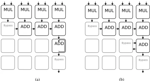
A possible implementation of a FIR filter on a CGRA would be to compute a tap on each PE on the first row and add the results on the row beneath it. Chaining the results together as shown in figure 3.3a would produce a result on the last PE on this row.

(27)

3.1 Filtering 11

Figure 3.2: Example FIR architecture for hardware implementations.

it would be accessed by several PEs. This memory would have to provide many ports or have several instances of the same values in different memory blocks. The same results can be achieved by retrieving the coefficients from the inputs at the same time as input data.

MUL Bypass MUL ADD MUL ADD MUL ADD ADD Bypass (a) MUL Bypass MUL ADD MUL ADD MUL ADD ADD Bypass (b)

Figure 3.3: Mapping of FIR filter on a 4x4 CGRA at 4 taps per clock with(a) and without(b) internal storage.

If the PEs don’t have the option of performing accumulative operations the results of this PE would have to be added together by using several PEs to accumulate the values as shown in figure 3.4b.

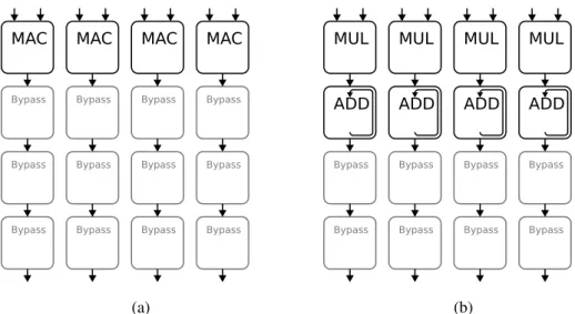
If the PEs had the option of performing multiply and accumulate (MAC) operations, the first row could perform this function and the final addition of the accumulated values would be calcu-lated by the rows below them as shown in figure 3.5a.

Another implementation would be to compute the same tap for several output samples on each clock. In this implementation each column would compute a different output sample over more cycles while performing the same number of taps overall. This approach allows for the use of a single port Register File for the coefficients as each column would use the same coefficient on each clock cycle. Once again the option of using accumulative operations allows the CGRA to output the final values. Using MAC operations only one row would be required.

(28)

12 Use case analysis MUL Bypass MUL ADD MUL ADD MUL ADD ADD Bypass (a) MUL Bypass MUL ADD MUL ADD Bypass MUL ADD ADD Bypass (b)

Figure 3.4: Mapping of FIR filter on a 4x4 CGRA at 4 taps per clock with(a) and without(b) acumulative operations.

Lastly, the control of which samples and coefficient to fetch from memory is a different task and would most likely benefit from a hardware solution within the memory controller for the accelerator. This module would receive the addresses of the samples and the coefficients to fetch and supply the CGRA with the right data by using its internal counter to emulate a circular memory block. This controller could also be responsible for correctly placing the results in memory.

3.1.2 Median filters

Median filters are very useful for removing noise in this type of signal. These are specifically useful for removing baseline wander by using the result of a large median filter as the baseline of the original signal [16]. The way a median filter works, is by calculating the median within a window around the sample as exemplified in figure 3.1c.

A simple implementation would be to have a section of memory the size of the window and for each sample, replace the oldest sample with the newest and calculate the median based on that set. The knowledge of the previous order can be used to simplify the process of reordering the modified set. Thus, by maintaining the order in both time and magnitude, the process is simpler and less computationally intensive.

This is an example of the type of task that would be ill suited for implementing on a CGRA. This algorithm heavily utilizes comparisons and control flow. To map this type of filter on a CGRA would require PEs with internal state and memory, effectively becoming small processors themselves. Thus not taking advantage of the parallelism the CGRA accelerator would provide and would most likely be faster and more cost efficient to perform this filter on the host CPU while the CGRA performs a different task.

(29)

3.2 Signal manipulation 13 MAC Bypass Bypass Bypass MAC Bypass Bypass Bypass MAC Bypass Bypass Bypass MAC Bypass Bypass Bypass (a) MUL ADD Bypass Bypass MUL ADD Bypass Bypass MUL ADD Bypass Bypass MUL ADD Bypass Bypass (b)

Figure 3.5: Mapping of FIR filter on a 4x4 CGRA at 4 output samples each with 1 tap per clock with (a) and without MAC operations (b)

3.2 Signal manipulation

In this application domain we commonly find applications that take advantage of signal manipu-lations such as subtracting a constant from each element of a vector to normalize it. This type of operation is reasonably trivial to map to a CGRA as the data-flow is constant. For example the figure 3.6 shows the mapping of subtracting a constant, applying a constant gain and adding the constant back. This example is simple but can be used to amplify a signal without affecting its mean value. SUB MUL ADD Bypass SUB MUL ADD Bypass SUB MUL ADD Bypass SUB MUL ADD Bypass

Figure 3.6: Mapping of an example application which can be used to amplify a signal without affecting its mean value.

Other commonly used signal manipulation algorithms are up-sampling and down-sampling. These would change the number of samples of a signal. In the case of down-sampling or

(30)

decima-14 Use case analysis

tion the typical implementation is to pass the original signal through a low pass filter and keep or discard samples according to the decimation factor. In the case of up-sampling or interpolation one would typically insert additional samples with a zero value in between each original sample and then pass the signal through a low pass filter with a gain equal to the up-sampling ratio as shown in 3.7. 0 20 40 60 80 100 120 140 160 180 200 -10 0 10 Input signal 0 100 200 300 400 500 600 -10 0

10 Input signal with padding (two 0s beween each sample)

0 100 200 300 400 500 600

-10 0

10 Interpolated signal (x3)

Figure 3.7: Example of x3 up-sampling using a 16 tap FIR filter

An example of an application where decimation is important is described in [18] where the EEG signals from 46 channels must be condensed to fit the inputs of a convolutional neural net-work.

These algorithms can be easily implemented on a CGRA by using FIR filters as proposed in the section 3.1. For implementing down-sampling one could modify the position of the taps and then only compute the FIR for samples we intend to keep, thus reducing the computational cost by the decimation factor. For implementing up-sampling one could perform the gain by applying the gain to the coefficients directly. Additionally the knowledge of which samples where "inserted" can be used to only compute the taps that correspond to the original samples. For example if the up-sampling had a factor of 2, the controller could alternate between feeding only the odd taps and then only the even ones, effectively "inserting" the new samples with no additional computation.

This approach to up and down sampling, replaces the execution time with controller complex-ity. This is an aspect of accelerator design and trade-off analysis that is heavily dependent on the application. As an example, the execution time in this task is at least halved by having a slightly more complex controller. However this does require that the controller design accounts for this type of optimization. In this case, the technique the controller enables is simple and periodic, corresponding to simple changes to the addresses. More complex optimizations such as ordering butterflies by twiddle factor in FFT execution are substantially more complex.

(31)

3.3 Signal transformation 15

3.3 Signal transformation

Signal transformations are very common in this type of application. In this study we will be fo-cusing on Fast Fourier Transform (FFT) for transforming signals from the time domain to the frequency domain. Other more esoteric transformations can be useful, however, none are as com-mon as in this domain as FFT/DFT.

3.3.1 Fast Fourier Transform

The research shown in [21] utilizes FFT based features to classify sleep states based on EEG signals. The resulting features correspond to the sum of the absolute power in a frequency band. The results are then divided by the sum of these features to provide relative values. The frequency band is divided into delta (0.5-4Hz), theta (4-8Hz), alpha (8-13Hz), beta (13-20Hz) and gamma (20-64Hz).

The most common algorithm for computing DFT would be Cooley–Tukey FFT algorithm due to the complexity of the computation being NLog(N). This FFT algorithm is based on exploiting some symmetry within the complex exponential to transform one FFT into 2 FFTs of half the size. The Discreet Fourier Transform (DFT) is calculated by computing the correlation between the signal and the sine and cosine at each frequency as in 3.1.

X[k] = N−1

∑

n=0 x[n]WNnk (3.1) where WN = e− i2π

N corresponding to the Euler representation of complex sinusoidal signal. By

separating the odd and even elements we can express the result of a N point DFT based on the results of 2 N/2 point DFTs. X[k] = N/2−1

∑

r=0 x[2r]WN2rk+ N/2−1

∑

r=0 x[2r + 1]W_N(2r+1)k (3.2)

We can pull WNk out of the sum and by noting that WN2= e −i2π N/2 _{= W} N/2we reach equation 3.3. X[k] = N/2−1

∑

r=0 x[2r]W_N/2rk +WNk N/2−1

∑

r=0 x[2r + 1]W_N/2rk (3.3) X[k] = Xeven[k] +WNkXodd[k] (3.4)

The expression 3.4 leads to what is commonly called a butterfly as each 2 inputs are added to the other and multiplied by a complex coefficient. These coefficients are commonly called twiddle factors and would always have a magnitude of 1 and would be the same for each output index k. Additionally the coefficients are symmetric and allow us to only compute a single complex multiply and either add or subtract the result for each butterfly as shown in figure 3.8. This process

(32)

16 Use case analysis

of splitting a large FFT into 2 smaller ones can be repeated until N is 1 in which case the X[k] = x[t]. -1 -1 -1 -1 -1 -1 -1 -1 -1 -1 -1 -1 -1 -1 -1 -1 -1 x[0] x[4] x[2] x[6] x[1] x[5] x[3] x[7] X[0] X[1] X[2] X[3] X[4] X[5] X[6] X[7] W_N0 W_N1 W_N2 W_N3 W_N0 W_N2 W_N0 W_N2 W_N0 W_N0 W_N0 W_N0

Figure 3.8: Dataflow of a 8 point FFT butterfly

This type of implantation has the disadvantage that N should be a power of 2. The solution to performing FFT with a N which is not prime is to divide it into many smaller FFTs based on the factors of N as detailed in [22].

To implement this on a CGRA accelerator one would ideally want to map a full Butterfly to the CGRA. The implementation of a generic butterfly would require a complex product, a complex addition and a complex subtraction.

The most obvious approach would be to add support for complex operations, however, the size of the data paths within the CGRA would have to double. This approach would be viable in circumstances where FFT or other algorithms based on complex numbers constitute the majority of the operations. Alternatively, executing these complex operations on integer based hardware would consume more CGRA resources. The complex addition and subtraction can easily be split into 2 integer additions or subtractions. The part of the butterfly operation that would require these operations can be mapped to CGRA if it has diagonal connections as in figure 3.10. Mapping a complex multiply is significantly harder, requiring more capabilities from the CGRAs intercon-nections or elements. If the CGRA has 2 inputs per PE in the first row the CGRA can execute a full complex multiply per clock if it has some diagonal connections as in figure 3.9.

Unfortunately this requires that several inputs receive the same data which implies a more complex management of information. To include the rest of the butterfly operation would require other data inputs.

A different approach would be to pre-load the complex coefficient in the PE that would use it. This solution could result in the mapping shown in figure 3.10. This not only requires diagonal connections but also some 2 hop connections or additional input ports. Due to the differences in the data paths of this solution, S1 has to be delayed one clock cycle in relation to S2.

In the first set of butterfly operations the coefficients are always 1 or -1 allowing us to skip the complex multiply entirely. If the source data only has a real component, the implementation of

(33)

3.4 Feature extraction 17

MUL

Bypass

MUL

ADD

Bypass Bypass

MUL

ADD

Bypass

MUL

Figure 3.9: Mapping of a complete complex multiply.

the first layer of butterflies can be simplified further, allowing for a butterfly operation for every 2 columns as in figure 3.11.

The optimal execution order for this type of approach would be to perform the first layer with this doubly fast version and switch to the solution proposed above in which the butterfly operation with the same twiddle factor are executed consecutively.

3.4 Feature extraction

Feature extraction is in itself a very broad field dedicated to producing valuable metrics for un-derstanding the subject’s condition which can have wildly different complexities. Some of these features can be as simple as the peak value within a vector, while other features would require complex machine learning algorithms to detect patterns in EEG signals [18, 21, 23].

In the interest of determining the computational requirements of this type of algorithms, we consider:

• Examples of low complexity such as the extraction of statistical metrics from the time be-tween heartbeats for ECG signal analysis.

• Examples of medium complexity such as reliably identification of the R peak on ECG sig-nals.

• Examples of high complexity such as utilizing a pre-trained convolutional neural network to identify patterns in EEG signals.

The first obstacle we should consider is the separation between what part of the algorithm can be mapped to the CGRA accelerator and the part which would benefit from being executed on the host CPU. An example of this is that calculating the peak value in a vector is trivial for a DSP but, would require the addition of comparator operations and support for control flow operation or state

(34)

18 Use case analysis Bypass

MUL

Bypass

ADD

Bypass

MUL

ADD

SUB

Bypass

MUL

ADD

Bypass

MUL

Bypass

SUB

Re(Tw) Im(Tw) Re(Tw) Im(Tw)

Re(S1) Re(S2) Im(S2) Im(S1)

Re(R1) Re(R2) Im(R1) Im(R2)

Figure 3.10: Mapping of a full FFT buterfly on a 4x4 CGRA where Tw represents the current twiddle factor, S1 and S2 represent the inbound samples and R1 and R2 represent the outbound samples

machines, to compute this task on a CGRA. On the other hand, calculating the mean square of a signal can be easily mapped to a CGRA and would compute it as a rate of 4 samples per clock.

The ideal separation would be to perform the loops with a fixed number of iterations and a known number of inputs and outputs on the CGRA and perform a sweep over the output vector using the host CPU if it is necessary.

The next obstacle to mapping certain feature extraction algorithms to a CGRA accelerator is the need for internal state. The type of applications in which CGRAs excel are one that use it as a stateless pipeline. Using of internal state or conditional execution is a less effective use of a CGRA architecture. However there are several solutions to this kind of problem. One such solution is to add to each PE a finite state machine that changes its operation. This solution would however increase the area and energy consumption of the PEs bringing them closer to small compute cores in both complexity and versatility.

Another way to add some control flow to the CGRA is to add comparators and allow the com-parison to affect the data, for example use a product to gate the values of a data path. Effectively one could map an algorithm such that both options are computed as well as the condition, and use the condition to gate the values setting them to 0 if the value is to be ignored and finally the results are added.

Alternatively one could use non linear operations such as the ReLU operation (which is a linear rectifier that outputs 0 if the input is negative). For example, calculating the peak value within a vector could be done by accumulating only the positive results of the subtraction between the input

(35)

3.4 Feature extraction 19 Bypass

ADD

Bypass Bypass Bypass

SUB

ADD

SUB

Bypass Bypass

Figure 3.11: Mapping of the first layer of FFT where the twiddle factors are 1 and -1

and the current maximum. This would transform a condition based loop into a purely arithmetic loop that has an accumulated result. This approach to algorithms based on state is much simpler in the sense that it would only require the addition of simple operations to the PEs but may not always be viable due to the limited number of PEs in the array.

3.4.1 Signal transformation based feature extraction

Certain features, as discussed above, can be partially computed on the CGRA accelerator and partially on the CPU. In general, any set of element-wise operations could benefit from the CGRA accelerator. The same would apply to accumulative operations to the extent that within CGRA we can trivially calculate the sum of a vector as the vector is being produced.

As examples of this type of feature we can compute the mean of a vector and then subtract that mean from the vector while computing the sum of the square of the result. The root of the result is calculated on the host CPU to produce the standard deviation of the vector. While simultaneously starting to execute a different algorithm. Each of these operations are simple enough to utilize the entire bandwidth to the CGRA with minimal stall time in between tasks. If this series of operations were mapped to a 4x4 CGRA it could execute 4 samples per clock effectively taking dn/4e clock cycles to compute each set of vector operations.

3.4.2 Vector based feature extraction

More complex features require more layers of operations and are more computationally intensive. As an example, we shall consider the analysis of ECG signals to extract information about the QRS complex for each heartbeat, a very common task that is a particularly useful example as it is a very common and well explored area. The most common approach is based on Pan-Tompkins

(36)

algorithm [24] which uses several layers of signal transformations followed by a computationally simpler classification and validation.

In the Pan-Tompkins algorithm the first step is to pass the signal through a 5-15 Hz bandpass filter followed by a derivating filter. The result is then squared and averaged over a window of 0.15s. The result is a signal which can be used to find the QRS complex more easily than the original. The bandpass filter and derivating filter can be implemented as FIR filters. Squaring the signal is a simple enough task that it can be integrated into the mapping of a different component. The next steps of the Pan Tompkins algorithm are based on adaptive thresholds and physio-logical validation. These would preferably be executed on the host CPU.

In the research shown in [17] they use several features to distinguish between rest, walking and running. The features are calculated on 1.6s windows which overlap 50%. The mean, standard deviation, median, skewness, Kurtosis and Inter-quartile-range are calculated for each window.

The research shown in [21] utilizes several features to classify sleep states based on EEG signals. Among them are features such as the median of the absolute value for EMG or the correlation coefficient of the electrooculography (EOG) signals for the left and right eye.

This type of feature can be easily mapped to a CGRA as they are based on operations over a set of input data with little to no control flow. Other features such as calculating the entropy of a signal which involves producing a histogram of absolute values of the signal, are much harder to apply to a CGRA as they would require conditional operations and manipulation of memory addresses.

3.4.3 Neural network based feature extraction

Features produced as a result of a pre-trained neural network have the potential for very accurate parameters and can model nonlinear systems very well. The neural networks can be trained on very large data sets and produce systems that fit the great majority of subjects. However, if the results are poor for a particular individual, these systems could load a different neural network produced by further training the generalised version to fit the individual better.

In the context of low power biological signal processing, we can exclude training of the neural network as a valid use case for this accelerator. However, in cases where the nodes are linear, the process of calculating the derivatives of the network could be implemented in the CGRA. By also running a data set through a neural network and the accelerator one could run back-propagation algorithms on this type of low power system.

This process could potentially allow a small low power system that uses a CGRA accelerator to sporadically train its own network. For example a product could be pre-trained and then be "calibrated" to the user on first use.

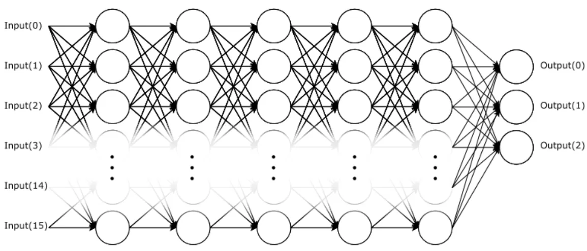
From the perspective of mapping a neural network to a CGRA, we can consider executing a neural network as a series of matrix operations. Let us first consider a simplified example, a neural network comprised of linear nodes with bias, with 5 layers, each 16 wide and with 3 output nodes as shown in figure 3.12. Computing the output value of a single node is effectively the same as

(37)

3.4 Feature extraction 21 Input(0) Input(1) Input(2) Input(3) Input(14) Input(15) Output(0) Output(1) Output(2)

Figure 3.12: Example Neural Network of size 16x5 with 3 outputs

the dot product of 2 vectors, where the first vector is the inputs and the second is the weights for each input. To add the bias we could add a 1 as an additional element of the first vector and add the bias as the additional element of the second. This process can be easily executed on a CGRA, simply by configuring it to calculate the dot product of 2 vectors and looping over each node on each layer.

A more generalised view of neural networks would be to separate the neuron from its activation function. In the example above the output of each neuron is a linear combination of the inputs with a bias, although, other types of neural networks can support many different non-linear neurons. The same also applies to the activation function. In the example above the activation function is linear, however, it is very common to use nonlinear activation functions. In particular the sigmoid activation function is commonly used to limit output values of the neurons, turning an unbounded scalar into a measure of the "activation" of the neuron ranging form 0 to 1, as shown in image 3.13c. Unfortunately this function is based on an exponential and therefore is very hard to compute on a CGRA.

Relu Sigmoid SoftMax

1 0 1 1 0 1 0 2.5 10.2 16 -1.9 0.9 2.4 -0.9 0.1 0.9 2.6 -0.8 0 0.997 16 0.003 0 0 0 0 0 0 0 0 0

(38)

Another common activation function is a linear rectifier where the negative outputs are re-placed with 0. The most common notation is to add a layer of Rectified Linear Units (ReLU). The use of ReLUs allows for some non linear behaviour while still using linear neurons and with-out changing the derivatives of the training algorithms. As a result, the same back-propagation techniques can be applied, and from the perspective of the derivative calculations ReLU layers are linear.

Convolutional neural networks are a different form of neural network based on restricting the inputs of each node to a subset of the inputs. This focuses the output of each node on a section of the input data thus allowing for more nodes within the same overall computation time. The inputs each node has access to are in general in relation to a position, for example each node could correspond to a pixel of an image and the output is based on a small region around each original pixel. In this case, the input is a biological signal, as such we would want to map the inputs temporally, an example of this is shown in subsection 3.5.

When applied to this domain the type of neural network in use would also be chosen with the system’s constraints in mind. As such, for the purposes of feature extraction on this type of system we would expect neural networks with linear neurons and activation functions of the complexity of ReLUs. Alternatively more complex neurons and activation functions can be added to the PEs to allow for neural networks of a smaller size. Convolutional layers would not be an issue. On the other hand, exponential or recursive layers would probably go beyond what a low power CGRA could provide.

3.5 Classification

Classification is once again a very diverse category. The simpler categorization algorithms such as checking a series of boundaries or thresholds would not benefit from CGRA acceleration. Ap-plications like [23] which aims to detect heart arrhythmia based on ECG signals, determine the state based on a series of thresholds. Some applications use decision trees as classifiers, like the one used in [17] where 30 features are used to classify between rest, walking and running. These applications rely on normalized features with high reliability, which is not necessarily the case and would require additional classifiers to discard invalid results.

Using linear discriminants as discussed in [16] could provide the set of thresholds that a pro-duction application would then use as a fixed classifier. Implementing this type of classification would involve multiplying each vector of features with the right transformation matrix and finally passing the result through a series of comparisons. If the number of features or the number of clas-sifications is large it might be worthwhile to use the CGRA to apply the transformation matrix.

Applications with more extreme classifiers use neural networks to perform the classification. These neural networks would have the same constraints and requirements as the neural networks described in section 3.4.3 for feature extraction with the exception of activation function of the output nodes.

(39)

3.5 Classification 23

In the domain of neural networks for feature extraction, the output values would most likely be scalar, however, for classification the output values would ideally be boolean. A very common activation function for output nodes is SoftMax, where the exponential of the value of each output is divided by the sum of the exponential of each output value to produce boolean like values ranging from 0 to 1. The distance to a 0 or 1 can be viewed as a measure of the uncertainty of the answer. For example a neural network that distinguishes between different people would ideally have a single output as 1 and the others would be zero. However, a result that produces .8 for a 1 and .2 for a 2 would still categorize as a 1 but could also show the uncertainty of the output in a situation where the distinction is less apparent.

The research described in [25] uses a large neural network to classify what type of image the subject is seeing based on EEG signals. The neural network in use is comprised of 10 layers of linear neurons with ReLU layers in between. The width of the network is 3200 to receive a batch of sample data at a time. Each batch consists of a 0.2s clip of 64 channel 250Hz EEG recordings. There are 5 SoftMax output nodes, one for each category – faces, places, objects, scrambled faces, and scrambled places.

The authors of [18] use a convolutional neural network on filtered EEG signals to categorise the motion of a subject. The resulting convolutional neural network distinguishes between clench-ing of the left or right hand with 81% classification accuracy. The convolutional neural network used to achieve this takes a 46 x 46 pixel image and is comprised of 2 convolutional layers, 2 max pooling layers, a fully connected one and 2 output nodes. The pooling layers can be implemented on the CGRA by using addition, subtraction and the ReLU operation as shown in figure 3.14. The neural network takes a 46 x 46 pixel image as an input, which corresponds to the data from the 46 channels. The first convolutional layer had 40 kernels of size 5x5, each producing a 22x22 image which is pooled to 11x11 image by a max pooling layer. The second convolutional layer had 100 kernels of size 5x5, each producing a 7x7 image which is pooled to 3x3 image by a max pooling layer. The last fully connected layer has 500 neurons whose results are then used by the output nodes.

As an example, we can check whether this algorithm is feasible for a small form factor system to compute. If the inputs are EEG signals in 46 channels at 250 Hz, they can be filtered using the FIR filters proposed in section 3.1.1 and decimated as explained in section 3.2 to produce the 46x46 input array which would correspond to a 400 ms window. Computing the first layer corresponds to 40x22x22 vector products of size 25, and similarly the second layer corresponds 100x7x7 vector products of the same size. If we consider a 5x5 CGRA which can pipeline a 25 wide vector product in 5 clock cycles, then the CGRA would take 40x22x22x5 = 96800 clock cycles to compute the first convolutional layer. The max pooling layer can be implemented using the same approach as shown in 3.14 which would alow a 5x5 CGRA to compute the max pooling layers at the rate of 2 values per clock cycle. The first pooling layer would take 40x22x22/2 = 9680 to compute. Similarly the second convolutional layer would take 100x7x7x5 = 24500 clock cycles and the second pooling layer would take 100x7x7/2 = 2450 clock cycles. The fully connected

(40)

24 Use case analysis Bypass ADD Bypass Bypass SUB ReLU Bypass ADD Bypass Bypass SUB ReLU

Figure 3.14: Maximum of two numbers using ReLU, two sets at a time on a 4x4 CGRA

layer would correspond to 500 vector products of size 900 which could take 90000 clock cycles. Totaling 223430 clock cycles plus the initial filtering and the down sampling layers, if the CGRA ran at 100MHz this would take at least 2.2ms to compute. Based on this estimate we can say that this type of algorithm could be executed on the CGRA. The unfortunate disadvantage of this algorithm is the memory requirements of this task, as it has a large number of coefficients and intermediate values that must be stored and supplied to the CGRA for each layer of the NN.

3.6 Selected use cases

In the interest of validating and testing the accelerator architectures studied in this dissertation we will be considering the following 3 use cases.

The first use case to be implemented on the CGRA is an ECG based arrhythmia detection platform. That would provide 24h ambulatory ECG monitoring, as it is becoming more and more important in both homecare and clinical settings to prevent cardiovascular disease [17]. Usually, patients have to carry a bulky instrument for continuous ECG monitoring, which restricts their mobility and makes them uncomfortable with so many electrodes and cables around their bodies. There is a growing demand for small-size, compact wearable ECG acquisition systems [17].

This would require filtering of the inbound ECG data, followed by extraction of several fea-tures of each heartbeat, leading to the classification algorithms shown in [23] that distinguishes between different states of arrhythmia and a normal heartbeat. Once a state of arrhythmia is detected other metrics such as heart rate variability can be computed and stored or transmitted. Among these metrics would be LF (low frequency between 0.04 - 0.15 Hz) and HF (high fre-quency between 0.15-0.4 Hz) which require FFT results.

The second use case is based on the work conducted at Instituto de Engenharia de Sistemas e Computadores, Tecnologia e Ciência (INESC TEC) which aims to identify an individual based on

(41)

3.6 Selected use cases 25

their ECG. The system these researchers have developed is based on extraction of several features of each heartbeat which are normalized and validated before being introduced in the classifier. The classifier that distinguishes between different individuals is based on a pre-trained machine learning algorithm.

The third use case is based on the research described in [18] in which a neural network is used to identify clenching of the left or right hand based on EEG signals. This would require filtering and down sampling of 46 channels of EEG signals followed by a classifier based on a convolutional neural network. The classifier described in section 3.5 represents the task of sporadically executing a large classification task in a production setting. The goal would be to study the application of a task of this complexity to a low power CGRA architecture, thus the focus is on executing a neural network with the correct size regardless of the coefficients themselves. This specific use case has the advantage that the data set used in [18] is publicly available, as such, it would be possible to demonstrate an accelerator architecture with real data and replicate their results.

(42)

(43)

Chapter 4

Architecture analysis

This chapter is dedicated to the architectural and design choices involved in implementing a CGRA to be used in low power systems for processing biological signals. The implications of these constraints are very complex. The CGRA element as described in chapter 2 has been thoroughly explored and as such we have many avenues to explore based on the solutions others have reached when designing systems for other domains. The biological signal processing aspect to this study as explored in chapter 3 presents many requirements and limitations to any architecture designed for this domain. Furthermore designing an architecture when the energy consumption is such a relevant factor, presents its own limitations to any potential solution. In this chapter we will consider:

• The height and width of the CGRA and consequently the number of processing elements. • The bit-width the PEs support.

• The method for handling and loading configurations to the PEs. • The method for handling and loading internal data storage. • Heterogeneous functionality of PEs throughout the CGRA. • Different approaches to the controller for the CGRA.

In the interest of clarity we will assume that the direction of the flow of data would be from top to bottom, that the PEs into which data is loaded are at the top of the array and that the result would be retrieved from the bottom row of the array. This would allow us to think of the flow of data and the execution of operations in the same way as a data flow graph or the snip-it of code the task would correspond to. The implications of this assumption are not significant as the CGRA can be rotated or flipped to comply with any direction we would need.

4.1 Height and width of the CGRA

The height and width of the CGRA is the most discernible design decision, and one would be inclined to think that a larger CGRA is always the solution to an algorithm that cannot be mapped (whose datapath would not fit within it). The obvious contradiction to this notion is any algorithm that includes feedback. Excluding tasks with internal feedback loops, most tasks can be unwrapped

(44)

28 Architecture analysis

and pipelined. This process generally consists in separating the task into small elements displaced in time such that, at any moment each element is performing a step of an iteration, while simul-taneously its neighbours perform their corresponding step of a previous or subsequent iteration. The resulting data flow would have a maximum length that in this context translates into the num-ber of PEs that connect an input to an output, and also a maximum width which is associated to a maximum amount of data that has to flow through the pipeline. With these considerations in mind we would want a CGRA that is very tall to accommodate any algorithms whose data path is very long. Similarly we would want a CGRA that is very wide as to accommodate any algorithms whose datapath includes lots of intermediate values. However in this case, the energy consump-tion is a heavy factor and any unused PEs constitute sources of unnecessary static power loss. One way to evade this static loss is to power gate sections of the array.

Figure 4.1: Figure to illustrate the relationship between static and dynamic power in a 4x4 24-bit CGRA (based on the activation values of a 4-tap FIR filtering ECG data)

Figure 4.2: Graph of resource utilization for sizes between 2x2 and 8x8 based on FPGA imple-mentations

As shown in figure 4.1 the static power loss is significant. In a sense, we would want a small CGRA that could map the applications we would need while power gating unused sections for less resource intensive algorithms.

Configurable coarse-grained array architecture for processing of biological signals

F

E

U

P

Configurable coarse-grained arrays

architecture for biological signal

processing

João Pedro Sauvarin Lopes

M

Resumo

Abstract

Acknowledgements

Contents

List of Figures

List of Tables

Abbreviations

Chapter 1

Introduction

1.1

Context

1.2

Motivation

1.3

High level objectives of the document

1.4

Structure of the document

Chapter 2

Study of relevant literature and

published research

2.1

Processing biological signals

2.2

Coarse grained reconfigurable arrays

PE

PE

PE

PE

PE

PE

PE

PE

PE

PE

PE

PE

PE

PE

PE

PE

2.3

Applications of CGRAs

2.4

CGRAs in low-power biological signal processing

2.5

Summary

Chapter 3

Use case analysis

3.1

Filtering

3.2

Signal manipulation

3.3

Signal transformation

∑

∑

∑

∑

∑

MUL

MUL

ADD

MUL

ADD

MUL

3.4

Feature extraction

MUL

ADD

MUL