Contributions on Deep Transfer Learning

(1)

F

ACULDADE DE

E

NGENHARIA DA

U

NIVERSIDADE DO

P

ORTO

Contributions on Deep Transfer

Learning

Chetak Kandaswamy

MAP-tele Doctoral Program in Telecommunications Supervisor: Jaime dos Santos Cardoso (PhD) Co-supervisor: Luís Miguel Almeida da Silva (PhD)

(2)

(3)

Contributions on Deep Transfer Learning

Chetak Kandaswamy

MAP-tele Doctoral Program in Telecommunications

(4)

(5)

i

Abstract

Machine Learning (ML) is reshaping our world by building machines that can see, read, listen, talk, and write (Marr, 2015). For example, imagine you want to eat your favorite food and ask a mobile app what are the nearby restaurants that serve your favorite food. The app uses a ML algorithm to analyze the information of your location and time to provide better service. Imagine a startup that wants to use ML algorithm optimize their resources and requirements. Envision a scenario where a breast cancer patient and a surgeon want to plan a surgery. Generally, it takes a highly trained surgeon’s subjective evaluation of the breast cancer surgery to make treatment decisions. Employing ML algorithms allows an objective evaluation of the surgery with a sense of femininity (aesthetic metric by (Beadle et al., 1984)), using 3D imaging that helps the patient and the doctor to visualize and collectively decide what they are seeing, and then make a informed decision about the surgery (Oliveira, 2013).

The ability of ML algorithms to automatically understand the contents of images opened new ways to tackle prominent computer vision challenges like view point variation, illumination, occlu-sion, scale, deformation, background clutter, and intra-class variation. Especially, Deep learning algorithms like Stacked Denoising Autoencoders, Convolutional Neural Networks, and Deep Be-lief Nets have addressed these challenges with state-of-the-art results and have surpassed human performance. The salient attribute of Deep learning algorithms is that they automatically learn fea-tures from a large number of data samples without overfitting the model. Deep learning provides a partial solution to the research statement how to get computer programs to self-learn patterns from data. We consider machine learning as a broadening field which integrates interdisciplinary knowledge of learning processes from other fields such as psychology, biology, neuroscience, and economy. From this we attempt to answer questions such as: what kind of process can lead to learning, under what conditions, and for what kind of data? (Mitchell, 2006) In this thesis we integrated knowledge of deep learning with transfer learning where the learning is inspired from human-like learning processes to build our Deep Transfer Learning framework:

“how to get computer programs to self-learn patterns in data-efficient and domain-general way?”

Our survey on the state-of-the-art machine learning methods that use self-learn patterns lead to deep learning models. The subsequent question is about how learning algorithms can be inspired from human-like learning processes. For the sake of simplicity, we narrowed our scope down to human like knowledge transfer from one scenario to another.

It is interesting to study the various possible cases of transfer learning settings based on the distributions, posterior probabilities, learning function and the classification tasks. We have de-signed three main mechanisms that harness the advantages of our proposed Deep Transfer Learn-ing (DTL) framework: 1) Layerwise Transfer LearnLearn-ing (LTL), 2) Source-Target-Source (STS) and 3) Deep Transfer Learning Ensemble. First, we developed two approaches based on LTL mecha-nism : a) Transfer Learning unsupervised (TLu) and b) Transfer Learning supervised (TLs). On

(6)

the other hand, STS mechanisms were tested for both single and multi-source problems. Finally, we developed DTLE as an ensemble of various LTL approaches. To analyze the effectiveness we assess the designed DTL framework for practical applications like drug discovery and cross-sensor biometric identification. We also implemented a DTL software based on an interactive interface for GPU based machine learning algorithms. This software provides an interface to baseline and various transfer learning methods.

(7)

iii

Resumo

Aprendizagem Computacional (AC) consiste na criação de máquinas capazes de ver, ler, ouvir, falar e escrever (Marr, 2015). Por exemplo, imaginando que desejamos comer o nosso prato fa-vorito e nos aconselhamos com uma aplicação móvel relativamente a restaurante próximos que sirvam tal prato, a aplicação utilizará um algoritmo de AC para analisar a informação relativa à localização do utilizador de modo a proporcionar o melhor serviço possível. No caso alternativo da criação de uma startup tentando cimentar o seu negócio, um algoritmo de AC facilitará o pro-cesso de como economizar recursos suficientes. Ainda num terceiro caso, num cenário em que um paciente de cancro da mama e um cirurgião querem planear uma cirurgia, as decisões são geralmente tomadas através de uma avaliação subjetiva levada a cabo por um cirurgião altamente especializado. A utilização de algoritmos de AC nesta aplicação específica introduziu um maior grau de objetividade (Beadle et al., 1984) através de informação de imagiologia 3D, ajudando tanto o médico como o paciente a atingir coletivamente uma decisão bem informada relativamente à cirurgia (Oliveira, 2013).

A capacidade de algoritmos de AC de automaticamente compreender o conteúdo de imagens abriu novas possibilidades de encarar desafios proeminentes de visão computacional, como vari-ações de ponto de vista, iluminação, oclusão, escala, deformação, variabilidade de background ou variação intra-classe. Em especial, algorithmos de aprendizagem profunda, como deep al-gorithims: Stacked Denoising Autoencoders, Convolutional Neural Networks ou Deep Belief Nets mostraram-se capazes de abordar estes desafios e apresentar performance ao nível do es-tado da arte, ultrapassando largamente o potencial humano para realizar tais tarefas. O atributo mais saliente relativo a algoritmos de aprendizagem profunda foca-se na sua capacidade de auto-maticamente aprenderem características a partir de uma grande quantidade de dados, sem causar overfitting dos modelos treinados. Aprendizagem profunda permite uma solução parcial à questão comum nesta área de investigação relativa a como conseguir que computadores sejam capazes de entender de forma autónoma padrões em grandes quantidades de dados. De modo a atingir este último desafio, a área de aprendizagem computacional tem alargado o seu espectro interdisci-plinar através da integração de conhecimentos de especialistas de outras áreas, como a psicologia, a biologia, as neurociências ou a economia, de modo a entender que processos humanos con-duzem à aprendizagem e integração de conhecimentos dada uma série de dados sob uma série de condições (Mitchell, 2006). Nesta tese, integrámos o conhecimento de aprendizagem computa-cional profunda com transfer learning, em que a aprendizagem é inspirada no processo humano de aprendizagem, para construir a nossa framework de Deep Transfer Learning:

“como conseguir que computadores sejam capazes de aprender, de forma autónoma, padrões de maneira eficiente em termos de dados, e para domínio generalizado?”

Na presente tese o foco de investigação recai sobre métodos de AC capazes de auto-aprenderem padrões através da utilização de métodos de aprendizagem profunda. A questão subsequente prende-se com como desenvolver tais metodologias de forma inspirada no processo de aquisição

(8)

de conhecimento do ser-humano. Como simplificação, reduzimos o espectro de interesse na trans-ferência de conhecimento entre duas tarefas de modo a utilizar conhecimento adquirido numa para resolver outra.

É interessante estudar uma série de possíveis variações no processo de transferência de apren-dizagem, quer ao nível das distribuições, probabilidades posteriores, funções de aprendizagem e também tarefas de classificação. Foram criados três mecanismos base da framework de deep transfer learning: 1) Layerwise Transfer Learning (LTL), 2) Source-Target-Source (STS) e 3) Deep Transfer Learning Ensemble. Relativamente à primeira metodologia, duas abordagens foram tomadas: a) Transferência de conhecimento não-supervisionada (TLu) e b) Transferência de con-hecimento supervisionada (TLs). Por outro lado, os mecanismos de STS desenvolvidos foram tes-tados tanto em problemas com uma fonte de informação como em problemas de múltiplas fontes. Finalmente, foram também desenvolvidas e testadas metodologias ensemble de várias abordagens LTL. De modo a analisar a eficácia dos métodos desenvolvidos, testes práticos foram levados a cabo ao nível de descoberta de fármacos e também de biometria inter-sensor. Um software de DTL baseado em interface interativa para algoritmos de AC baseados em GPU foi também imple-mentado. Este software fornece uma interface para problemas baseline e outras metodologias de transferência de conhecimento.

(9)

To my mother and father, to whom I owe everything.

To my sister and my brother, for being driving force in my life.

(10)

(11)

vii

Acknowledgments

I would like to express my sincere gratitude to my advisor Professor Jaime dos Santos Cardoso for the continuous support of my PhD study and research, for his patience, motivation, enthusiasm and immense knowledge. The joy and enthusiasm he has for his research was contagious and motivational for me, even during tough times in the PhD pursuit. I am also thankful for the excellent example he has provided me as a successful researcher and Professor. I could not imagine having a better advisor and mentor for my PhD study.

Furthermore, I am very grateful to my co-advisor Professor Luís Miguel Almeida da Silva, for the opportunity to develop my PhD study in the area of deep learning, for the insightful comments both in my work and in this thesis, for her support and for many motivating discussions. I appre-ciate all his contributions of time, ideas, and funding to make my PhD experience productive and stimulating. His guidance helped me in all the time of research and writing of this thesis.

I extend my gratitude to NNIG (Neural Network Interest Group), INEB for all the conditions provided. I am very glad to have had the possibility of being embraced by this group. I am especially gra teful to: Luís. A. Alexandre, Jorge. M. Santos and Joaquim Marques de Sá. A very special word of gratitude is due to Ricardo Sousa, Tiago Esteves and Telmo Amaral, for their constant support and encouragement.

I extend my sincere thank to INESC Porto, for all the work conditions, infrastructure and technical support given to my PhD thesis and for the other challenges I worked in. I am especially grateful to all the members of the Visual Computing and Machine Intelligence (VCMI) group have contributed immensely to my personal and professional time. I am especially grateful to: Ana Rebelo, Ines Domingues, A. Filipa Sequeira, Samaneh Khoshrou, Eduardo Marques, João. C. Monteiro, João. P. Monteiro, Hooshiar Zolfagharnasab, Kelwin Fernandes and Helder Olivera. The group has been a source of friendship as well as motivation and collaboration. I thank FEUP for providing the support and conducive environment for my PhD. I would like to than Jonathan Barber for his support for building tools for the research work.

I shall also dedicate a few words to someone whose influence in my life spanned out the time I was his student from the degree to become a researcher. The way I reason about Mathematics, Science, Knowledge and Life itself was deeply influenced by the many things he taught me about. Thank you Professor Girish M Chandra.

I thank Professor Manuel Alberto Pereira Ricardo and Professor Rui Campos who are source of inspiration and provided me the guidance for building my research capabilities. I also like to thank Professor Adriano Moreira for believing in my professional ability and provided me the opportunity to pursue my PhD.

I thank Professor Helmut Prendinger for the opportunity to work in his lab on drones at Tokyo. I thank Andrew Holliday, Danielle Delatte, Johannes Laurmaa, Kim Samba, Pierre Ecarlat, Ragevendra Jain, Ruben Geraldas and Naoki Tada for their support during the research at National Institute of Information, Tokyo.

(12)

A special word of thanks to my friends without whose encouragement and unconditional sup-port it would be a challenge: Saravanan Kandasamy, Kumaresa Vanji, Abhishek Chatterjee, Bala-murugan Varadharajan, Herlina Jayadianti and Merle Planten. I would like to thank my Portuguese Professor Magarida Mouta who helped me to get along with culture shock and enjoy the interac-tion with beautiful land of Portugal. Thank you for your support when I have needed it the most.

For the ancestors who paved the path before me upon whose shoulders I stand. Kandaswamy family who have been my constant source inspiration, competition and encouragement. To my wife Jivitha Anand who became my source of encouragement and to my six months old baby Adya, you mean the world to me.

Thank you with all my heart! Chetak Kandaswamy

(13)

“Machine Learning is a core, transformative way by which we (academicians & industrial specialist) are rethinking how we’re doing everything”

Sundar Pichai

(14)

(15)

CONTENTS xi

List of Figures

2.1 Evolution of feature extraction methods from 1960’s to 2015. . . 10

2.2 Worldwide interest over time in the field of Machine Learning with Deep learning, Support Vector Machines and Random Forest. Keyword usage trends from 2004 to present. . . 12

2.3 Left: A regular 3-layer Neural Network. Right: A CNN arranges its neurons in three dimensions (width, height, depth), as visualized in one of the layers. Every layer of a CNN transforms the 3D input volume to a 3D output volume of neuron activations. In this example, the red input layer holds the image, so its width and height would be the dimensions of the image, and the depth would be three (Red, Green, Blue channels) (Li and Karpathy, 2015). . . 13

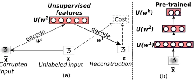
3.1 (a) Pre-training the first layer feature set, (b) Pre-trained K − 1 layers . . . 24

3.2 Samples from character recognition tasks . . . 28

3.3 Samples from various shape recognition tasks . . . 29

4.1 Transfer learning unsupervised (TLu) . . . 32

4.2 TLs for “L1” feature transference approach. . . 33

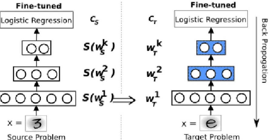
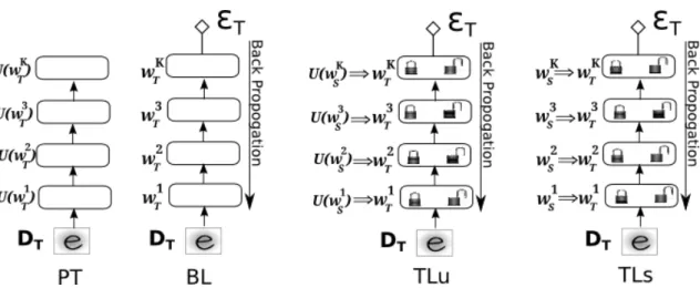
4.3 A pictorial representation of approaches: Pre-training (PT), Baseline (BL), Transfer Learn-ing unsupervised (TLu) and Transfer LearnLearn-ing supervised (TLs) with the option of lock or unlockfor each layer . . . 35

4.4 A pictorial representation of labels are different TL setting YS6= YT and PS(X ) 6= PT(X ) as the Jensen-Shannon divergence (JSD) between the source and the target distribution is greater than 0.8 . . . 38

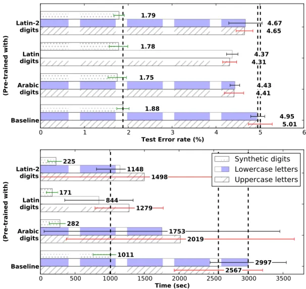
4.5 Comparison between TLu and baseline (dotted vertical line) for hard transfer prob-lems. Top: Average test error rate (%) (ε) on Synthetic digits, Lowercase and Uppercase letters datasets by reusing unsupervised features either from Arabic or Latinor Latin-2 dataset. Bottom: Computational time for the same experiments, in seconds. Box whiskers are standard deviations. . . 45

4.6 Comparison between TLu and baseline (dotted vertical line) for reverse transfer problems. Top: Average test error rate (%) (ε) on Arabic, Latin and Latin-2 datasets by reusing unsupervised features either from Synthetic digits or Low-ercase or Uppercase letters dataset. Bottom: Computational time for the same experiments, in seconds. Box whiskers are standard deviations. . . 46

4.7 Classification results on MAHDBase dataset (Arabic digits) for feature transfer-ence approach by reusing various layers, for different numbers N/c of training samples per class. Left: Average classification test error rate. Right: Average time taken for classification. . . 47

(20)

4.8 Classification results on MNIST dataset (Latin digits) for feature transference ap-proach by reusing various layers, for different numbers N/c of training samples per class. Left: Average classification test error rate. Right: Average time taken for classification. . . 47 5.1 (Left:) Relative improvement over baseline approach for character recognition tasks 3

& 4 as listed in Table 5.1; (Right:) Relative improvement for the tasks on the left, the regions are enclosed to observe relative improvement between two different approaches. We observe negative transference for TLs (supervised) approach as it gets stuck at local solution space of specialized features. TLu (unsupervised) approach easily recovers the fragile co-adapted neurons as the unsupervised features are not target specific. Also TLu improves over the baseline for complete training data. STS approach as intended shake the current local optimal solution, thus overcoming the specialized features of source network unlike TLs approach. The STS shows performance improvement, but unable to recover the fragile co-adapted neurons thus using complete target data, had lower performance than TLu and baseline. . . 53 5.2 Feature samples from first layer of non-canonical object recognition task. We observe the

transition of same features becoming more distinct, from BL towards STS approach are marked in red circle and from TLs towards STS marked in blue box. . . 53 6.1 A pictorial representation of Ensemble of Deep Transfer Learning. . . 57 7.1 A- Examples of different phenotypes (MOA) captured after compound incubation

of MFC7-wt cells. According to Ljosa et al. (Ljosa et al., 2013) only 6 of the 12 MOA were visually identifiable. B- Cell segmentation and feature extraction are performed using CellProfiler (Carpenter et al., 2006). For each cell, a variety of geometric, intensity, subcellular localization and texture features were extracted. . 67 7.2 Comparison of Baseline versus DTL approaches. Left: Baseline average accuracy

for classifying Pset1and DTL approaches for classifying Pset1reusing Pset2. Right:

Baseline average accuracy for classifying Pset2and DTL approaches for classifying

Pset2reusing Pset1. . . 71

7.3 Confusion matrices for the baseline and TL settings on the MOA problem (average outcomes over 10 repetitions). . . 72 8.1 Schematic representation of the GMM-UBM periocular recognition algorithm

pro-posed by Monteiro et al. (Monteiro and Cardoso, 2015). . . 77 8.2 Examples of images from each subset of the CSIP database. From (a-j)

respec-tively: AR0, AR1, BF0, BR0, BR1, CF0, CR0, CR1, DF0 and DR0. . . 79 8.3 Graphical representation of the MS-STS Rank-1 recognition rates obtained for all

the no-flash subsets of the CSIP database using all the flash datasets as sources, plotted against the respective BL, TLs and STS results. . . 88 8.4 Graphical representation of the MS-STS Rank-1 recognition rates obtained for all

the six possible orders of the chosen source datasets. Results concern to (a) AR0 and (b) CR0 as targets. . . 89 9.1 A pictorial representation of DTL soft user interface depicting the three DTL mechanisms 96 A.1 An illustrative picture showing a scenario in which smart drones build a shared

map and track the traffic movements at a freeway junction. Picture courtesy of NVIDIA. . . 101

(21)

LIST OF FIGURES xvii

A.2 Block diagram of model compression method for Ensemble of Deep Learning Models for Semantic Segmentation. . . 103 A.3 Block diagram of Extract-upscale method of Deep Learning Models modified for

Semantic Segmentation with skip connections. . . 104 A.4 Comparison between output labels for the single and compressed

FCN-ResNet-152 models, the ensemble and the ground-truth. In most cases, the compressed model is getting closer to the segmentation quality of the ensemble. . . 105 A.5 Screen shot of the Hikawa primary school premises marking the pool and the play

(22)

(23)

LIST OF TABLES xix

List of Tables

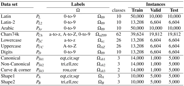
3.1 Number of instances available for each dataset. . . 28 4.1 Lists TLs, TLu Transfer Learning and Baseline Approach. An illustration of TLs

with all possible combinations for a 3 hidden layer network. . . 34 4.2 Average classification test error in percentage (ε) obtained with the baseline

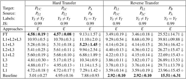
ap-proach along with the corresponding average training times (seconds) with GTX 770. . . 36 4.3 Changing the set of labels YS6= YT, YS= YT for arbitrary distributions PS(X ) 6=

PT(X ). Average classification test error (%) (ε) obtained for a target problem

using TLu approach for different combinations of: target data distribution (PT);

target label set (ΩT); source distribution (PS); source label set (ΩS) for Hard and

Reverse Transfer problems using SDA; The difference between distributions is given by Kullback-Leibler (KL) and Jensen-Shannon (JS) divergence. . . 39 4.4 Average Test Error (%) (ε) of TLs approaches for Hard and Reverse Transfer

problems using SDA . . . 40 4.5 Average Test Error (%) (ε) by reusing harder problem Latin-2 for classifying either

Lowercase or Uppercase letters. . . 42 4.6 Percent average classification test error (standard deviation) obtained for different

approaches, dataset, and numbers N/c of design samples per class for layer based, supervised feature transference for CNN model. . . 44 4.7 Percentage Average Error by reusing Latin at N/c = 1320 . . . 47 5.1 Comparison of percentage average error rate (ε) for BL, cBL, TLu, TLs and STS approach

for different ratios of target data (PT) reusing source (PS) distribution. Tasks 1 to 4 study

specificfeature transfer on character recognition problem and tasks 5 & 6 study generic feature transfer on object recognition problem. . . 54 5.2 Comparison of positive vs. negative transference using complete target data and

retrain-ing all layers; Performance is measured usretrain-ing percent average test error (ε) with 10 repe-titions; TLs shows positive transference for classifying MNIST PLreusing Lowercase PLC

same as Task 1. And negative transference for classifying PLCreusing PL, same as Task

3. In both cases iteratively repeating STS outperforms both BL and TLs approaches. . . 55 6.1 Percent average classification accuracy obtained for all three possible transfer

learning cases; 6 different experiments are performed on three different types of tasks i.e., character, object and biomedical image recognition; We compare estab-lished frameworks i.e., Baseline (BL), retrain specific DTL (DTLr), and transfer

specific DTL (DTLt) with our approach, retrain specific DTLE (DTLEr), transfer

specific DTLE (DTLEt), and Ensemble of DTL (DTLE); the difference between

(24)

7.1 Distribution of MOAs across batches for Pset1and Pset2with at least one common

batch between MOAs. Pset1and Pset2datasets have 6 mutually exclusive MOAs. . 68

7.2 Average accuracy in percentage and average computation time in minutes (stan-dard deviation in parenthesis) of the baseline (BL) and DTL approaches. The results are over 10 repetitions for the target data (PT) with compounds (C) and

source data (PS). . . 70

7.3 Comparison of accuracy obtained and total time taken per repetition in minutes with other state-of-the-art methods. . . 70 8.1 Technical details concerning the acquisitions setups used for each subset of the

CSIP database. . . 79 8.2 Rank-1 recognition rates, in %, observed for the GMM-UBM algorithm for all

possible cross-sensor scenarios in the CSIP database. . . 81 8.3 Rank-1 recognition rates, in %, observed for the SV-SDA algorithm for all possible

cross-sensor scenarios in the CSIP database. . . 82 8.4 Rank-1 recognition rates, in %, observed for the CNN algorithm for all possible

cross-sensor scenarios in the CSIP database. . . 82 8.5 Rank-1 recognition rates, in %, observed for the SDA methodology and the STS

approach. . . 84 8.6 Rank-1 recognition rates, in %, observed for the SV-SDA methodology and a

sin-gle cycle of the STS approach. . . 84 8.7 Rank-1 recognition rates, in %, observed for the CNN methodology and a single

cycle of the STS approach. . . 84 8.8 Rank-1 recognition rates, in %, observed for the CNN methodology and STS

ap-proach. . . 85 A.1 Comparison of Deep Learning object recognition architectures . . . 102 A.2 Model compression accuracy in Percentage with DTLE approach . . . 104 A.3 Model compression accuracy in Percentage with MS-STS approach . . . 105

(25)

LIST OF TABLES xxi

Acronym

BL Baseline

cBL Combined Baseline

CNN Convolutional Neural Network

conv Convolutional layer

CPA CellProfiler Analyst

CPU Central Processing Unit

CSIP Cross-sensor Iris and Periocular

dA denoising Autoencoder

DBN Deep Belief Nets

DNA Deoxyribonucleic acid

DNN Deep Neural Network

DTL Deep Transfer Learning

DTLE Deep Transfer Learning Ensemble

DTLEr Retrain Specific Deep Transfer Learning Ensemble DTLEt Transfer Specific Deep Transfer Learning Ensemble

FC Fully-connected layer

FCN Fully Convolutional Network

FT Finetune

GMM Gaussian Mixture Models

GPU Graphical Processing Unit

HCA High Content Analysis

HT Hard Transfer

IDSM individual specific models

JS Jensen-Shannon

(26)

KL Kullback-Leibler

LBP Local Binary Pattern

LOOCV Leave-One-Compound-Out Cross Validation

LR Logistic regression

LTL Layerwise Transfer Learning

MAP Maximum a Posterior

MCF7-wt Breast Cancer Expressing wild-type p53

MFCC Mel-frequency Cepstral Coefficients

ML Machine Learning

MOA Mechanisms of Action

MSCOCO Microsoft Common Object in Context

MS-STS Multi-source Source-Target-Source

NICE Noisy Iris Challenge Evaluation

NN Neural Network

pool Pooling layer

PT Pre-train

RBF Radial Basis Function

RBM Restricted Boltzmann Machines

RT Reverse Transfer

SAA Stacked Autoencoder

SDA Stacked Denoising Autoencoder

SGD Stochastic Gradient Descent

STS Source-Target-Source

SV Support Vector

SVM Support Vector Machines

TL Transfer Learning

TLs Transfer Learning supervised

TLu Transfer Learning unsupervised

UAV Unmanned Aerial Vehicle

UBM Universal Background Model

(27)

Part I

Introduction and Related work

(28)

(29)

Introduction 3

Chapter 1

Introduction

Machines have become an essential part of our everyday life. Towards the end of the last century, smart machines outperformed humans in mundane or highly specific tasks. These ma-chines use algorithms that are trained to automatically learn general laws from specific training data. Algorithms such as deep neural networks, support vector machines, Bayesian methods and many more have contributed to a wide range of applications including biomedical applications for drug discovery, data mining applications for detection of traffic signs, self-driving cars, biometric sensor interpretations, location identification of a person based on his wireless fidelity (WiFi) data, and aerial surveillance using swarm of unmanned aerial vehicles (UAVs). While these algorithms demonstrate the practical importance of machine learning methods, researchers are actively pur-suing more effective algorithms. Some of the interesting application of machine learning methods are now briefly discussed.

Computer Vision: Object recognition. The early success in hand-written digit recognition by convolutional (or time-delay) neural networks laid stepping stone for many computer vision applications. Semantic segmentation, object recognition, image recognition and 3D objects recog-nition in natural images are among the main examples.

Telecommunications: WiFi-Based Indoor Localization. An interesting problem faced by ubiquitous computing and social networking community is locating the smartphone user position in an indoor environment with WiFi data. This indoor WiFi localization problem is a challenge as it is very expensive to calibrate WiFi data for building localization models in a large-scale environ-ment. Moreover, it is known that the WiFi signal-strength values are function of time, device, and other dynamic factors. Machine learning algorithms are used to reduce the recalibration efforts by adapting to the dynamic changes in time and devices.

Biomedical Applications: Breast cancer drug discovery. Machine learning algorithms has paved a new way to better utilize the vast patients’ data for better and faster drug discovery and diagnosis of patients. Areas like early detection of Breast Cancer using Mammogramy Images and Magnetic Resonance Imaging of breast have benefited from such methods.

While these applications demonstrate the practical importance of machine learning methods, researchers are actively pursuing more effective algorithms.

(30)

1.1 Motivation

The world we live in requires knowledge of many things. We learn these things by continuously interacting with the external environment and developing skills accordingly.

We learn to play football for the fun of kicking the ball. Yet for playing football we require many other basic skills. To be a successful player, we use our previous knowledge of walking, running, jumping, kicking, etc. Our brain continuously learns to interact with the external envi-ronment and learns these specialized behavior patterns which may lead to winning. Inspired by this natural and continuous human learning, we attempt to train machines to mimic such human-like learning structures. The machine continuously learns and reuses its knowledge to solve different and specialised tasks, and this enables it to develop a wide knowledge base.

The world we live in presents both good and bad opportunities to learn. Football is fun to play, as long as we curb our habits which may prove to be counter productive. To be effective we should avoid playing without properly warming up first and look to leverage our strengths to positively affect the overall performance. The same is true even for machines. Training an algorithm with adverse knowledge produces negative performance on the intended task, and the resulting solution itself may falls into a local minima. It will be beneficial to utilize the adverse knowledge as a means and not as an end result.

1.2 Thesis Statement

The machine learning community in general has addressed challenges focused on the narrow view of the research question how to get computer programs to learn some class functions from ex-amples? To illustrate the limitation of this narrow view we do not have computer programs that have the ability to think like people. To break this view the community focused on Alan Turing’s ambitious research question: Can machines think? (Turing, 1950) which faced severe challenges on the definitions of machine and thinking. The question was later softened with Can machines do what we (as thinking entities) do? (Kurzweil, 2005). As a pragmatic option towards the goal of the General Intelligence paradigm, Tom Mitchell proposes a broader interdisciplinary view of machine learning involving computer programmers and statisticians who have already contributed to statistical-computational theories of learning processes. Together with other field experts like psychologist, economists, biologists and neuroscientists, they collectively questioned What kind of process can lead to learning under what conditions for what kind of data? (Mitchell, 2006).

This document attempts to address the fundamental question of how to get computer pro-grams to self-learn patterns from data. To this inquiry, we integrate interdisciplinary knowledge of human learning processes from other fields, for example: 1) psychological studies of the hu-man ability to easily adapt the learning from one situation to suit or adjust to another situation with minimal or no deviation (Perkins and Salomon, 1992), 2) neurological studies like the hu-man ability to perceive images with the hierarchical working structure of the neocortex (Hubel and Wiesel, 1959), and 3) other psychological studies of the human ability to continuously learn

(31)

1.3 Objectives 5

new processes (London and Sessa, 2007). In this thesis, we are interested in designing machine learning algorithms that are motivated by the above research question inspired from human-like learning processes.

1.3 Objectives

The main objective of this research is to develop a machine learning framework that attempts to self-learn the patterns and reuse extracted information from the data, enabling it to express the information as understandable by humans while making it possible to compete with state-of-the-art technology. In other words, the research aims to create an automated feature extractor that can be used to solve various tasks in spite of the tasks being different from each other. The core idea is to reuse the experience gained in learning to perform one or more tasks to help improve the learning performance of other tasks. Although, sharing or reusing the knowledge may lead to either an improved (positive) or degraded (negative) performance. In this work we intend to curtail negative learning or at least maintain the same performance as in the case of no sharing of knowledge.

In this sense, the self-learning feature extractor should produce generic and reusable features for multiple tasks from different domains. The performance of the designed framework is to be evaluated on various computer vision benchmark data as well as in two problem specific applica-tions: a biomedical application for drug discovery in breast cancer cells and sensor applications for person identification from multiple sensory data.

1.4 Contributions and Related Publications

A summary of the contributions of the thesis is as follows:

1. We have designed a Deep Transfer Learning (DTL) framework by combining the advantage of the hierarchical feature representation property of deep networks with the feature reuse property of Transfer Learning. This synergy led to the development of a self-learning feature extractor that produces generic and reusable features for solving multiple tasks. The DTL framework produced three mechanisms inspired by the human learning process that help to solve major challenges of machine learning problems:

(a) A layer-wise feature transference mechanism to reuse extracted features initially trained on a source domain and tested on a target domain with little modification of the model; this mechanism indeed enhanced the performance for many challenging computer vi-sion datasets, but is limited to reuse only features of source problems that lead to positive feature transference;

(b) A Source-Target-Source mechanism, where the layer-wise feature transference is op-timized by switching between multiple domains (both source and target) and thus ex-panding the optimal solution search space;

(32)

(c) A Deep Transfer Learning Ensemble mechanism where the layer-wise feature trans-ference mechanism is combined with the traditional ensemble learning.

2. We have investigated our designed layer-wise feature transference mechanism for applica-tion specific scenarios, such as the analysis of breast cancer cell images for drug discovery. 3. We extended our Source-Target-Source mechanism with a multi-source version for cross-sensor biometric classification applied to the identification of human anatomical structure in the periocular region.

Finally, we created a user interface for our DTL framework utilizing GPU parallel processing capabilities, which can be used by machine learning researchers to compare their methodologies and/or help in solving real problems in the field.

List of Publications arising from this thesis Journal papers:

• Kandaswamy, C., Silva, L.M., Alexandre, L.A., and Santos, J.M. "High-content Analysis of Breast Cancer using Single-Cell Deep Transfer Learning", Journal of Biomolecular Screen-ing, SAGE, January 8, 2016, doi: 10.1177/1087057115623451

• Kandaswamy, C., Monteiro, J.C., Silva, L.M and Cardoso, J.S. "Multi-source Deep Transfer Learning for Cross-sensor Biometrics." Neural Computing and Applications, 1-15, 2016, doi: 10.1007/s00521-016-2325-5

Conference papers:

• Kandaswamy, C., Silva, L. M., Alexandre, L. A., and Santos, J. M. Deep transfer learning ensemble for classification. In Advances in Computational Intelligence, pages 335–348. Springer, 2015a. doi: 10.1007/978-3-319-19258-1_29

• Kandaswamy, C., Silva, L. M., and Cardoso, J. S. Source-target-source classification using stacked denoising autoencoders. In Pattern Recognition and Image Analysis, pages 39–47. Springer, 2015b

• Kandaswamy, C., Silva, L. M., Alexandre, L. A., Sousa, R., Santos, J. M., de Sá, J. M., et al. Improving transfer learning accuracy by reusing stacked denoising autoencoders. In IEEE International Conference on Systems, Man and Cybernetics (SMC), pages 1380–1387. IEEE, 2014b. doi: 10.1109/SMC.2014.6974107

• Kandaswamy, C., Silva, L. M., Alexandre, L. A., Santos, J. M., and de Sá, J. M. Improving deep neural network performance by reusing features trained with transductive transfer-ence. In Artificial Neural Networks and Machine Learning–ICANN 2014, pages 265–272. Springer, 2014a. doi: 10.1007/978-3-319-11179-7_34

(33)

1.5 Structure of the Thesis 7

Workshop paper:

• Kandaswamy, C., Silva, L.M., Cardoso, J.S. "Improving Classification Accuracy of Deep Neural Networks by Transferring Features from a Different Distribution," 20th edition of the Portuguese Conference on Pattern Recognition, University of Beira Interior, Covilhã, 2014.

Conference papers in collaboration:

• Amaral, T., Kandaswamy, C., Silva, L. M., Alexandre, L., Marques de Sá, J., and Santos, J. M. Improving performance on problems with few labelled data by reusing stacked auto-encoders. In International conference on Machine Learning and Applications (ICMLA), pages 367–372. IEEE, 2014a. doi: 10.1109/ICMLA.2014.65

• Amaral, T., Silva, L. M., Alexandre, L. A., Kandaswamy, C., de Sá, J. M., and Santos, J. M. Transfer learning using rotated image data to improve deep neural network performance. In Image Analysis and Recognition, pages 290–300. Springer, 2014b. doi: 10.1007/978-3-319-11758-4_32

• Amaral, T., Silva, L. M., Alexandre, L. A., Kandaswamy, C., Santos, J. M., and de Sá, J. M. Using different cost functions to train stacked auto-encoders. In Mexican international conference on artificial intelligence (MICAI), pages 114–120. IEEE, 2013. doi: 10.1109/ MICAI.2013.20

1.5 Structure of the Thesis

This thesis is organized into three parts. The first part includes a research introduction and a liter-ature review. The second part discusses the theoretical modeling of the designed DTL framework (in Chapter 3, 4, 5, and 6). The third part discusses the application specific design of the DTL framework, thesis conclusions, and ideas for future work (in Chapter 7, 8 and 9). Finally appendix A discusses on one of the future work application.

(34)

(35)

Related work 9

Chapter 2

Related work

Computer algorithms that improve automatically through experience without being explicitly pro-grammed have been the key research question of the machine learning community for the past fifty years. This technological need gave rise to an abundant variety of learning algorithms that are used in speech recognition, computer vision, data mining, and many other applications (Bishop, 2006). In this chapter we discuss only the most relevant state-of-the-art Machine Learning (ML) and Transfer Learning (TL) algorithms along with their applications and limitations, in the perspective of our defined objectives discussed in the previous chapter. A background knowledge on artificial neural networks, probability theory, and optimization are not essential.

In Section 2.1, we analyze the pros and cons of feature extraction since its inception as hand-crafted features to the present day automated processes. In Section 2.2, we examine the knowledge transfer in machines1 model, approaches, and limitations. In Section 2.3 we consider research methods of the established feature transference methods with state-of-the-art feature extraction processes, common practices, and pitfalls.

2.1 Trends in feature extraction methods in ML

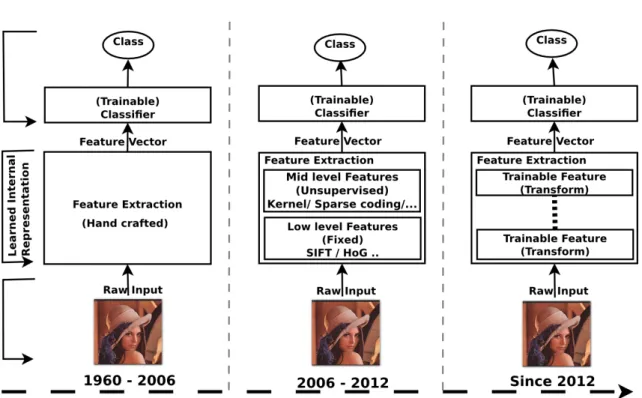
In this section we briefly discuss the major trends of feature extraction methods in the Machine Learning field starting from the early 1960’s to the present day. From a literature survey and keyword usage search, we identified major trend changes in the perspective of the machine learn-ing community and categorized these trends into three evolutionary stages of feature extraction methods. A timeline depiction of these trends along with their evolution is shown in Figure 2.1.

From the early 1960’s till 2006, the community answered queries on how to build methods which transform the collected raw data into a form that a computer can handle. These are first generation feature extraction methods appearing at a time when feature extraction was considered as a field only for specialists who generally used carefully handcrafted features for each learning problem.

(36)

Figure 2.1: Evolution of feature extraction methods from 1960’s to 2015.

Around 2006 the community devised low level feature extractors like Scale-Invariant Feature Transform (SIFT) (Lowe, 1999), Histogram of Oriented Gradients (HoG) (Dalal and Triggs, 2005) for object recognition, and Mel-Frequency Cepstral Coefficients (MFCC) (Davis and Mermelstein, 1980) for speech recognition. These methods were used in a wide variety of applications, thus heralding the second generation of feature extraction methods. SIFT is called a local feature de-scriptor and allows a point inside an RGB2_{image to be represented robustly by a low dimensional}

vector. When you take multiple images of the same physical object while rotating the camera, the SIFT descriptors of corresponding points are very similar in their 128-D space. After the community shifted towards more ambitious object recognition problems and away from geometry recovery problems, we had a flurry of research in Bag of Words, Spatial Pyramids, Vector Quanti-zation and machine learning tools used in any and all stages of the computer vision pipeline. HoG came at a time when everybody was applying spatial binning to bags of words, using multiple layers of learning and making their systems overly complicated. HoG was quite simple and well understood since it was a linear Support Vector Machine (Tomasz, 2015).

In 2012, the community at large began asking how machines can self-learn representations from data. For example, represented data must be in the space of the learner such that it can be classified. This led to a third generation of feature extraction methods in the form of Trainable Feature Transform, which substitutes traditional handcrafted feature extraction with automated feature extraction. To illustrate, when Trainable Feature Transform understands a scene of a man standing, it first learns by distinguishing the pixels of the man with the background, then the lines or edges and finally the object of the man (Bengio, 2009). This has become a new model

(37)

2.1 Trends in feature extraction methods in ML 11

for representing data, which is generally based on deep neural network architectures and more popularly known as Deep Learning.

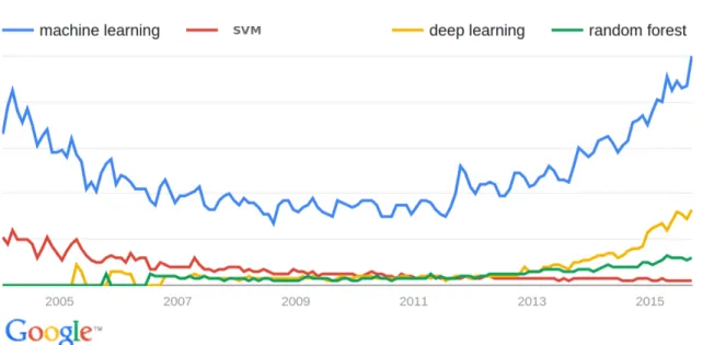
What about other widely used algorithms? Machine learning algorithms such as decision trees, nearest neighbor, logistic regression, Bayesian network, multi-layer neural networks, sup-port vector machines (SVM), and random forest may indeed produce reasonably effective meth-ods for a vast array of applications but are limited by feature extraction methmeth-ods that are mostly handcrafted or have low-level features. To understand the state-of-the-art trends in the machine learning field, we conducted a survey using Google keyword search on worldwide data for the last 10 years with respect to most popular algorithms such as support vector machines, deep learning and random forest. We observed that around the year 2012 the field of Machine Learning gained popularity along with deep learning and random forest algorithms (See Figure 2.2, full report on

Google Trends) (Google, 2015). To understand these trends in detail, we further studied vari-ous applications and competitions held in the field of Machine Learning. We observed that deep learning was not only used in a wide variety of applications, but also revolutionized the Machine Learning field in the past decade.

Convolutional Neural Network (CNN) (LeCun et al., 1998) is a machine learning algorithm belonging to the family of deep neural networks whose architecture of alternating convolutional layers and subsampling layers was inspired by the alternating structure of simple and complex cells in the primary visual cortex (Hubel and Wiesel, 1959). Below is a list of applications in particular to competitions won by CNN among all other algorithms like Decision Trees, Near-est Neighbor, Support Vector Machines, Random ForNear-est and Bayesian Networks. For more on current state-of-the-art results in object classification visit Rodrigo Benenson’s website http: //rodrigob.github.io/ (Benenson, accessed January 12, 2016).

Application: [Year] competition (Group won)

• Handwriting recognition:[Many] MNIST & Arabic (IDSIA)

• Volumetric brain image segmentation: [2009] connectomics (IDSIA, MIT) • OCR in the Wild [2011]: StreetView House Numbers (NYU and others) • Traffic sign recognition: [2011] GTSRB competition (IDSIA, NYU) • Breast cancer cell mitosis detection: [2011] MITOS (IDSIA) • Human Action Recognition: [2011] Hollywood II dataset (Stanford) • Scene Parsing: [2012] Stanford bgd, SiftFlow, Barcelona (NYU) • Speech Recognition: [2012] Acoustic modeling (IBM and Google) • Pedestrian Detection: [2013] INRIA datasets and others (NYU) • Large Scale Visual Recognition: [2013] ImageNet dataset (NYU) • Large Scale Visual Recognition: [2014] ImageNet dataset (GoogLeNet) • Large Scale Visual Recognition: [2015] ImageNet dataset (MSRA, AMAX)

These achievements were made possible due to a breakthrough in training neural nets to self-learn the representation one layer of neurons at a time from a large number of training samples (labeled and unlabeled) without overfitting. This made deep learning appear more efficient when

(38)

Figure 2.2: Worldwide interest over time in the field of Machine Learning with Deep learning, Support Vector Machines and Random Forest. Keyword usage trends from 2004 to present.

compared to other algorithms. This ability along with the availability of low cost parallel com-putational capabilities developed wide acceptance among varied machine learning groups all over the world.

Let’s begin by understanding what is deep learning. To learn the skill of running one has to know the basics of balancing and walking. Similarly, deep learning intends to first learn the basic representation structures and then reuse these structures to develop more specific and abstract feature representations of the data. Deep Learning allows computational models that are composed of multiple processing layers to learn representations of data with multiple levels of abstraction (LeCun et al., 1998).

In the next subsections we discuss some of the popular deep learning methods: Convolutional Neural Networks (LeCun et al., 1998), Stacked Denoising Autoencoders (Vincent et al., 2010) and Deep Belief Nets (Hinton et al., 2006).

2.1.1 Convolutional Neural Networks (CNN)

The research of Neocognitron by Fukushima et.al, introduced CNN as a self-organizing neural network which is unaffected by shift in position for pattern recognition (Fukushima, 1980). This work was later improved by Yann Lecunn et.al, by training a multi-layer neural network with the back-propagation algorithm for gradient based learning (LeCun et al., 1998).

Convolutional Neural Networks take advantage of the fact that the input consists of images by constraining the architecture in a more sensible way. In particular, and unlike a regular Neural Network, the layers of a CNN have neurons arranged in three dimensions: width, height, and depth. (Note that the word depth here refers to the third dimension of an activation volume, not

(39)

2.1 Trends in feature extraction methods in ML 13

to the depth of a full Neural Network, which can refer to the total number of layers in a network.) The CNN architecture transforms the full image into a single vector of class scores, arranged along the depth dimension. This process is illustrated in Fig 2.3.

Figure 2.3: Left: A regular 3-layer Neural Network. Right: A CNN arranges its neurons in three dimensions (width, height, depth), as visualized in one of the layers. Every layer of a CNN transforms the 3D input volume to a 3D output volume of neuron activations. In this example, the red input layer holds the image, so its width and height would be the dimensions of the image, and the depth would be three (Red, Green, Blue channels) (Li and Karpathy, 2015).

CNNs exploit spatially-local correlation by enforcing a local connectivity pattern between neurons of adjacent layers. The architecture thus ensures that the learned filters produce the strongest response to a spatially local input pattern. Also, sharing weights increases the invari-ance of learned filters by replicating each filter across the entire visual field. These replicated filters share the same parametrization (weight vector and bias) and form a feature map. Replicat-ing units in this way allows for features to be detected regardless of their position in the visual field. Additionally, weight sharing increases learning efficiency by greatly reducing the number of free parameters being learned. The constraints on the model enable CNN to achieve better generalization on vision problems.

2.1.2 Stacked Denoising Autoencoders (SDA)

An autoencoder is a simple neural network with one hidden layer designed to reconstruct its own input. For that reason, it hs an equal number of input and output neurons. The learning ac-curacy is obtained by minimizing the average reconstruction error between the original and the reconstructed instances. The encoding and decoding feature sets (input-hidden and hidden-output weights, respectively) may optionally be constrained as transposes of each other. In this case the autoencoder is said to have tied weights. A denoising Autoencoder (dA) (Vincent et al., 2008) is a variant of the autoencoder where now a corrupted version of the input is used to reconstruct the original instances. Moreover, the dA makes an excellent building block for deep networks (Bengio, 2012, Section 5.4). Stacking multiple dA’s one on top of each other gives the model the advantage of hierarchical features with low-layer features represented at lower layers and higher-layer features represented at upper higher-layers (Bengio, 2012, Section 3).

(40)

2.1.3 Deep Belief Nets (DBN)

Deep Belief Nets are a specific type of energy-based model that attempts to learn low-energy state for a desired variable (Salakhutdinov and Hinton, 2009). The DBNs are a fully general Boltzmann machines (Hinton et al., 1984), in which the connections between the hidden units are restricted in such a way that the hidden units form multiple layers. Restricting the fully connected network in Boltzmann machines improves the speed and accuracy, latter coined as restricted boltzmann machines (RBM) (Salakhutdinov et al., 2007). Using a greedy layer-wise pre-training (Hinton et al., 2006) for training stacked RBM paved the way for Deep architectures leading to Deep Belief Nets (Hinton et al., 2006) and Deep Boltzmann Machines (Salakhutdinov and Hinton, 2009). DBNs perform better than the Stacked Autoencoders in cases where they have access to prior probability distribution are available (Holst et al., 2015).

2.2 Model for Transfer Learning in ML

The initial works on transfer learning began with the 1995 NIPS workshop. The Defense Ad-vanced Research Projects Agency (DARPA) funded in 2005 a Transfer Learning (TL) program to increase the interest in TL challenges and potential contributions (Gasser et al., 2005). The Multitask learning by (Caruana, 1997) explores the simultaneously learning of multiple tasks by sharing the weights of the network. The core idea of sharing weights increases learning of model that solves many tasks with good generalization. The Multitask Learning approach is different from multiclass learning, the model learns c different output variables {Y1,Y2, ...,Yc}

correspond-ing to n different tasks. The Multitask Learncorrespond-ing learns multiple source tasks simultaneously by sharing the knowledge (features) between the tasks or conditional models.

In Lifelong Learning, multiple related source tasks are learned one after another by the model in an incremental approach; to solve for nth (target) task the model needs to learn serially all source model tasks up to the (n − 1) task. The previous learning helps to solve the new target task. However, if the source task(s) are not related to the target task causes degraded performance. It is also limited by the order in which the source tasks are presented. Learning to Learn (Thrun and Pratt, 2012) is a variation of Lifelong Learning (Thrun, 1998). The main intuition of this model is based on learning many tasks serially, one after another, under the assumption that learning the n-th task may be easier than the (n − 1)-th task.

A large number of works have been produced with the name Domain Adaptation like (Blitzer et al., 2006), (Jiang, 2008), (Patricia and Caputo, 2014), (Ben-David et al., 2010) and (Bruzzone and Marconcini, 2010). Domain adaptation is a transfer learning framework which adapts the learner such that tasks between correlated domains3 perform better than uncorrelated domains.

3_{The correlation between probability distributions (which allows estimating quantitatively how similar they are)}

can be empirically evaluated according to some similarity metrics. Hence, two domains are considered correlated if the distance between the corresponding underlying distributions is relatively small according to proper metrics, see (Bruzzone and Marconcini, 2010).

(41)

2.2 Model for Transfer Learning in ML 15

Domain adaptation expects that the closer the distributions of the problem are, the better the fea-tures trained on the source problem will perform on the target problem, thus limiting transfer learning problems to those for which the distributions are closely related.

Some traditional machine learning models can be used under different conditions for TL prob-lems, like Semi-Supervised Learning, Ensemble methods, Bayesian priors, and meta-learning. The Semi-Supervised Learning explores how to learn from both labeled and unlabeled data, thus transferring the knowledge from source labeled data to the target unlabeled data (Zhu, 2006). The traditional Ensemble method combines a set of models to construct a complex classifier for a clas-sification problem. Ensemble methods can be directly used in TL models by building the set of models from different distributions or tasks or problems. The various ensemble approaches and its solutions are discussed in (Jiang, 2008). Traditionally, in Bayesian priors models, we use a maximum a posterior (MAP) estimation approach for supervised learning to get Bayesian pri-ors distributions. If the Bayesian pripri-ors are computed from the source domain labeled instances then this approach can be used easily for many TL problems. Even classical machine learning techniques such as rule induction may be easily leveraged to assist with TL applications. In meta-learning the reuse of meta-features (knowledge) or properties of the model is utilized to solve a new task (Vilalta and Drissi, 2002). Listed below are the most common methods for TL problems with unlabeled data (Zhu, 2006):

1. Use a trade-off parameter between the labeled and the unlabeled data. The trade-off param-eter is calculated with Kullback-Leibler divergence4_{between the domains.}

2. Use of a instance weighting method to factorize in both source labeled and target unlabeled instances during training.

3. Use of label propagation for unlabeled target data on a nearest neighbor graph.

Here we focus on the knowledge transfer based on the several survey works in the past decade discussing on overview and applications of transfer learning. The survey by Pan et.al, discusses several transfer learning frameworks including classification, regression, and clustering approaches in inductive, transductive, and unsupervised transfer settings (Pan and Yang, 2010). The difference between inductive and transductive learning is that the inductive learners can nat-urally handle unseen data, whereas the transductive learning will be used to contrast inductive learning. A learner is said to be transductive if it works only on the labeled and unlabeled training data, and cannot handle unseen data. Survey works of Van otterlo et.al, on TL for reinforcement learning are specific for relational domains (Van Otterlo, 2005) and another survey on reinforce-ment learning specify about the relation between between domains with only limited environ-mental feedback rather than correctly labeled examples (Taylor and Stone, 2009). Many specific transfer learning applications have been studied in detail: in activity recognition by (Cook et al.,

4_{Kullback-Leibler divergence measures the similarity of some distribution P to another distribution Q. It is not}

(42)

2013), in bioinformatics by (Xu and Yang, 2011) and in Cross-domain collaborative filtering by (Li, 2011).

Studying the various surveys on TL we summaries the main goal of TL is to transfer the knowledge (learning) obtained from a source domain to one or more target domains in order to efficiently develop an effective hypothesis for a new task, domain or distribution (Ben-David et al., 2010). Brute-forcing knowledge from the source domain into the target domain, irrespective of their divergence, may cause a certain performance degradation or, in even worse cases, break the original data consistency in the target domain called as negative transference (Shao et al., 2015) or the performance the may exceed than the no transfer network (baseline approach) called as positive transference. This ambiguity in performances raises general issues regarding the transfer process: when to transfer?, what to transfer?, and how to transfer?

The answer to when to transfer includes the issues whether transfer learning is necessary for specific learning tasks and whether the source domain data is related to the target domain data. In scenarios where the training instances are sufficient, impressive performance can be achieved without any type of knowledge transference. However, we need to build models which adapt the gained knowledge to these scenarios in order to improve the overall performance of the new tasks. The answer to what to transfer can be summed up in three approaches: the inductive transfer learning, using all the source domain instances and their corresponding labels for knowledge trans-fer; the instance transfer learning, relying mostly in the use of source domain labeled instances and also sometimes in target domain unlabeled instances; and the parameter transfer learning, using model parameters or hyper-parameters of the source domain for faster and accurate modelling of the target domain.

The answer to how to transfer includes all the specific transfer learning techniques. Knowl-edge transfer is based on the non-negative matrix trifactorization framework. The transfer learning phase is performed via dimensionality reduction (Shao et al., 2015). The most widely used meth-ods transfer not only features but also parameters and hyper-parameters to the target domain.

In the literature, the term TL is used by different groups under different names and/or defini-tions. To have all these definitions under a single framework is challenging. In here, we use the most common underlying phenomena of TL that is very simple and generic among all the different definitions. We reuse the knowledge learned from a problem, or a set of problems, in a way that the knowledge gained helps to solve the new problem(s) more effectively. Inside this broad defi-nition of TL, in the next section we discuss various methodologies for solving the above general issues that have been previously explored in the context of deep neural networks.

2.3 Challenges in Deep architectures using Transfer Learning

In recent years, there has been a growing interest in deep architectures for TL applications. One such interesting study inquired on how transferable are the lower layers’ (generic) versus higher

(43)

2.4 Conclusions 17

layers’ (specific) features in the hierarchical deep network (Yosinski et al., 2014). Another impor-tant work studied unsupervised TL using stacked autoencoders on a deep architecture model (Glo-rot et al., 2011). Concept drift is a study that incorporate the change in environment for big data (Gama et al., 2014). The feature transference approach for transferring top level CNN fea-tures for various object recognition problems have performed better in most of the cases (Razavian et al., 2014).

Even with good performance with most of the problems we foresee many shortcomings of these types of approaches: 1) the tasks have to be related, 2) the feature space and the learning space of the problem must be the same. Despite the vast body of literature on the subject (see (Glo-rot et al., 2011), (Bengio et al., 2013), (Bengio, 2012), (Ciresan et al., 2012)), there are still many contentious issues regarding TL problems from different distributions. TL methods, especially domain adaptation (Glorot et al., 2011) and multi-task learning (Bengio et al., 2013), are based on the assumption that both source and target problems are drawn from a related distribution. Even self-taught learning, which uses unlabeled data to train, needs both the source and the target datasets to be from the same modality (the input must be either image, audio or text only) (Raina et al., 2007).

Here we summarize the main challenges that are faced by the deep learning community using transfer learning approaches:

1. How transferable are the supervised and/or unsupervised features for correlated or uncorre-lated domains?

2. How do we avoid or reduce the feature transferability that may lead to negative transference? 3. Is it possible to have transference across different network architectures? e.g. the number

of layers and/or number of neurons.

4. Is it possible to have transference between different modalities? e.g. image to text or text to sound, etc.

5. Is it still possible to have effective TL in the case of large number of a target data training samples?

6. How do we select the target model if there are multiple models from different source domain problems?

2.4 Conclusions

It can be seen throughout the history of machine learning that some algorithms do better than others, but what makes the difference? Easily, the most important factor is the ability of machines to interpret data like humans. Then, how to enable machines to efficiently represent data without human interaction? Also, how to reuse the knowledge gained by learning problems to solve a new problem? The key to answer such questions may be in deep learning using TL approaches. Our

(44)

analysis of feature extraction methods and knowledge transference in terms of their capabilities and goals leads to this conclusion.

As guidance for future directions of this research work, we intend to utilize generic feature representations obtained by deep learning methods for multiple problems, tasks, or domains using the TL approaches. These computationally expensive hierarchical models trained on very large datasets will be harnessed. First we using parallel processing hardware that has scalable compu-tational power like GPUs that provide higher performance of watt per bit. Second we improve the algorithm to use faster optimization techniques and TL approaches. In the subsequently chap-ters we discuss our proposed approaches and original contributions that would mitigate previously discussed challenges.

(45)

Part II

Deep Transfer Learning Mechanisms

(46)

(47)

Deep Transfer Learning Framework 21

Chapter 3

Deep Transfer Learning Framework

In this chapter our objective is to present an introduction of the basic Deep Transfer Learning con-cepts and techniques for classification of image based problems. We begin by introducing some of the necessary terminology and by describing fundamental concepts and operations associated with the process of transferring source problem knowledge (features) to target form suitable for training machines. In this chapter we discuss the deep transfer learning methodology that over-comes the multi-layer perceptrons limitation of overfitting and utilize a transfer learning technique for training on large unlabeled data samples. Some parts of this chapter are used in (Kandaswamy et al., 2014b) and (Kandaswamy et al., 2014a).

3.1 Fundamental concepts of deep learning

Deep Neural Networks (DNN) are very similar to ordinary Neural Networks (NN). NNs receive an input (a single vector) and transform it through a series of hidden layers. Each hidden layer is made up of a set of neurons, where each neuron is typically fully connected to all neurons in the previous layer, and where neurons in a single layer function completely independently and do not share any connections. The last fully-connected layer is called the “output layer” and in classification settings it represents the class scores. NNs do not scale well to full images: the full connectivity is wasteful and the huge number of parameters would quickly lead to overfitting. Similarly, DNN’s are made up of neurons that have learnable weights and biases. Each neuron receives some inputs, performs a dot product with a weight vector and optionally applies a non-linear function. The whole network still expresses a single differentiable score function: from the raw image pixels on one end to class scores at the other. And they still have a loss function (e.g. Softmax) on the last (fully-connected) layer and all the tips/tricks we developed for learning regular Neural Networks still apply:

1. Learning method: Let us define a dataset by a set of tuples D = {(xxxi, yi)}N_i=1, xxxi∈ XN, yi∈

YN. The set XN= {xxx1, ..., xxxN} contains N instances of a d-dimensional random vector X ⊆

Rd. Similarly, the set YN = {y1, . . . , yN} contains N instances of a one-dimensional random