A Work Project, presented as part of the requirements for the Award of a Master Degree in Economics from the NOVA-School of Business and Economics
The Impact of the Single Currency on Economic Growth
João Gonçalo Landeira da Silva ,3112
A project carried out on the Master in Economics Program, under the supervision of: Miguel Lebre de Freitas
2
The Impact of the Single Currency on Economic Growth
João Gonçalo Landeira da Silva
Abstract
Did the creation of the euro affect economic growth? To address this question, we estimate a simple growth model and we found an insignificant impact of the euro on GDP per head however when we look for differentiated impacts the GDP growth of the six members that founded the European Union was negatively affected by the creation of the euro across all period. Lastly, the GIIPS were the only group statistically affect by the crisis when we look to the impact of it in different groups.
Keywords: Euro, Economic Growth, Fixed Effects
Acknowledgements:
I would like to thank my advisor, Professor Miguel Libra de Freitas, for the guidance and patience that allowed me to finish this work. Specially, want to thank my family for all the love and support . I also want to thank my friends Pedro Silva, João Oliveira, Henrique Oliveira and Ricardo Santos for all the shared support and thoughtful ideas .
3 1.Introduction
The advent of the euro was the next step of European Union integration, a joint currency that allowed companies to easily trade between members states, less uncertainty not only for companies, but also for regular citizens that would have more freedom of choice and from that we could hope for a positive impact in economic growth. The euro in fact can positively affect income and efficiency, since it allows more macroeconomic stability through lower exchange rate volatility, higher transparency on financial markets and discipline enhancing fiscal rules. It also contributes to higher efficiency through trade since integration promotes competition that has a positive effect on physical and human capital and therefore on growth (Baldwin,1992).
On the other hand, the euro does not allow each country to devalue their currency and this can be problematic for countries facing asymmetric shocks. Problems like this lead some opinion makers to defend more integration to close the gaps between countries while others contest that the euro is impaired and their countries most leave the euro.
Considering all these divergent effects that the euro might have, after 18 years of integration, to our knowledge, no work has tried to access whether EU Membership made a difference for economic growth. In this paper, we use a cross section estimation like Barro (1991) but using Panel Data to investigate to what extent the creation of euro affected economic growth and if in fact the periphery’s economic growth has been that much damaged by the single currency.
We use a Fixed Effect Model with data from all OECD countries to estimate a basic model with capability to predict real GDP growth, methodology used by Easterly (2005) and recently by Checherita-Westphal and Rother (2010), among others. Then augmented it by introducing a dummy for Euro Area expecting to capture the effect of the single currency on Economic Growth. A similar method was used by de Sousa and Lochard (2011) to investigate
4 whether the single currency positively impacts Foreign Direct Investment. We also want to access the impact of the euro in different groups of countries, however we are not interested in capture the idiosyncrasy of each country, each is a question in the scope of member state policy. The work is organized as follow; section 2 reviews the relevant literature; Section 3 describes the data and the methodology used; Second 4 presents the empirical result; Section 5 concludes.
2.Literature Review
To our knowledge, nobody tried to access if the EA membership has an impact on growth after controlling for other effects. The euro was the great political happening of this century and countries that entered the euro zone expected returns from implementation of the euro, and one of those is certainly more economic growth.
The single currency has as benefits exchange rate certainty, more integrated financial markets and price stability (Mundell,1961). Adding to this it is view that a country decentralized monetary authority will be more able to commit to monetary rules (Silva and Tenreyro, 2010). For this reason, the euro can positively influence income through more macroeconomic stability. When trade partners are in the same currency area conversion costs are eliminated, therefore they will have lower transaction costs and a deeper integration in goods and capital markets is expected ( Glick and Rose (2016) finds a positive impact between the European monetary Union and trade). And larger markets will increase competition (also enhanced by higher price transparency) between companies and that will optimally result in increase of efficiency in the use of physical and human capital (Baldwin, 1992). These conditions can, for example, increase investment flows towards these countries, however FDI does not have a positive impact on growth that is independent of other growth determinants (Carkovic and Levine, 2002).
5 The euro is not an optimal currency area (Grauwe 2006) it incorporates some problems that can be harmful for growth and that opinion makers use eagerly to criticize the euro. Namely, asymmetric shocks, in face of price rigidities may lead to macro instability that is harmful to growth. For some countries, cost may exceed benefits. Hence, our research.
Growth theoretical literature can be traced back to Ramsey (1928), neoclassic model is still important to explain the convergences forces where poor countries tend to catch up to rich ones (Solow ,1956). However, there is a consensus in the literature that: (i) growth can be affected by accumulation of capital through more investment in physical, human capital and R&D; (ii) growth is associated with technological progress; (iii) differences in growth can be explained by macroeconomic environment, i.e., the quality of policies and economic institutions (Barro, 2013). Therefore, the euro can positively affect growth by improving the quality of the economic environment enhancing incentives to produce and invest.
Many studies tried to capture the effects of policies and institutions on economic growth. After the surge of endogenous growth models there has an outbreak of empirical estimation of growth models using cross-country data. Barro (1991) related initial level of per capita output and other variables with economic growth using a simple cross-country model. Barro (1991) found evidence of conditional convergence estimating the model with variables of initial income level and controlling for education, school enrollment at secondary and primary levels (proxy for human capital).
More recent papers of economic growth use a panel data methodology to exploit time series and cross-sectional variation, approach that is closer to what I want to study since to analyze the impact of the euro on growth we need time variance but at the same time need to control for the behavior of non-euro economies.
Checherita-Westphal and Rother (2010) used a fixed effect model for a panel data of 12-euro area economies from 1970 to 2011 and found a non-linear impact of government debt
6 on growth of per capita GDP. They estimate for growth rates of one year and cumulative overlapping and non-overlapping growth rates of five years to capture long term impacts. So, at the end they found evidence that, in the euro area, high government debt negatively affects yearly growth but also longer-term growth. Easterly (2005) tried to measure the impact of policies on five-year average real per capita growth between 1960 and 2000, using various methods he found that only extreme policies (for example, high inflation) would have an impact in growth, despite that in the fixed-effect approach we found that the variables inflation, black market premium as well as currency overvaluing are the only variables to have relevant within variation.
Grauwe and Ji (2016) relates economic growth with rigidities in labor market using a sample of 32 OECD countries, and states, controlling for variables like government consumption, investment ratio to GDP and the proportion of population with tertiary education, that employment protection does not have a clear importance on growth, and that it cannot be the reason to explain the poor performance (after 2010) of the euro zone in growth terms when compared with the rest of the European Union and USA but instead, he argues, that it must be related with demand sided problems and the fact that the adjustment process being all supported by the debtor countries drove the euro economy to stagnate.
In the literature there have been already attempts to account for the EA membership using fixed effects, Sousa and Lochard (2011) used a gravity model to estimate the impact of the creation of the eurozone in bilateral foreign direct investment (FDI). Using a panel of 21 countries between 1992-2005 they estimated the effect of a Dummy for the Euro in a Fixed effect model controlling for other variables that are likely to effect FDI. Doing several robustness tests their dummy kept the statistical relevant positive effect what led them to conclude that the Euro “has increased intra-EMU FDI stocks on average by around 30 percent”. Glick (2016) also used a gravity model but to measure the impact of the euro on trade. Using a
7 panel data of more than 200 countries and controlling for time-varying country and dyadic fixed effects he found that European Monetary Union expanded European trade around 50% and that the impact of EMU is higher for the older countries of the euro than for the newer. Our paper differs from these because we address the impact in growth.
3 Methodology 3.1. Model
The basic estimation is panel fixed-effects corrected for heteroskedasticity and autocorrelation. The equation for the baseline model is below.
𝑔𝑖𝑡5 = 𝛼 + 𝑋𝑖𝑡−5′ 𝛽 + 𝜇𝑖+ 𝜗𝑡+ 𝜀𝑖𝑡 (1)
Where 𝑋𝑖𝑡−5′ stands for the vector of control variables and 𝛽 the vector of Coefficients. The model controls for the conditional convergence test present in Mankiw, Romer, and Weil (1992), i.e., controls for population growth and investment in human and physical capital while measuring the impact of initial per capita income in economic growth. It is augmented to include other variables that appeared with endogenous growth literature like measures of economic policy quality and economy openness in line with Sachs and Warner (1995). Then we also add country dummies to control for the impact of the euro or the crisis in economic growth.
My dependent variable will be 5-year cumulative overlapping growth rate. Five-year growth rate allows me to avoid cyclical movement, and mitigates reverse causality, normally present in these models, since 5-year growth cannot determinate variables in the beginning of the cycle. So, we use a model with 5 years growth rate based on independent variables in the beginning of the cycle.
8 So, the following model would be able to predict economic growth:
𝑔𝑖𝑡5 = 𝛼 + 𝛽1ln(𝐺𝐷𝑃 𝑝𝑒𝑟 ℎ𝑒𝑎𝑑)𝑖𝑡−5+ 𝛽2 𝑝𝑜𝑝𝑔𝑟𝑖𝑡−5+ 𝛽3 𝐼𝑛𝑣𝑒𝑠𝑡𝑚𝑒𝑛𝑡𝑖𝑡−5+ 𝛽4 𝑒𝑑𝑢𝑐𝑖𝑡−5 + 𝛽5𝑔𝑜𝑣. 𝑐. 𝑔𝑖𝑡−5+ 𝛽6 𝑖𝑛𝑓𝑙𝑎𝑡𝑖𝑜𝑛𝑖𝑡−5+ 𝛽7 𝑂𝑝𝑒𝑛𝑖𝑡−5
+ 𝛽8 𝑔. 𝑡𝑒𝑟𝑚𝑠𝑜𝑓𝑡𝑟𝑎𝑑𝑒𝑖𝑡+ 𝜇𝑖 + 𝜗𝑡+ 𝜀𝑖𝑡 (1)
Where 𝑔𝑖𝑡5 is the real GDP growth rate in 5 year time, ln(𝐺𝐷𝑃 𝑝𝑒𝑟 ℎ𝑒𝑎𝑑)𝑖𝑡−5 stands
for the natural logarithm of the GDP per head of population aged 15-64 years, 𝑝𝑜𝑝𝑔𝑟𝑖𝑡−5 is
population growth (between 15-64 years), 𝐼𝑛𝑣𝑒𝑠𝑡𝑚𝑒𝑛𝑡𝑖𝑡−5 is gross fixed capital formation (% GDP), 𝑒𝑑𝑢𝑐𝑖𝑡−5 is my proxy for human capital.
We included also some variables to proxy policy choices1: (i) Government non-productive consumption(𝑔𝑜𝑣. 𝑐. 𝑔𝑖𝑡−5), that is interpreted as a bad policy decision, so it is expected to have a negative impact on growth ; (ii) inflation (𝑖𝑛𝑓𝑙𝑎𝑡𝑖𝑜𝑛𝑖𝑡−5) computed as ln(1+ Inflation rate): normally this value as to be lagged to avoid reverse causation, so that lower growth leads to higher inflation, but since we are looking at 5-year growth rate and present level we think there is no need. We also introduced, to expand the model beyond close economy, an indicator of openness (𝑂𝑝𝑒𝑛𝑖𝑡−5) and terms of trade growth rate (𝑔. 𝑡𝑒𝑟𝑚𝑠𝑜𝑓𝑡𝑟𝑎𝑑𝑒𝑖𝑡)(both
expected to have a positive impact in growth). Terms of Trade growth rate in the regression won’t be the initial value but instead a 5-year growth rate computed in the same away as the GDP growth rate. The country dummies (𝜇𝑖) in the equation capture specific economic and
social characteristics, that remain relatively constant over time. Furthermore, included year dummies (𝜗𝑡) to control for common shocks across countries, like the 2008’s crisis.
1 We also used an Indicator of Quality of economic institutions from KUNČIČ (2014), it was statistically
significant however it made the other variables economic insignificant and did not changed the final conclusion, so we decided to not include it on the model
9 The baseline model after will be augment by introducing a Dummy for the Euro Area, i.e., a dummy that takes the value of 1 if at t the country uses euro as his currency and 0 otherwise.
𝑔𝑖𝑡5 = 𝛼 + 𝑋𝑖𝑡−5′ 𝛽 + 𝐸𝐴𝑖,𝑡−5 + 𝐸𝑈𝑖,𝑡−5 + 𝜇𝑖 + 𝜗𝑡+ 𝜀𝑖𝑡 (3)
EA is the dummy for the Euro Area at t-52. EU that is equal to 1 if the country is member of the European Union at t and 0 otherwise. Further we also control for other impacts like the crisis using dummies.
The choice of within estimation allows me to answer the question: “Does adopting the euro affect Economic Growth?”, the fact that the within estimation exploits time-series properties of the data takes us to estimate the impact of the euro by comparing the evolution of the GDP per head growth before and after a country enter the single currency.
3.2. Data and Variables
We want to investigate the impact on real GDP per head of population aged 15-64 years growth of the euro’s introduction in the euro area economies. Our dataset has a total of 35 OECD countries. Unlike World Samples our sample does not have large heterogeneity so there is no need to control for variables like region, conflicts or ethnicity. The dataset covers data from 1985 until 2015, we computed GDP per head of population aged 15-64 years expressed in Purchasing Power Parities with data from the OECD.Stat Database and the World Bank Database. The use of real GDP per working age person allows us to mitigate growth differences that are related with demographics and focus on the ability that the economies have to make the
2 EA considers the following countries: Austria, Belgium, Finland, France, Germany, Greece, Ireland, Italy,
10 most of available human resources, since it does not make distinctions between people employed, unemployed or out of the labor force (de Freitas, Pereira, and Torres , 2003).
To proxy human capital I used an education variable, even though there is no consensus on the best proxy for human capital education is broadly used as a proxy, however a variable is difficult to find since the most used and commonly accepted variables are only availed from 5 to 5 years, so we opted for a variable from the United Nations Educational, Scientific, and Cultural Organization: Gross enrollment ratio; that is the ratio of total enrollment, regardless of age, to the population of the age group that officially corresponds to the level of education shown, in this case tertiary education. High education might be better to measure the differences between OECD countries (Grauwe and Ji (2016) finds Proportion of tertiary education to be positively correlated with the growth rate of per capita GDP).
Trade Openness is measured as the sum of Imports and Exports of goods and services divided by GDP3. While General government final consumption expenditure (data extracted from World Bank and OECD national accounts data) includes all government current expenditures for purchases of goods and services, as a ratio of GDP. From the International Monetary Fund, we obtained data on Inflation measured by the consumer price index annual change and Terms of trade is the ratio between index export prices and index import prices. Also added a measure of Gross measured as percentage of GDP using the available data from World Bank.
3 Stressing that the ratio is normally higher for smaller countries, Barro (2013) defends that this basic measure
would not reflect policy influences, nevertheless we decided to keep it since it is widely use in growth
regression, and other measures proposed by Sachs and Warner (1995) are not adequate to panel regression since thy do not have enough within variation.
11
Table 0- Descriptive Statistics
VARIABLES N mean sd min max
Log (Initial GDP) 1,039 10.69 2.122 5.236 16.26 Government Consumption 1,034 0.187 0.0426 0.0752 0.363 Education 983 0.506 0.226 0.0244 1.139 Openness 1,034 0.805 0.489 0.160 4.195 Investment 1,034 23.04 % 4.055% 11.55% 39.40% Inflation 1,033 0.0607 0.130 -0.0458 1.880 Population Growth 1,085 0.00635 0.00985 -0.0586 0.0670
Terms of Trade Growth rate 863 0.0141 0.0928 -0.298 0.806
𝑔5,𝑡 999 0.117 0.123 -0.249 0.633
4. Results
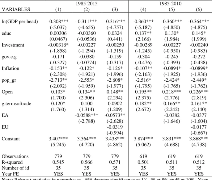
In Column (1) from Table 1 are reported the results from equation 2, the model explains a reasonable part of the within variation (within R-squared is 0.545) and is clustered at the country level. Across the different regressions the natural logarithm of GDP shows statistical significant coefficients that have the negative expected sign, so the model has evidence of conditional convergence, controlling for other variables when GDP per head increases the country expects lower GDP growth, ceteris paribus. Education has the expected positive sign, nevertheless is not significant. The first thing that strikes is a negative impact of gross fixed capital formation (even if only marginally significant) 4.Government consumption shows the
expected negative sign, for the reasons explained above. Both inflation and population growth have the expected negative sign, so for the given values of initial level of GDP and controlling for other variables it is expected that higher inflation and higher population growth imply lower economic grow, at a 5% significance level. As referred above the importance of openness to
4 We regressed all the equations in Table 1 without the Investment variable, but the outcomes did not change so we decided to keep it on the model. Checherita-Westphal and Rother (2012) also find this negative relation in their five-year cumulative fixed effect between growth and private gross fixed capital formation while public wasn´t statistically relevant.
12 growth is capture on the Trade Openness and Terms of Trade growth rate coefficients, since both have positive signs, being both statistically relevant, at least at 10%.
Controlling for all variables described above the results in column (2) suggest that monetary integration matters. The dummy that considers the entering time of the countries in European Monetary Union (EA) has statistically negative impact in GDP per head growth at 1% significance level when we consider a period between 1985-2015. Ceteris paribus, the adoption of the euro will reduce 5-year real growth rate, on average, by 5,88 percentage points. In column (3), the EA dummy is robust to the introduction of EU membership. EU controls for the European Union in the same away that EA controls for the euro, nevertheless it is not statistical significant.
Since we consider a period until 2015, a major economic crisis is present in our sample: 2008’s crisis somewhat affected all the economies in our sample therefore it must be controlled by the time dummies, on the other hand the effects of this crisis were more persistent on the Euro Area countries ( what led to the further called Sovereign Debt Crisis) and that it is not fully captured by the model, time dummies won´t affectively capture this effect, meaning that the significance of our findings above might be undermined, so we estimated a new model that only captures growth rate until 2010.5
5 Since the Growth rate for t=2011 already accounts for the lower GDP growth induced by the Sovereign Debt
13 In the new regression, column (4), all the control variables keep the expected sign, then controlling for the Euro Area the first thing that strikes is that the dummy is no longer significant, as we can see in column (5) of Table 1. Not a surprise since the 2008’s crisis had a more persistent impact on the Euro Area being this evidence of the problems that these countries had to react to it. Also controlled for the European Union in column (6) however the conclusion is the same.
The first regressions seem to show that the euro had a negative impact on growth however that impact seems to be related with the poorer performance of these economies after 2010 and not before. Instead of having two periods, we created a dummy for the crisis so that
Table 1 – Baseline Model and the Euro Effect
1985-2015 1985-2010 VARIABLES (1) (2) (3) (4) (5) (6) ln(GDP per head) -0.308*** -0.311*** -0.316*** -0.360*** -0.360*** -0.364*** (-5.037) (-4.655) (-4.757) (-5.187) (-4.850) (-4.875) educ 0.00306 -0.00360 0.0324 0.137** 0.130* 0.145* (0.0467) (-0.0536) (0.441) (2.166) (1.984) (1.999) Investment -0.00316* -0.00227 -0.00250 -0.00289 -0.00227 -0.00240 (-1.858) (-1.294) (-1.319) (-1.245) (-0.950) (-0.983) gov.c.g -0.171 -0.0380 -0.159 -0.304 -0.245 -0.272 (-0.327) (-0.0774) (-0.317) (-0.476) (-0.393) (-0.438) Inflation -0.153** -0.122* -0.126* -0.107** -0.0894* -0.0899* (-2.308) (-1.921) (-1.996) (-2.163) (-1.925) (-1.936) pop_gr -2.713** -2.553* -2.608* -2.516* -2.424* -2.449* (-2.092) (-1.959) (-1.977) (-1.795) (-1.765) (-1.762) Open 0.103* 0.134** 0.148** 0.195** 0.218*** 0.226*** (1.700) (2.306) (2.294) (2.375) (2.776) (2.819) g.termsoftrade 0.120* 0.100 0.0902 0.182** 0.166** 0.161** (1.760) (1.314) (1.209) (2.672) (2.242) (2.140) EA -0.0588*** -0.0573** -0.0382 -0.0377 (-2.788) (-2.628) (-1.646) (-1.604) EU -0.0319 -0.0177 (-0.994) (-0.667) Constant 3.407*** 3.364*** 3.438*** 3.874*** 3.831*** 3.868*** (5.245) (4.720) (4.862) (5.062) (4.688) (4.738) Observations 779 779 779 619 619 619 R-squared 0.545 0.566 0.571 0.501 0.511 0.512 Number of id 35 35 35 35 35 35
Year FE YES YES YES YES YES YES
Note: Robust t-statistics in parentheses. *** denotes significance at 1%, ** at 5% and* at 10%. Year Dummies are not reported. Estimations are based on equation (2) augmented to an Euro Area and European Union Dummy
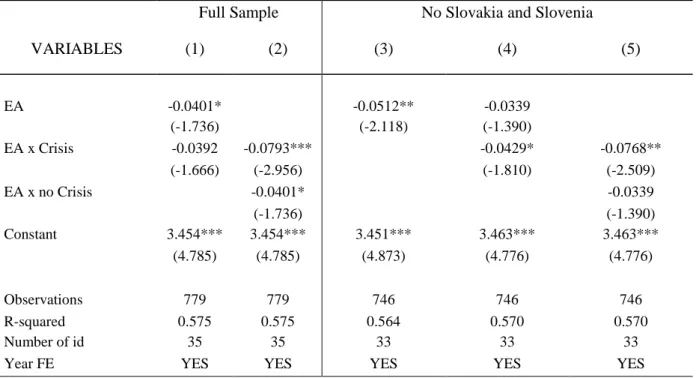
14 it takes the value of 1 if the country is part of the Euro Area after 2010 (EA x Crisis) and a dummy for the Euro Area that does not consider the period after 2010 (EA x no Crisis)6. So, when we have the Full Sample the effect of the crisis is larger than the effect of the period before the crisis. But in this case the crisis dummy also accounts for the euro’s impact on Slovakia and Slovenia, since they have entered in 2007 and 2009, respectively, and due to our methodology, the effect of the euro in these countries is only captured after 2010. And since we cannot accurately separate the effect of the crisis from the two late entries in our sample we drop both from the sample
We can now see that in fact Slovakia and Slovenia were negatively affect by the euro, the coefficient with both countries is -0,058 while without them it is smaller (-0.051)7, and that the period before the crisis is no longer significant, while, holding everything else constant, in crisis years on average GDP per head of the Euro Area countries decreases by 7,68%, in 5 years-time, when compared to non-crisis years. So, when we exclude the Slovakia and Slovenia effect the euro economies experienced lower growth when joining the euro, however this effect is only relevant because of the period that incorporates the Sovereign Debt Crisis, so after 2010.
6 Regressions in table 2
7 We have disproportionate periods of time with euro and without the euro, so it is more likely to find differences
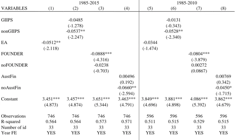
15 When we considered the full period the euro negatively affects real GDP growth, but when we divided in two this lower growth is correlated with the economic crisis and not with the adoption of the euro as a currency by these countries, nevertheless this effect was found statistically relevant for the Euro as a group but indeed it can diverge from to country to country or even form group to group of countries. To investigate these differences, we define different groups and we will try to understand the different impacts of the euro and of the crisis on them. We divided the Euro Area Dummy in 3 different variables: (i) GIIPS that considers Greece, Spain, Italy, Portugal and Ireland;(ii) FOUNDER that considers France, Luxembourg, Italy, Netherlands, Belgium and Germany; (iii) AustFin that considers only Austria and Finland.
Table 2 – Timing of the Effect 1985-2015 with crisis dummy
Full Sample No Slovakia and Slovenia
VARIABLES (1) (2) (3) (4) (5) EA -0.0401* -0.0512** -0.0339 (-1.736) (-2.118) (-1.390) EA x Crisis -0.0392 -0.0793*** -0.0429* -0.0768** (-1.666) (-2.956) (-1.810) (-2.509) EA x no Crisis -0.0401* -0.0339 (-1.736) (-1.390) Constant 3.454*** 3.454*** 3.451*** 3.463*** 3.463*** (4.785) (4.785) (4.873) (4.776) (4.776) Observations 779 779 746 746 746 R-squared 0.575 0.575 0.564 0.570 0.570 Number of id 35 35 33 33 33
Year FE YES YES YES YES YES
Note: Robust t-statistics in parentheses. *** denotes significance at 1%, ** at 5% and* at 10%. Year Dummies and other control variables are not reported. First 2 regressions are for the full sample, in the last 3 Slovakia and Slovenia are dropped. crisis dummy takes value of 1 if the country is part of the Euro Area after 2010
16 In table (4) we regressed equation (3) but instead of EA variable we consider each group above comparing it with the Eurozone economies that don´t belong to that group.8
In column (2) from table 3 we can see that the effect of euro on the GIIPS’ economies is not relevant, so despite common belief that these economies where in a path of lower growth since they joined the euro that it is not what the evidence shows, regardless of the period considered the GIIPS dummy is not relevant, controlling for the set of variables in equation (2).
8 For example, in column (2) in table 3 nonGIIPS is a dummy that includes the countries that are part of the EA
but aren´t in GIIPS group, for example France or Austria. Table 3 – Impact of the Euro in different groups
1985-2015 1985-2010 VARIABLES (1) (2) (3) (4) (5) (6) (7) (8) GIIPS -0.0485 -0.0131 (-1.278) (-0.343) nonGIIPS -0.0537** -0.0528** (-2.247) (-2.340) EA -0.0512** -0.0344 (-2.118) (-1.474) FOUNDER -0.0888*** -0.0804*** (-4.316) (-3.879) noFOUNDER -0.0238 0.00272 (-0.703) (0.0867) AustFin 0.00496 0.00769 (0.192) (0.342) noAustFin -0.0660** -0.0450* (-2.594) (-1.715) Constant 3.451*** 3.457*** 3.651*** 3.463*** 3.849*** 3.881*** 4.086*** 3.862*** (4.873) (4.874) (5.344) (4.791) (4.696) (4.898) (5.392) (4.679) Observations 746 746 746 746 596 596 596 596 R-squared 0.564 0.564 0.573 0.571 0.511 0.515 0.529 0.515 Number of id 33 33 33 33 33 33 33 33
Year FE YES YES YES YES YES YES YES YES
Note: Robust t-statistics in parentheses. *** denotes significance at 1%, ** at 5% and* at 10%. Year Dummies and other control variables are not reported. Groups are GIIPS: Greece, Ireland, Italy, Portugal and Spain; Founder: Belgium, France, Germany, Italy, Luxembourg and Netherlands; AustFin: Austria and Finland; and no Groups are the countries not in that group but that are in the eurozone.
17 On the other hand, non GIIPS and non AustFin dummies are relevant , while the dummy that considers the countries in the Group FOUNDER is relevant, at 1% significance level, meaning that the euro had negative statistical effect in these economies, i.e., holding everything else constant, when joining the euro area, on average, the GDP per head of countries in the FOUNDER group decreases by 8,88%, in 5 years-time, when compared to non-euro years. These results are robust to a smaller period (until 2010), suggesting that the effect of the euro on the group FOUNDER was transversal to the whole period and unlike the Euro as a group because of the 2010’s crisis. Nevertheless, we can see that all the coefficient when we regress only until 2010 become smaller (less negative) suggesting that in fact there might be a crisis impact, however we cannot compare both coefficients to see if they are statistical different.
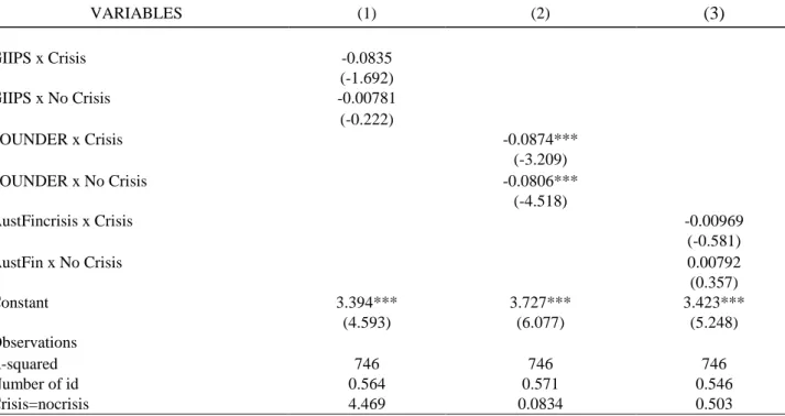
Table 4 – Impact of the Crisis in Different Groups (1985-2015)
VARIABLES (1) (2) (3) GIIPS x Crisis -0.0835 (-1.692) GIIPS x No Crisis -0.00781 (-0.222) FOUNDER x Crisis -0.0874*** (-3.209) FOUNDER x No Crisis -0.0806*** (-4.518) AustFincrisis x Crisis -0.00969 (-0.581) AustFin x No Crisis 0.00792 (0.357) Constant 3.394*** 3.727*** 3.423*** (4.593) (6.077) (5.248) Observations R-squared 746 746 746 Number of id 0.564 0.571 0.546 Crisis=nocrisis 4.469 0.0834 0.503
Note: Robust t-statistics in parentheses. *** denotes significance at 1%, ** at 5% and* at 10%. Year Dummies, constant and other control variables are not reported. The test of equivalence of coefficient is present in Crisis=nocrisis, for example in column (2) this value is 0.0834, meaning that we can reject that the two FOUNDER coefficients are different
18 So lastly, in table 4 we make regression like those in table 2, where each group considers a period before the crisis and after the euro introduction and another period after crisis, so in Table 4 we regress each group dividing it between the two periods. The FOUNDER coefficients are statistical significant in both Periods however when we test if the coefficients are statistically different the F-statistic is of 0.0834, so we reject that they are different, confirming that the euro impact in the FOUNDER group is across all period and furthermore that the crisis seems to not affect this countries as a group.
This leaves us with one last question, if the crisis affects the euro economies which group of countries are mostly affect by it? So now knowing that the euro has a significant impact on the FOUNDER real GDP per growth and that the euro area experienced lower growth during the period after 2010, in the following test we only consider these two variables and drop the dummy for the EA. So, crossing the Groups defined before with the dummy for the crisis (Table 5), we find that the GIIPS faced in fact a higher impact than the average during the crisis years (already in Table 4 we could see that both periods were statistically different), and when compared with the other groups crisis years it is the only that has a negative statistical coefficient. So, as we can see in column (7) in Table 5 when holding everything else constant, in crisis years on average GDP per head on the GIIPS countries decreases by 1,58%, per year, when compared to non-crisis years, however we cannot say that this effect is due to the presence of these economies in the euro.
19
Table 5- Effect of the crisis (1985-2015)
VARIABLES (1) (2) (3) (4) (5) (6) (7) (8) (9) FOUNDER -0.0718*** -0.0700*** -0.0738*** -0.0749*** -0.0669*** -0.0806*** -0.0781*** -0.0789*** -0.0783*** (-3.475) (-3.582) (-3.931) (-4.025) (-3.255) (-4.455) (-4.011) (-4.016) (-4.326) noFOUNDER -0.00479 (-0.145) crisis -0.0451* -0.0472* -0.0193 -0.0158 -0.0541* -0.0626* (-1.963) (-1.767) (-0.918) (-0.607) (-1.705) (-1.739) GIIPS x Crisis -0.0577 -0.0609 -0.0729* -0.0743* -0.0742* (-1.364) (-1.364) (-1.763) (-1.791) (-1.764) AustFin x Crisis -0.00797 0.0289 -0.0218 -0.0220 (-0.292) (0.883) (-1.001) (-0.978) FOUNDER x Crisis 0.0422 -0.00165 (1.113) (-0.0691) Constant 3.669*** 3.681*** 3.630*** 3.628*** 3.678*** 3.610*** 3.626*** 3.623*** 3.625*** (5.277) (5.658) (5.340) (5.327) (5.597) (5.305) (5.358) (5.333) (5.291) Observations 746 746 746 746 746 746 746 746 746 R-squared 0.579 0.579 0.584 0.584 0.580 0.581 0.583 0.583 0.583 Number of id 33 33 33 33 33 33 33 33 33
Year FE YES YES YES YES YES YES YES YES YES
Note: Robust t-statistics in parentheses. *** denotes significance at 1%, ** at 5% and* at 10%. Year Dummies, constant and other control variables are not reported..
20 5. Conclusion
The literature review leaved us with mixed feelings, at lead us to ask our first question: “Does adopting the euro affect Economic Growth?”. Second, literature often mentions struggle from part of the less developed countries of the south to impose their view in the decision making of the Euro Area leading us to ask if in fact the impact of the euro was the same for all countries. To address this question, we used a Fixed Effect model, that considers the OECD economies between 1985-2015, to explain GDP growth and used a dummy to control for the creation of the Euro.
Firstly, we found that either European Union or Euro Area membership have a significant impact on growth. At first, membership of the Euro Area seems to have a negative impact but when we controlled for the crisis after 2010 the effect becomes insignificant. When we look if the euro has differentiated impact, the results suggest so. The countries that founded the European Union experienced a lower growth across all the period of the euro´s functioning and that effect is not related with the crisis. This result is surprising, despite common knowledge this study suggests that indeed the euro harmed GDP growth in these economies.
We also found a negative impact of the crisis in the euro economies, nevertheless we were able to isolate that effect as being specific of the GIIPS economies. We cannot, however, infer that this result is because these countries are euro economies or, for example, that these countries bear most of the cost of the Sovereign Debt Countries ( Grauwe and Ji 2016). Our approach did not leave space to account for the impact of the new entries, leaving that effect to be explained out of our model.
Like other cross-country growth analysis our work is plagued with the problem of ambiguous choice of variables, as we use multiple variables to proxy what in fact we want to capture (Levine and Renelt 1992). Nevertheless, we use variables commonly used in growth regression therefore we believe that our conclusions remain valid. A 5-year approach using
21 lagged initial values and the fixed effect methodology mitigate the problems of endogeneity, at the same time the use of an OECD sample reduces other problem commonly present in growth regression that is parameters endogeneity.
Why do the FOUNDER groups grow less? Why do the GIIPS GDP growth is affected by the crisis? We are not able to answer these questions, nevertheless they are worth of future analysis.
22 References
Baldwin, Richard E. 1992. “Measurable Dynamic Gains from Trade.” Journal of Political
Economy 100 (1):162–74.
Barro, Robert. 1991. “Economic Growth in a Cross Section of Countries.” The Quarterly Journal
of Economics 106 (2):407–43.
Barro, Robert. 2013. “Education and Economic Growth.” Annals of Economics and Finance 14 (2):301–28.
Carkovic, Maria, and Ross E. Levine. 2002. “Does Foreign Direct Investment Accelerate Economic Growth?” SSRN Electronic Journal.
Checherita-Westphal, Cristina, and Philipp Rother. 2012. “The Impact of High Government Debt on Economic Growth and Its Channels: An Empirical Investigation for the Euro Area.”
European Economic Review 56 (7):1392–1405.
Easterly, William. 2005. “National Policies and Economic Growth: A Reappraisal.” In Handbook
of Economic Growth, edited by Philippe Aghion and Steven Durlauf, 1:1015–59. Handbook
of Economic Growth. Elsevier.
Freitas, Miguel Lebre de, Filipa Pereira, and Francisco Torres. 2003. “Convergence among EU Regions, 1990–2001: Quality of National Institutions and ‘Objective 1’ Status.”
Intereconomics 38 (5):270–75.
Glick, Reuven. 2016. “Currency Unions and Regional Trade Agreements: EMU and EU Effects on Trade.” Working Paper Series 2016–27. Federal Reserve Bank of San Francisco.
Glick, Reuven, and Andrew Rose. 2016. “Currency Unions and Trade: A Post-EMU Reassessment.” European Economic Review 87 (C):78–91.
Grauwe, PAUL DE. 2006. “What Have We Learnt about Monetary Integration since the Maastricht Treaty?*.” JCMS: Journal of Common Market Studies 44 (4):711–730.
23 Grauwe, Paul De, and Yuemei Ji. 2016. “Crisis Management and Economic Growth in the
Eurozone.” In After the Crisis, edited by Francesco Caselli, Mário Centeno, and José Tavares, 46–72. Oxford University Press.
KUNČIČ, ALJAŽ. 2014. “Institutional Quality Dataset.” Journal of Institutional Economics 10 (1):135–161.
Levine, Ross, and David Renelt. 1992. “A Sensitivity Analysis of Cross-Country Growth Regressions.” The American Economic Review 82 (4):942–63.
Mankiw, N. Gregory, David Romer, and David N. Weil. 1992. “A Contribution to the Empirics of Economic Growth*.” The Quarterly Journal of Economics 107 (2):407–37.
Mundell, Robert. 1961. “A Theory of Optimum Currency Areas.” The American Economic Review 51 (4):657–665.
Sachs, Jeffrey D., and Andrew M. Warner. 1995. “Natural Resource Abundance and Economic Growth.” Working Paper 5398. National Bureau of Economic Research.
Sachs, Jeffrey, and AM Warner. 1997. “Fundamental Sources of Long-Run Growth.” American
Economic Review 87:184–88.
Silva, J. M. C. Santos, and Silvana Tenreyro. 2010. “Currency Unions in Prospect and Retrospect.” CEP Discussion Papers dp0986. Centre for Economic Performance, LSE.
Solow, Robert. 1956. “A Contribution to the Theory of Economic Growth.” The Quarterly Journal
of Economics 70 (1):65–94.
Sousa, José de, and Julie Lochard. 2011. “Does the Single Currency Affect Foreign Direct Investment?*.” The Scandinavian Journal of Economics 113 (3):553–578.
Sachs, Jeffrey, and AM Warner. 1997. “Fundamental Sources of Long-Run Growth.” American
Economic Review 87:184–88.
Silva, J. M. C. Santos, and Silvana Tenreyro. 2010. “Currency Unions in Prospect and Retrospect.” CEP Discussion Papers dp0986. Centre for Economic Performance, LSE.