Faculdade de Engenharia da Universidade do Porto
Diagnosing Faults in Power Transformers With
Autoassociative Neural Networks and Mean Shift
Rafael Paiva Tavares
V
ERSÃOF
INALDissertação realizada no âmbito do
Mestrado Integrado em Engenharia Eletrotécnica e de Computadores
Major Energia
Orientador: Professor Vladimiro Miranda
Junho 2012
Resumo
Desde a Primeira Guerra Mundial que o diagnóstico de transformadores de potência é uma preocupação dos fabricantes e empresas do sector elétrico.
Por isso, vários métodos de diagnóstico foram propostos ao longo do tempo, sendo um dos mais conhecidos e utilizados o método de análise dos gases dissolvidos no óleo do transformador.
Hoje em dia, com a crise económica, a possibilidade de reduzir o custo de manutenção e também os custos de aquisição de novas máquinas é do agrado de todas as empresas do setor energético. Esta redução de custos permite que estas empresas tenham a possibilidade de reduzir o custo final da energia para o consumidor final, algo que é de extrema importância.
Nesta tese, vários métodos de diagnóstico utilizando o princípio da análise dos gases dissolvidos no óleo e diferentes ferramentas matemáticas são desenvolvidos e testados.
Devido aos dados disponíveis serem poucos, recorreu-se ao algoritmo de Mean Shift com o objetivo de criar dados virtuais para treinar as redes neuronais, sendo os dados reais utilizados apenas para o processo de validação do treino.
Palavras-chave: transformadores de potência, diagnóstico de avarias, análise de gases
Abstract
Diagnosing power transformers as been since at least the First World War, a concern of both utilities and machine manufacturers. Therefore, several methods were proposed, being one of the most known the Dissolved Gas Analysis method.
Nowadays, with the economical crisis, the possibility to save money in maintenance and in the acquisition of new machines pleases the utilities. These savings also allow selling energy at a lower cost to the final consumer, being this one of the utilities objective.
In this thesis, several diagnosis methods are developed and tested, using different mathematical tools and the Dissolved Gas Analysis method principle.
Because of the sparse data, Information Theoretic Learning Mean Shift algorithm is used in order to create virtual points to train neural networks, leaving the real data only to its validation.
Keywords: Power transformers, fault diagnosis, dissolved gas analysis, autoassociative neural
Acknowledgements
First of all, I would like to present my most sincere ‘Thank You’ to my parents. They were the most supportive people in the last five years. I also know that financially supporting a kid living away from home during five years is a pretty hard task and I love you for that effort.
To my brother, with whom I shared a house again in the last two years, I know putting up with me can be a hard task, but you accomplished it well.
I also know that, in the last four or five months I have been impatient, bad-humoured and a stressed guy, but my girlfriend never showed the least sign of being tired of me. For that, I must thank you.
To all my friends who also had to deal with me in a regular basis, I admire your patience. A very special thanks needs to go EFACEC, a Portuguese power transformer manufacturer, and to Eng. Jácomo Ramos as General Manager – Technology, for the interest in cooperating with this thesis work and authorizing the use of EFACEC’s data. A warm and kind word is addressed to Dr. Maria Cristina Ferreira who was always extremely supportive and with generous availability to help me.
A very kind word needs to go to Professor Vladimiro Miranda. Most of the ideas in this thesis are his.
Table of Contents
Resumo ... III
Abstract ... V
Acknowledgements ... VII
Tables Index ... XIII
Abbreviations and symbols ... XIV
Abbreviations list: ... XIV
Symbols list ... XIV
Chapter 1. Introduction ... 1
Chapter 2. State of the Art ... 3
2.1. Dissolved Gas Analysis ... 3
2.1.1. IEC60599 Standard ... 4
2.1.2. IEEE Guide for the Interpretation of Gases Generated in Oil-‐Immersed
Transformers ... 5
2.1.3. Other methods ... 6
2.1.4. Alternatives offered in the market ... 8
2.2. Kernel density estimation ... 9
2.3. Mean shift algorithm ... 10
2.3.1. Iterative algorithm ... 12
2.3.2. Steepest descent algorithm ... 12
2.4. Autoassociative neural networks ... 14
Chapter 3. Densification of data sets ... 15
3.1. The database ... 15
3.2. Information Theoretic Learning Mean Shift algorithm applications ... 16
3.2.1. Using the ITLMS as a mode seeking tool ... 16
3.2.2. Densification trick using ITLMS ... 20
3.2.1. Other ITLMS applications ... 24
Chapter 4. Incipient fault diagnosis systems ... 27
4.1. A diagnosis system using autoencoders ... 27
4.2. Diagnosis using neural networks with binary outputs ... 32
4.3. Mean absolute error and modes method ... 38
4.4. Steepest Descent and mean absolute error method ... 40
4.5. Method Comparison ... 43
Chapter 5. New Industrial Data ... 45
Chapter 6. Robustness tests ... 49
6.1. Introduction ... 49
6.2. Autoencoders method ... 51
6.3. Neural networks with binary outputs method ... 54
Chapter 8. Suggestions of work to do in the future ... 59
References ... 61
Appendixes ... 65
Appendix A – ITLMS cluster features seeking ... 65
Appendix A.1 – Modes seeking (λ = 1, σ = mean (std)) ... 65
A.3 – Local modes seeking (λ = 1, σ = various) ... 73
A.4 – Finer cluster structures seeking (λ = 7, σ = various) ... 77
Appendix B – Densification trick ... 81
B.1 – Using λ = 1, σ = mean (std) ... 81
Appendix C – Paper “Discovering structures in DGA clusters with applications in
several methods for fault diagnosis” ... 85
Figures Index
Figure 2.1 - IEC60599 graphical representation of gas ratios [2] ... 5
Figure 2.2 - Example of a possible autoencoder architecture ... 14
Figure 3.1 - Low-energy cluster fault ITLMS mode seeking output σ = mean (std) ... 17
Figure 3.2 - Low-energy fault cluster ITLMS mode seeking output σ = 0.5*mean (std) ... 18
Figure 3.3 - Database mode seeking output using ITLMS (σ = 0,35*meanstd) ... 19
Figure 3.4- Low-energy discharge ITLMS consecutive application (λ = 1, σ = mean (std)) ... 21
Figure 3.5 - Low-energy discharge fault ITMLS consecutive application (λ = 2, σ = mean (std)) .... 22
Figure 3.6– Thermal fault (T>700ºC) ITMLS finer structures seeking (λ = 7, σ = 0,75*mean (std)) ... 24
Figure 3.7 – Low-energy discharge fault ITLMS local modes seeking output (λ = 1 , σ = 0,5*mean (std)) ... 25
Figure 4.4.1 - Autoencoders diagnosys system architecture ... 28
Figure 4.2 - Partial discharge autoencoders diagnosys error comparison ... 29
Figure 4.3 - Low-energy discharge autoencoders diagnosys error comparison ... 30
Table 4.1 – Autoencoder method results summary ... 31
Figure 4.4 - Binary neural networks diagnosys system architecture ... 33
Figure 4.5 - Partial discharge binary neural networks error comparison ... 34
Figure 4.6 - Low-energy discharge binary neural networks error comparison ... 35
Figure 4.7 - High-energy discharge binary neural networks error comparison ... 36
Figure 4.8 - Healthy state of transformers with OLTC binary neural networks error comparison .... 37
Figure 4.9 - mean absolute error and modes method architecture ... 38
Figure 4.10 - Steepest descent and mean absolute error method architecture ... 40
Figure 5.1 - Number of correct diagnoses of EFACEC data by method ... 47
Figure 6.1 - Robustness tests algorithm ... 49
Figure 6.1a - Robustness testes to autoencoders method results ... 51
Figure 6.1b - Robustness testes to autoencoders method results ... 52
Figure 6.2a - Robustness tests to binary neural network method results ... 54
Figure 6.2b - Robustness tests to binary neural network method results ... 55
Figure A.1.1 – Low-energy discharge modes seeking ... 65
Figure A.1.2 – High-energy discharge modes seeking ... 65
Figure A.1.3 – Partial discharge modes seeking ... 66
Figure A.1.4 – Thermal fault (T<700ºC) modes seeking ... 66
Figure A.1.5 – Thermal fault (T>700ºC) modes seeking ... 67
Figure A.1.6 – Healthy transformer without OLTC modes seeking ... 67
Figure A.1.7 – Healthy transformer with OLTC modes seeking ... 68
Figure A.2.1 – Low-energy discharge principal curve seeking ... 69
Figure A.2.2 – High-energy discharge principal curve seeking ... 69
Figure A.2.3 – Partial discharge principal curve seeking ... 70
Figure A.2.4 – Thermal fault (T<700ºC) principal curve seeking ... 70
Figure A.2.5– Thermal fault (T>700ºC) principal curve seeking ... 71
Figure A.2.6 – Healthy transformer without OLTC principal curve seeking ... 71
Figure A.2.6 – Healthy transformer with OLTC principal curve seeking ... 72
Figure A.3.3 – Partial discharge local modes seeking ... 74
Figure A.3.4 – Thermal fault (T<700ºC) local modes seeking ... 74
Figure A.3.5 – Thermal fault (T>700ºC) local modes seeking ... 75
Figure A.3.6 – Healthy transformers without OLTC local modes seeking ... 75
Figure A.3.7 – Healthy transformers with OLTC local modes seeking ... 76
Figure A.4.1 – Low-energy discharge finer structures seeking ... 77
Figure A.4.2 – Low-energy discharge finer structures seeking ... 77
Figure A.4.3 - Partial discharge finer structures seeking ... 78
Figure A.4.4 – Thermal fault (T<700ºC) finer structures seeking ... 78
Figure A.4.5 – Thermal fault (T>700ºC) finer structures seeking ... 79
Figure A.4.6– Healthy transformer without OLTC finer structures seeking ... 79
Figure A.4.7– Healthy transformer with OLTC finer structures seeking ... 80
Figure B.1.1 – Low-energy discharge densification trick (λ = 1, σ = mean (std)) ... 81
Figure B.1.2 – Low-energy discharge densification trick (λ = 1, σ = mean (std)) ... 81
Figure B.1.3 – Partial discharge densification trick (λ = 1, σ = mean (std)) ... 82
Figure B.1.4 – Thermal fault (T<700ºC) densification trick (λ = 1, σ = mean (std)) ... 82
Figure B.1.5 – Thermal fault (T>700ºC) densification trick (λ = 1, σ = mean (std)) ... 83
Figure B.1.6 – Healthy transformer without OLTC densification trick (λ = 1, σ = mean (std)) ... 83
Tables Index
Table 2.1 - IEC60599 gas ratio intervals [2] ... 4
Table 2.2 – Data, results and comments of distinct systems / publications [1] ... 7
Table 3.1 - Number of real cases per fault in the database ... 15
Table 3.2 - Database complete description (using λ = 1 and σ = mean(std) ... 23
Table 4.1 – Autoencoder method results summary ... 31
Table 4.2 – results obtained with MAE and modes method summary ... 39
Table 4.3 - Steepest descent and MAE method results (when recognising only faulty states) (ITLMS data created with λ = 1 and σ = meanstd) ... 41
Table 4.4 - Steepest descent and MAE method results (when recognising seven healthy/faulty states) ... 41
Table 4.5 - Diagnosis methods comparison ... 43
Abbreviations and symbols
Abbreviations list:
ANN Artificial Neural Network DGA Dissolved Gas Analysis DH High-energy Discharge DL Low-energy Discharge GBMS Gaussian Blurring Mean Shift GMS Gaussian Mean Shift
IEC International Electrotechnical Commission ITLMS Information Theoretic Learning Mean Shift MAE Mean Absolut Error
OLTC On Load Tap Changer PD Partial Discharge
pdf Probability Density Function std Sandard Deviation
T1 Thermal Fault 150ºC<T<300ºC T2 Thermal Fault 300ºC<T<700ºC T3 Thermal Fault T>700ºC TC Technical Committee
TDCG Total Dissolved Combustible Gas UFPA Universidade Federal do Pará
Symbols list
C Carbon CO Carbon monoxide 𝐶!𝐻! Acetylene 𝐶!𝐻! Ethylene 𝐶𝐻! Methane 𝐶!𝐻! Ethane H Hydrogen (radical) 𝐻! Hydrogen (molecular) T Temperature ºC Celsius degrees 𝜆 Lagrange MultiplierChapter 1.
Introduction
A power transformer is an electric machine generally used to change the voltage level in an electric power system.
Power transformers are a key component in any electric system. They are very expensive machines and, when there is a severe fault, the consequences can affect not only the machine itself but also surrounding facilities, equipment and people. Replacing or repairing a power transform, besides being very expensive, can also take a lot of time, which can make the consequences even worse. There are thousands of these machines in any generation, transmission and distribution system; therefore, their reliability is extremely important to maximize the energy sold and the global effectiveness and efficiency of the electric system.
Thus, any tool that can prevent a transformer to go out of service, minimize its repair cost or prevent accidents is very important and useful to utilities and transformer manufacturers.
It is known that when a fault occurs inside a power transformer, in its initial state, the consequences are very small, allowing the machine to work, and can be neglected. However, as time passes, those small faults can evolve to a more severe state that may not be reparable or may lead to the destruction of the machine. The main goal of any diagnosis system is to detect faults in their initial state and identify which type of fault occurred, if any. This allows the machine owner to analyse the situation and take preventive and corrective measures to maximize the power transformer lifetime. It is also important that these diagnosis methods can be applied while the machine is kept in service, because its disconnection may be very expensive and last for a long time. This latter point is related to the costs of the non-supplied energy.
This thesis has as main objective the studying, building and testing of new methods to diagnose power transformers. All these methods are based on the Dissolved Gas Analysis technique and the use of gas concentration ratios. Some other mathematic tools used are the Information Theoretic Mean Shift algorithm – ITLMS and neural networks, mainly a special kind of these networks often called auto associative neural networks or just autoencoders.
All these concepts and tools will be explained in following chapters of this document. It should be noticed that this work continues what has already been published in [1]. To develop this thesis, the most used software was the MATLAB R2011b version from Mathworks.
Chapter 2.
State of the Art
2.1. Dissolved Gas Analysis
The dissolved gases in power transformer oil are known to contain information about the condition of the machine. Utilities and manufacturers have been using this tool for several decades, since the First World War, to diagnose power transformers using a technique called Dissolved Gas Analysis (DGA) [1].
The power transformer oil is often mineral. Its role is insulation, thermic energy dissipation and constituting a dielectric environment. Since an oil sample can be retrieved without turning off the machine, a DGA technique allows diagnosing the condition of a power transformer at any time. This allows maximizing the power system reliability and maintenance scheduling before a small fault (incipient fault) evolves to a more severe state, like a non-reparable one. Because of this aptitude to expand the lifetime of power transformers, DGA has been recognized as such a powerful tool that, nowadays, is a standard to the electric industry worldwide.
The typical oil chemical composition is a mix of hydrocarbon molecules. Those are linked together with carbon-carbon and carbon-hydrogen bounds that can be disrupted by thermic or electric faults. When this occurs, some ions come free and recombine with other molecules, adding new chemical elements to the oil. Therefore, with machine usage and its consequent material and component degradation, the oil absorbs the gases released. This allows the inspection of the transformer condition. [2]
Different chemical compounds are created when the energy released by the fault varies, since low energy faults break the C-H bound, because they are weaker, while faults with higher energy break the C-C bounds. This means that the different gas concentrations provide information about the type of fault and its severity.
There are a lot of DGA methods using a mix of mathematic tools and different indicators. Single gas concentrations and total volume of gas in oil can be used, however there is also a key gas method, where each fault is related with one gas concentration or, the most used technique, which applies gas ratios to diagnose the transformer. In this last method there are two different techniques, the Doernenburg ratio method and the Rogers ratio method. Even though they follow
Chapter 2. State of the Art
Some methods like the International Standard IEC60599 set boundaries to gas concentration in order to classify different faults. To account for the limitations of rigid boundary definition, fuzzy set approaches have been proposed [5, 6]. The results achieved by these systems are promising, however the tuning process of the diagnosis rules may be difficult to handle. Because of the superior learning ability and the built-in power to handle data with error, Artificial Neural Networks (ANNs) have been used in DGA. These systems can be in continuous learning with new samples. However, the neural network training is often a slow process because it is sensitive to local minima presence and the backpropagation methods have trouble in dealing with this feature. [7]
2.1.1. IEC60599 Standard
The international standard IEC60599 - Mineral oil-impregnated electrical equipment in service – Guide to the interpretation of dissolved and free gases analysis [2, 8], is a milestone in the DGA methods. The last version of this document was released in 1999 and distinguishes six different faults:
• Partial Discharges (PD) • Low Energy Discharges (D1) • High Energy Discharges (D2) • Thermal Faults, T<300ºC (T1) • Thermal Faults, 300ºC<T<700ºC (T2) • Thermal Faults, T>700ºC (T3) And defines them as
• Partial Discharge – electric discharge where only a small part of the insulation is bridged with small perforations
• Discharge – electric discharge with total insulation bridge through carbonization (low energy discharge) and metal fusion (high energy discharge)
• Thermal fault – excessive temperature in the insulation. This fault can turn the insulation (T<300ºC), carbonize it (300ºC<T<700ºC), melt the metal and carbonize the oil (T>700ºC). This publication assumes that every fault can be diagnosed using three gas ratios:
!!!! !!!!
!!! !!
!!!! !!!! where: 𝐶!𝐻! is acetylene 𝐶!𝐻! is ethylene 𝐶𝐻! is methane 𝐻! is hydrogen 𝐶!𝐻! is ethane
As said before, this standard sets intervals to these ratios, as shown in the table 2.1: Table 2.1 - IEC60599 gas ratio intervals [2]
Fault 𝐶𝐶!𝐻! !𝐻! 𝐶𝐻! 𝐻! 𝐶!𝐻! 𝐶!𝐻! PD - <0,1 <0,2 D1 >1 0,1 - 0,5 >1 D2 0,6 - 2,5 0,1 - 1 >2 T1 - - <1 T2 <0,1 >1 1 – 4 T3 <0,2 <1 >4
2.1 - Dissolved Gas Analysis
This way, the space is divided in parallelepipeds as can be seen in figure 2.1:
Figure 2.1 - IEC60599 graphical representation of gas ratios [2]
This standard also states that gas ratios should only be calculated if any of the gas concentrations is larger than the typical healthy values or the rate of gas increase is larger than the usual values, also published.
In addition to these faults, three more gas ratios are introduced: !!!! !!
;
!! !!;
!!! !";
where the first one is related with the possibility of contamination of the OLTC compartment, the second one with an unusual heating of the gas and the third one with the cellulose degradation.
Diagnosing power transformers using this method has 93,94% of correct diagnoses [1].
2.1.2. IEEE Guide for the Interpretation of Gases Generated in Oil-Immersed Transformers The IEEE published a guideline paper in power transformers diagnosis, the IEEE Guide for the Interpretation of Gases Generated in Oil-Immersed Transformers [3]. Its scope is very similar to the IEC standard, however the diagnosis according to this publication can be done in several ways: using individual and total dissolved combustible gas analysis (TDCG), by the key gas method and Doernenburg and Rogers ratios methods.
The first method defines sampling time intervals and operation procedures that depend of TDCG increase per day and TDCG value.
The key gas method uses the larger gas concentration in the oil to diagnose the machine. For example, when larges quantities of CO (carbon monoxide) are found in the transformers oil, this method diagnoses this fault as a thermal one.
Chapter 2. State of the Art
As said before, the Doernenburg and Rogers method are very similar, however they differ in the ratios used. While the Doernenburg method uses five gas ratios, the Rogers method uses only three, not considering the Hydrogen concentration to diagnose the machine.
The Rogers method is the most similar to the IEC method because the number of ratios (and two of these) are the same, however one of them and the number of faults diagnosed differ, with the IEC method recognizing one more fault.
2.1.3. Other methods
Beside the two standards referred to above, there are other methods to diagnose power transformers using a DGA technique and several mathematical tools. These methods were developed before the publication of the standards and were used as basis to them or were developed after those milestones in order to improve the results of diagnosis made using these standards.
There are methods that use artificial neural networks and hybrid fuzzy sets [9, 10], expert systems [11], Support Vector Machines [12], self-organizing maps or Kohonen neural networks [13], fuzzy set models [14], wavelet networks [15], radial basis function neural network [6], multi-layer feedforward artificial neural networks [7, 16].
One of those methods was published by Wang et all in [11]. In this method a combined expert system and neural network is used. This way, the advantages of neural networks are combined with the human expertise.
In 1999, Yang et all [5], published a paper suggesting the use of an adaptive fuzzy system to diagnose power transformers. The system was presented as a self-learning one, using also the rules of the Doernenburg.
Other method using neural networks was published by Zhang in [16]. This method, even though a single neural network is used to diagnose the major fault types; it is also used an independent neural network to diagnose the cellulose condition.
Huang, in [7], also proposed the use of neural networks to diagnose power transformers. However, to train these neural nets an evolutionary algorithm is used. This way, the optimal connection weights and bias can be found easily and the disadvantages of the steepest-decent method are avoided.
In order to make explicit the implicit knowledge stored in neural networks after the training, Castro et al. published in [17] an algorithm to transform a neural network black box action in a set of explicit rules. After that, this method was applied in a power transformer diagnosis method.
In [1], Shigeaki suggests the use of seven autoencoders that work in parallel, that is, in a competitive way. This method will be explained later in this thesis because it will be used. In the following table, one can find a summary of all methods referred here, as well as some others methods and the corresponding results. This table is the one below (Table 2.2):
2.1 - Dissolved Gas Analysis
Table 2.2 – Data, results and comments of distinct systems / publications [1]
Model Year
No. Samples % of correct diagnoses No.
Faults Comments Total Test Training Test
Y Zhang et
al [16] 1996 40 ? ? 95 3+N
ANN. Too few testing samples: presumed only 2-3 testing samples on average per mode. Wang [11] 1998 188+22 60 99,3 to 100 93,3 to 96,7 5+N combined. No PD fault mode. Expert System and ANN
YC Huang
et al [7] 2003 220+600 0 95,12 -- 4+N
ANN modified by Evolutionary Algorithm. No validation. Only 220 samples for fault cases, 600
for normal state. HT Yang,
CC Lao [5] 1999 561 280 93,88 94,9 4+N
Fuzzy rule system. Use of additional 150 artificial data for
3 extra types of faults. Guardado
et al [18] 2001 69 33 100 100 5+N
ANN trained with 5 gas ppm concentrations. Too few testing samples: only 5 testing samples
av. Per mode. Castro,
Miranda
[17] 2005 431 139 100 97,8 3
ANN and fuzzy rule system. No normal mode. Includes IEC TC10
data. Miranda,
Castro [9] 2005 318 88 100 99,4 5
ANN and fuzzy rule system. IEC TC10 data. No normal
mode.
G LV et al
[19] 2005 75 25 100 100 3+N
3 cascading SVMs. Data for 1 single transformer and not from
a diversity of machines. Too few testing samples: only 2 samples for testing DH faults. WH Tang
et al [20] 2008 168 ? ? 80 3+N
Applies Parzen windows and PSO.
LX Dong et
al [21] 2008 220 60 ? 88,3 3+N
Applies a rough set classifier and the fusion of 7 wavelet neural networks. No PD mode.
MH Wang
et al [22] 2009 21 0 100 -- 8+N
Couples the Extension Fuzzy Set theory with Genetic algorithms. No validation. Too few samples: only 2 testing samples on av.
per mode. SW Fei,
XB, Zhang
[23] 2009 142 ? ? 94,2 3+N
Apples cascading SVM tuned with a Genetic Algorithm. No PD
mode. No information on the size of test set, presumed
small. NAM Isa et
al [24] 2011 160 40 100 100 3+N
Couples a feed-forward neural network with k-mean
clustering. Castro,
Miranda
[1] [25] 2011 318 88 100 100 5
Autoencoders. No normal mode. Small number of test samples in
some modes. K Bacha et
al [26] 2012 94 30 ? 90 6+N
Applies SVM. Too few samples: PD mode with only 2 samples, DL mode with only 3 samples,
Chapter 2. State of the Art
When analysing the table above, one must take into account that different data sets were used in all the methods. Therefore, a comparison between the methods must be done carefully. Nevertheless, this table gives an idea how each method behaves when diagnosing a power transformer.
2.1.4. Alternatives offered in the market
Since dissolved gas analysis is an industrial standard to diagnose power transformers, there are several companies that provide this service. These companies can be power transformers manufacturers that supply their costumers with the possibility of, as a regular procedure, analyse the transformers’ oil to allow early problem detection. This is the most usual approach do analyse the gas concentrations dissolved in oil and is done by companies like EFACEC. However there are monitoring systems that can be installed in the power transformer itself in order to maintain a continuous surveillance of the machine health state. This way, there is no need to periodically get an oil sample to analyse because this is done online and in situ. Companies like SIEMENS offer this service to costumers [27].
There are also companies that don’t produce transformers but sell diagnosis of power transformers to its owners even though the manufacturers offer this service. Some examples are DOBLE Engineering [28] and POWERTECH Labs [29].
Almost all of these companies make use of one or a mix of both of the standard described before, however, they make small changes based in know-how acquired with experience. Usually these changes are made in the gas concentrations limits or the ratios values. In spite of this, there are companies who have also developed their own diagnosis methods or complemented the standards with more analysis like the dissolved metals in oil.
2.2 - Kernel density estimation
2.2. Kernel density estimation
Knowing that the probability 𝑃 of a vector 𝑦 fall in a region 𝛩 is given by: 𝑃 = 𝑝 𝑥! 𝜕𝑥′
! ( 2.1 )
it is possible to estimate a smoothed version of 𝑝 estimating the value of the probability 𝑃 [30]. Kernel density estimation, namely the Parzen window technique [31], is a popular non-parametric method for estimating the probability density function of a data set [32]. The idea behind this estimation is very simple: placing a kernel over the samples and interpolating, with the proper normalization, gives the density estimation in each point. Therefore, the contribution of each sample in the estimation of the pdf is done in accordance to its distance to the point where the kernel is centred. If this is done to all the data set, one is able to estimate the complete pdf.
The kernel density estimation for a point of the data set in a d-dimensional space is given by:
𝒑 𝒙, 𝝈 =𝟏 𝑵 𝑮 𝒙 − 𝒙𝒊 𝝈 𝟐 𝑵 𝒊!𝟏 ( 2.2 )
where G is the kernel, 𝜎 is the kernel bandwidth and N is the number of data points.
The kernel bandwidth has serious implications in the results given by this method. When 𝜎 is large, the closest samples have a very small weight, therefore, it is assumed that the pdf is a smooth, slowly changing function and the result will be a function with little resolution. On the other hand, when 𝜎 is smaller, the resulting pdf is a noisy one, with peaks centred in the samples. In this case the resolution is bigger, however, it can be affected by statistical variability. This way, one needs to seek some compromise between both cases [30, 33].
The estimation of the probability density function is a very useful mathematical tool to deal with discrete data sets because it allows transforming them in a continuous probability density function.
Chapter 2. State of the Art
2.3. Mean shift algorithm
The Mean Shift algorithm is a mathematic formulation that allows analysing arbitrarily structured feature spaces. It can be used to find the modes or the principal curves of the datasets. In this algorithm the dataset is represented by its probability density function, where the modes can be found in the maximum of this function. It is a very versatile and robust algorithm in feature space analysis [32] and is often used in image segmentation [34, 35], denoising, tracking objects [36] and a several other computer vision tasks [37, 38].
Fukunaga and Hostler firstly introduced a Mean Shift algorithm in 1975 [39]. In this paper they showed that this algorithm is a steepest descent technique where the points of a new dataset are moving in each iteration towards the modes of the original dataset.
This first version of mean shift algorithm says that, if we consider a dataset 𝑋!= (𝑋!)!!!! ∈ 𝑅!,
using a Gaussian kernel given by 𝐺(𝑡) = 𝑒!!! and the Parzen window technique, we are able to
estimate the probability density function using:
𝒑 𝒙, 𝝈 =𝟏 𝑵 𝑮 𝒙 − 𝒙𝒊 𝝈 𝟐 𝑵 𝒊!𝟏 ( 2.3 ) where 𝜎 is the kernel bandwidth that is always bigger than 0. As mentioned before, the objective of this algorithm is to find the modes of the dataset where ∇𝑝 𝑥 = 0. With that in mind, the iterative fixed-point equation is:
𝑚 𝑥 = 𝐺 𝑥 − 𝑥! 𝜎 ! 𝑥! ! !!! 𝐺 𝑥 − 𝑥! 𝜎 ! ! !!! ( 2.4 )
The difference 𝑚 𝑥 − 𝑥 is known as mean shift.
This algorithm is known as Gaussian Blurring Mean Shift (GBMS) and it is unstable because the actual solution is a single point that minimizes the overall entropy of the data set – therefore, the modes cannot be confidently discovered.
In spite of this important development, the Mean Shift idea was forgotten until 1995, when Yizong Cheng [40] introduced a small change in the algorithm. While in Fukunaga’s algorithm the original dataset is forgotten after the first iteration, 𝑋(!)= 𝑋
!, Cheng algorithm keeps this dataset
in memory. This initial dataset is used in every iteration to be compared with the new dataset Y. However Y is initialized the same way, 𝑌(!)= 𝑋
!. This also introduces a small change in the
iterative equation: 𝑚 𝑥 = 𝐺 𝑥 − 𝑥!! 𝜎 ! 𝑥!! ! !!! 𝐺 𝑥 − 𝑥!! 𝜎 ! ! !!! ( 2.5 )
In literature, Fukunaga’s algorithm is known as Gaussian Mean Shift Algorithm (GMS).
In 2006, Sudhir Rao, Jose C. Principe and Allan de Medeiros Martins [41-43] introduced a new formulation of mean shift known as Information Theoretic Mean Shift (ITLMS) and showed that GBMS and GMS are special cases of this one.
The idea in this algorithm was to create a cost function that minimizes the cross entropy of the data while the Cauchy-Schwartz distance is kept at a given value.
2.3 - Mean shift algorithm
𝐺!= 𝑒 !!!
!!! ( 2.6 )
an estimation of a probability density function (pdf), using the Parzen window technique, is: 𝑝 𝑥 = 1
𝑁 𝐺! 𝑥 − 𝑥𝑖 !
!!!
( 2.7 ) Renyi’s quadratic entropy of a probability density function can be calculated using:
𝐻 𝑥 = − log !!𝑝! 𝑥 𝑑𝑥 !! ( 2.8 ) So, 𝐻 𝑥 = −log 1 𝑁! 𝐺!! 𝑥 − 𝑥! ! !!! ! !!! ( 2.9 ) where 𝜎!= 2𝜎.
In the literature, 𝐻 𝑥 is known as the information potential of a probability density function. This name was given because 𝐻 𝑥 resembles a potential field and its derivative reminds of forces between particles in physics. Hence, the derivate of 𝐻 𝑥 in each point gives the information force.
To measure the cross entropy between two pdf, one has: 𝐻 𝑥, 𝑥! = − log 𝑉 𝑥, 𝑥! = −log 1 𝑁! 𝐺!! 𝑥!− 𝑥!! ! !!! ! !!! ( 2.10 ) The Cauchy-Schwartz distance can be calculated using:
𝐷!" 𝑥, 𝑥!! = log
𝑝! 𝑥 𝑑𝑥 . 𝑞! 𝑥 𝑑𝑥
𝑝 𝑥 𝑞(𝑥)𝑑𝑥 ( 2.11 )
where 𝑝 and 𝑞 are pdfs.
Using all the definitions above, it is possible to formulate a cost function to minimize the cross entropy between the two pdfs while keeping the Cauchy-Schwartz distance at a value k:
F x = min𝐻 𝑥 𝑎𝑛𝑑 𝐷!" 𝑥, 𝑥! = 𝑘 ( 2.12 )
Using a Lagrange multiplier to transform a constrained cost function in an unconstrained one: F x = min 𝐻 𝑥 + 𝜆 𝐷!" 𝑥, 𝑥! − 𝑘 ( 2.13 )
and differentiating at each point: 𝑑𝐹 𝑑𝑥!= 𝑥! !!!=𝑐!∗ 𝑆!+ 𝑐!∗ 𝑆! 𝑐!∗ 𝑆!+ 𝑐!∗ 𝑆! ( 2.14 ) where: 𝑐!=1 − 𝜆 𝑉(𝑥) , 𝑐!= 1 − 𝜆 𝑉(𝑥, 𝑥0) ( 2.15 ) and:
Chapter 2. State of the Art 𝑆!= 𝐺! 𝑥!!− 𝑥 !! ! 𝜎′ ! !!! ∗ 𝑥!! ( 2.16 ) 𝑆!= 𝐺! 𝑥!!− 𝑥 !!! ! 𝜎′ ! !!! ∗ 𝑥!! ( 2.17 ) 𝑆!= 𝐺! 𝑥! !− 𝑥 !! ! 𝜎′ ! !!! ( 2.18 ) 𝑆!= 𝐺! 𝑥!!− 𝑥 !!! ! 𝜎′ ! !!! ( 2.19 )
As shown by Sudhir Rao, Weifeng Liu, Jose C. Principe and Allan de Medeiros Martins, adjusting the 𝜆 parameter changes the data properties sought by the algorithm:
• When 𝜆=0 the algorithm minimizes the data entropy, returning a single point. This is the GBMS algorithm.
• When 𝜆=1, the algorithm is a mode seeking method, the same as GMS.
• When 𝜆>1, the principal curve of the data is returned (1<𝜆<2). A higher value of 𝜆 makes the algorithm seek to represent all the characteristics of the pdf.
2.3.1. Iterative algorithm
With Rao’s formula for 𝑥!!!!, it is possible to build an iterative algorithm where each point of
the data set ‘travels’ in the data domain until it reaches a stable point where the information force is zero. This is the solution of the method and it can be a mode or a point that belongs to the principal curve of the data, depending on which value of 𝜆 is been used.
To stop this algorithm, the simplest way, is to calculate the distance (𝑑) between the points given in 𝑡 and 𝑡 + 1 iterations and interrupt the algorithm when 𝑑 is smaller than a tol level for 𝑘 consecutive iterations.
2.3.2. Steepest descent algorithm
Another way to build a mean shift algorithm is to apply the rules of steepest descent algorithms, building the equation 2.20:
𝑥!!!!= 𝑥 !!+ 𝜂
𝑑
𝑑𝑥!𝐽(𝑥) ( 2.20 )
In this case 𝐽(𝑥) is the formula of the unconstrained optimization problem that can be obtained using a Lagrange multiplier:
𝐽 𝑥 = min 𝐻 𝑥 − 𝜆(𝐷!" 𝑥, 𝑥! − 𝑘) ( 2.21 )
Differentiating 𝐽(𝑥):
𝑑
2.3 - Mean shift algorithm
Using this technique, one is able to adjust the 𝜂 parameter in the equation 2.20, which is the step of the iteration. With this capability it is possible to control how the points travel in the data’s domain, slower or faster, and the direction of the movement.
Chapter 2. State of the Art
2.4. Autoassociative neural networks
Autoassociative neural networks or just autoencoders are a subtype of feedforward neural networks. These are built and trained in such way that the output vector is the same, or almost the same, as the input vector. In other words, autoencoders work as recognition machines. Since the target output vector is equal to the input vector, the number of output and input neurons is always the same. In the simplest autoencoders, there is but one hidden layer however there can be more. This inner layer usually has a smaller number of neurons than the output and input layers, however it does not need to be always like that. When the hidden layer has a smaller number of neurons, called a bottleneck, the data is compressed between the input and hidden layers and decompressed between the hidden layer and the output layer, since the vector’s size is change to a smaller one. This kind of neural network is often used to compress data [44-47], restore missing sensor information [48, 49] and several other tasks [50, 51].
One interesting property of autoencoders is that when the network is trained to recognize a pattern, if an input vector with different characteristics is shown to the network, the error between the output and input tends to be high. This is extremely useful in pattern recognition tasks as detecting and restoration missing sensor information [52] and it is very important to the work done in this thesis.
Training an autoencoder is, in everything, similar to training any other neural network. The most used method to do it is known as backpropagation algorithm. In this algorithm the connection weights are adjusted in order to minimize a cost function, usually the minimum square error between the input and output vectors [53]. To train a neural network, two independent data sets are needed: one to train the network and other to validate its results. While the training set is used to adjust de connection weights, the validation set is used to verify if the network is generalising in a proper way. Generalising is the neural network ability to recognize points with the same properties of the ones in the training set but that didn’t belong to it.
Below, in the figure 2.2, a diagram showing the typical autoencoder architecture is shown:
Chapter 3.
Densification of data sets
3.1. The database
To proceed with the study, was used a database containing actual dissolved gas analysis data and the corresponding diagnoses. It is a compilation of data from the IEC TC10 database and from several other origins and it was kindly provided by Prof. Adriana Castro from UFPA.
The real cases database consists in:
Table 3.1 - Number of real cases per fault in the database
Case Fault/State samples No. of
PD Partial Discharge 30
DH High Energy Discharge 103
DL Low energy Discharge 37
T1 Thermal Fault (T<700ºC) 77 T2 Thermal Fault (T>700ºC) 71 OK Healthy State without OLTC 20 OK with OLTC Healthy State with OLTC 10
Total: 348
These seven faulty/healthy states shown in table 3.1 are the ones that all the diagnosis methods studied in this thesis are built to distinguish. That is the reason why there are always seven neural networks in the systems with neural networks.
When the three gas concentration ratios are calculated, some modifications are made in order to normalize the data: ratios impossible to calculate because infinite is returned are set as 0,0001 and ratios bigger than 4 are limited to the value 4. This allows one to keep all the ratios inside limit values in order make easier the neural network train and the ITL mean shift algorithm application.
The data in this database were only used in the validation of the neural networks training. As it will be explained, the data used in the neural network training were virtual data created using the ITLMS.
Chapter 3.Densification of data sets
3.2. Information Theoretic Learning Mean Shift algorithm
applications
In this thesis, the ITL Mean Shift algorithm was used to several different tasks.
The main use given to the method was to achieve the generation of new items of information sharing some statistical properties with the original cluster of real data: this will be called the ‘densification trick’; i.e., to increase de number of data in the database. These virtual points were used to train neural networks.
Mean Shift algorithm was also used to find the modes of the probability density functions associated to the different data clusters, corresponding to each healthy or faulty state, and to find the modes of the pdf of the whole dataset. Below all these procedures are explained and illustrated with some representative images. Other images can be found in the appendixes section.
3.2.1. Using the ITLMS as a mode seeking tool
As explained before, to use the mean shift algorithm as a mode seeking tool, one has to use 𝜆 = 1. This way, if the number of iterations is enough and the parameter 𝜎 is well set, the algorithm will converge the modes of the probability density function.
The parameter 𝜎 can be seen as the window around the data point where the ‘neighbours’ have influence in the force applied to the point. When a large value is used, there are a large number of other points that influence the first one. In this case, the probability of getting one single mode is high. On the other side, when the value is small, there can be just a few or no points influencing the force applied to the new point; hence, local modes can be found or, in the uttermost situation, there will be so many modes as points in the dataset and they will be exactly the same. This way, adjusting this parameter can be a little tricky and it was done by trial and error. Using a 𝜎 equal to the mean standard deviation of the cluster proved to return very accurate results and was used most of the time.
This algorithm only stops when the distance between the outputs of three consecutive iterations is smaller than a toll value. The value used was 10!!".
The figure 3.1 represents the result of the mean shift algorithm applied to the low-energy discharge cluster where the original data points are in solid red and the blue circle indicates the mode. This was obtained using 𝜎 equal to the mean standard deviation of the original points.
3.2 - Information Theoretic Learning Mean Shift algorithm applications
Figure 3.1 - Low-energy cluster fault ITLMS mode seeking output 𝝈 = 𝒎𝒆𝒂𝒏 (𝒔𝒕𝒅)
As can be seen from the figure, the algorithm converges for a single point and this point can be found in the area with higher density.
Chapter 3.Densification of data sets
To understand the influence of the 𝜎 value in the algorithm behaviour, if this parameter has its value reduced to half, the width of the window where the points influence each other is smaller; therefore, the number of points returned is expected to be higher. This consequence can be seen in the figure 3.2, below:
Figure 3.2 - Low-energy fault cluster ITLMS mode seeking output 𝝈 = 𝟎. 𝟓 ∗ 𝒎𝒆𝒂𝒏 (𝒔𝒕𝒅)
In this image, more blue circles can be observed wich means the algorithm returns more local modes. One attentive analysis can conclude that one of the points, in this image, is almost the same as the one in the image before. This happens because of the higher number of points in that space zone.
As it was already mentioned, this procedure was done to all the seven clusters (partial discharge, low-energy discharge, high-energy discharge, thermal fault T<700ºC, thermal fault T>700ºC and healthy states with and without on load tap changer) in order to test the mean shift algorithm and to build a diagnosis method as will be seen after.
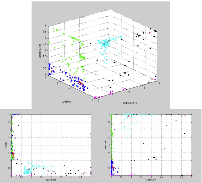
It was also tried to find the modes of all the fault clusters at the same time. The best result of this algorithm was obtained using 𝜎 = 0,35 ∗ standard deviation, as can be seen in the image 3.3:
3.2 - Information Theoretic Learning Mean Shift algorithm applications
Figure 3.3 - Database mode seeking output using ITLMS (𝝈 = 𝟎, 𝟑𝟓 ∗ 𝒎𝒆𝒂𝒏 𝒔𝒕𝒅 )
In the figure 3.3, in red are the outputs, in cyan are the high-energy discharge points, in blue the thermal fault with T<700ºC ones, the thermal fault with T>700ºC in green, in black the partial discharge representatives and in pink the low-energy discharge ones.
It can be seen that the algorithm couldn’t find a mode to the thermal fault with T>700ºC cluster and several ones are found to the thermal fault with T<700ºC, other problem happened in the low energy discharge cluster, where the mode found is highly influenced by the partial discharge points, being very inaccurate.
The different density of each cluster and the proximity between points of different clusters can justify these inaccuracies. Therefore, this result wasn’t used in any of the diagnosis methods.
Chapter 3.Densification of data sets
3.2.2. Densification trick using ITLMS
As mentioned before, one of the tasks done using the ITL Mean Shift algorithm was to create virtual data points to train neural networks, keeping the real data points to validate the results given by those networks. To do this, the same algorithm as the one used to find mode can be used, however with a slight difference: the results of all the iterations are kept. This means that the trajectory of any point until it reaches the mode, or any other cluster feature, is stored. This way, one point is used to create so many points as iterations. Due to the mean shift capacity of capturing the intrinsic properties of a data cluster, the virtual data points will be consistent with the real ones.
To create virtual data, a combination of the mean shift algorithm and the steepest descent one was used. While the mean shift algorithm was used to detect the path to the modes, the steepest descent algorithm was used in order to do the first iteration of the global algorithm. In this first iteration, the direction of the movement was the inverse direction of the attraction. This way, it is guaranteed that the real data does not form the frontier of the cluster. The iteration step that was used in the steepest descent algorithm was equal to -10. This was a value big enough to guarantee that the new point wasn’t too close to the original one, and small enough in order to keep the new point not too far from the original one. Once again, to adjust this parameter several tries were done.
All of the faults and healthy states were submitted to this algorithm in order to train the neural networks.
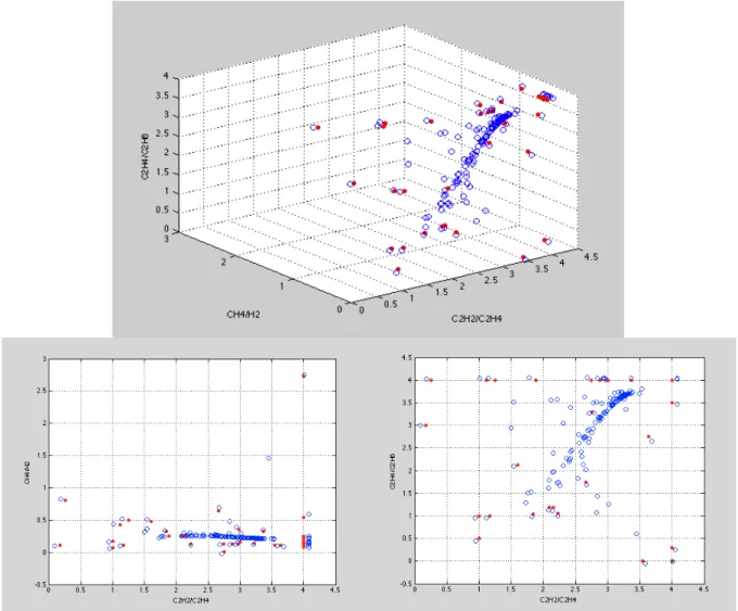
The result of this algorithm applied to the low-energy discharge, with the same parameters as the single mode-seeking algorithm (𝜆 = 1, 𝜎 = 𝑚𝑒𝑎𝑛 (𝑠𝑡𝑑)), can be seen in the figure 3.4. Once again, the red dots are the original data and the blue circles the virtual data.
3.2 - Information Theoretic Learning Mean Shift algorithm applications
Figure 3.4- Low-energy discharge ITLMS consecutive application (𝝀 = 𝟏, 𝝈 = 𝒎𝒆𝒂𝒏 (𝒔𝒕𝒅))
Doing a simple analysis to the figure 3.4, the first iteration can be clearly seen. These points are the new frontier of the cluster and guarantee that the real points are always inside, and never on the cluster limits. The points’ trajectory until the mode can be also observed. This new data set is the one used to train the networks.
Once again, this procedure was done to all the seven of transformers’ health states.
In order to compare the neural networks behaviour when trained with 𝜆 = 2 it was also done the densification trick with this value. When one uses 𝜆 = 2 the algorithm converges to the principal curve of the pdf. Principal curves give information about the cluster formed by the data and can be defined as non-parametric, smooth and one-dimensional curves that pass through the middle of a d-dimensional probability distribution or data set. [42, 54].
Since the algorithm is searching for different properties of the cluster, it returns different points, which can result in different neural network connection weights after training.
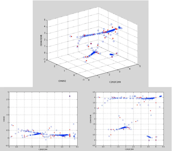
In figure 3.5, the output of the algorithm applied to the low energy discharge with 𝜆 = 2, 𝜎 = 𝑚𝑒𝑎𝑛 (𝑠𝑡𝑑) and the iteration step equal to -10, is shown.
Chapter 3.Densification of data sets
Figure 3.5 - Low-energy discharge fault ITMLS consecutive application (𝝀 = 𝟐, 𝝈 = 𝒎𝒆𝒂𝒏 (𝒔𝒕𝒅))
If one compares this figure with the one with 𝜆 = 1, it is easy to notice that both figures are very different. This is the result of seeking different properties of the pdf.
The output of this algorithm was used to train neural networks and the results are analysed in the proper chapter. Therefore, this procedure was done to all the faults/healthy states.
The use of virtual data points in the neural network training allows the use of all the real data in the validation stage. Thus, the results given by the validation process are more accurate, allowing one to have a better idea how the algorithm will behave when a new, completely unrelated data point is diagnosed.
In table 3.2 is the full description of the database obtained using 𝜆 = 1 and 𝜎 = 𝑚𝑒𝑎𝑛 𝑠𝑡𝑑 . The different values of virtual data can be justified with the number of the original real data and the number of iterations needed by the mean shift algorithm to converge to a single mode. Besides, for different ITLMS values the database can differ because of the number of iterations needed to the algorithm convergence.
3.2 - Information Theoretic Learning Mean Shift algorithm applications
Table 3.2 - Database complete description (using 𝝀 = 𝟏 and 𝝈 = 𝒎𝒆𝒂𝒏 𝒔𝒕𝒅 )
Case Fault/State Real Data Virtual Data
PD Partial Discharge 30 330
DH High Energy Discharge 103 618
DL Low energy Discharge 37 444
T1 Thermal Fault (T<700ºC) 77 1078
T2 Thermal Fault (T>700ºC) 71 639
OK Healthy State without OLTC 20 140
OK with OLTC Healthy State with OLTC 10 90
Chapter 3.Densification of data sets
3.2.1. Other ITLMS applications
As mentioned before, when one uses 𝜆 > 1 in the ITLMS algorithm, it seeks the cluster finer structures and these structures are more complex and have more information as 𝜆 increases. This way, and in order to study how the ITLMS and the diagnosis methods behave with this kind of data, several 𝜆 values were tested and it was concluded that the value where the best result were obtained was 𝜆 = 7. When the ITLMS algorithm is applied to the real data using 𝜆 = 7, the repulsion forced between the points is big enough to allowing the seeking of more structures intrinsic to the clusters, however this value isn’t too big to return only the real points (local modes) of the cluster.
The application of ITLMS with 𝜆 = 7 was done using several 𝜎 values and it was chosen the value which produced the most accurate results, being this value different between clusters. However, all the 𝜎 values chosen were between 0,5 ∗ 𝑚𝑒𝑎𝑛 𝑠𝑡𝑑 and 0,75 ∗ 𝑚𝑒𝑎𝑛 𝑠𝑡𝑑 .
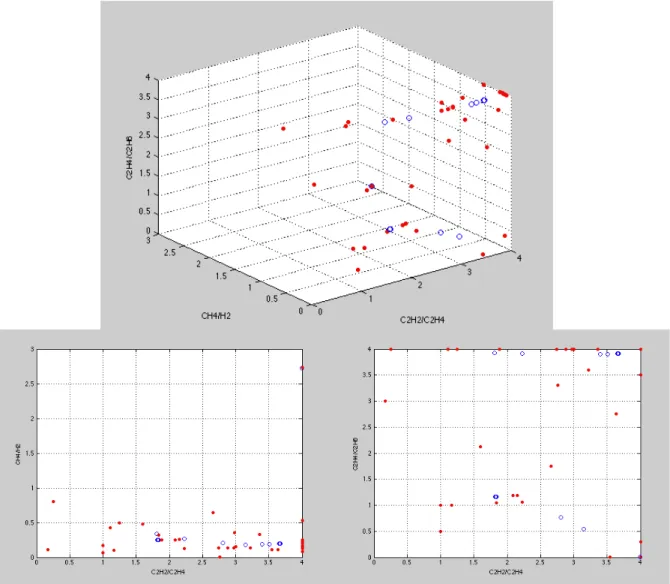
The results of the application of the ITLMS to the thermal fault (T>700ºC) cluster can be seen below, in image 3.6:
Figure 3.6– Thermal fault (T>700ºC) ITMLS finer structures seeking (𝝀 = 𝟕, 𝝈 = 𝟎, 𝟕𝟓 ∗ 𝒎𝒆𝒂𝒏 (𝒔𝒕𝒅))
Observing the figure it is possible to see some cluster structures which was the objective of this test.
3.2 - Information Theoretic Learning Mean Shift algorithm applications
With the same objective as before, seeking data that could improve the results given by the diagnosis methods, the ITLMS algorithm was applied to the real data with 𝜆 = 1 and 𝜆 = 2 using several 𝜎 values. The variation of 𝜎 values to smaller values allows the algorithm to seek for local modes, when 𝜆 = 1, or the principal curve in smaller spaces when 𝜆 = 2.
The output of the application of the ITLMS to the low-energy discharge data can be seen in the figure 3.7:
Figure 3.7 – Low-energy discharge fault ITLMS local modes seeking output (𝝀 = 𝟏, 𝝈 = 𝟎, 𝟓 ∗ 𝒎𝒆𝒂𝒏 (𝒔𝒕𝒅)) In figure 3.7 it is possible to see that most of the outputs (blue circles) of the algorithm are near the denser areas, as expected.
Chapter 4.
Incipient fault diagnosis systems
4.1. A diagnosis system using autoencoders
One of the first methods to diagnose power transformers that was studied as preparation for this thesis work was the one in [1].
In this method three dissolved gas concentration ratios are used as input, the same ones used in the IEC 60599 standard:
!!!! !!!!
!!! !!
!!!! !!!!
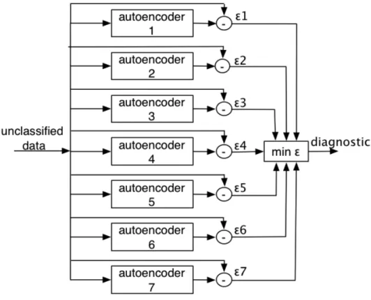
In spite of the fact that there are only six different states to the transformer condition, this method uses seven autoencoders, because it distinguishes between healthy transformers with and without on load tap changers (OLTC). Each of the networks is trained to recognize one fault and when a new input vector is shown to the system, all of the networks work in parallel, trying to replicate the input vector. However, just one of the autoencoders will produce an output very similar to the input one, i.e., it will resonate: it will show a very small error between the input and output, while in all the other autoencoders this error will be very high [52]. Thus, the method assumes that the unclassified data point belongs to the fault that this networks represents.
This method assumes that a data cluster with unique properties represents each one of the faults and that’s why there is one network per fault.
To build this diagnosing system, autoencoders with 3-15-3 architecture and neurons with sigmoid activation function were used. It has been shown that neurons with sigmoid activation functions induce better properties in feature reduction with autoencoders than the ones with linear activation functions [55]. When the middle layer of an autoencoder has neurons with linear activation functions it is equivalent to a Principal Component Analysis [56].
It must be said that these aren’t classical autoencoders because the neural networks’ hidden layers aren’t smaller than the input and output ones, so no data compressing is achieved. This isn’t one of the objectives, though
With systems architectures like this one, all networks are competing against the others when a new data point is presented. This is a great advantage because there are no unclassified samples after the diagnosis; however there can be wrong classifications. In the classic approach to this problem, where one single neural network is trained to recognize all the transformers’ health
Chapter 4. Incipient fault diagnosis systems
Other advantage of competitive architectures is that there is no need to set arbitrary thresholds. These parameters are used in order to decide if a point belongs or not to a certain faulty/healthy state. Having less parameters set in an arbitrary way means that there is no need to adjust those by trial and error and the methods adjustment to the data reality is easier and more accurate.
To train the neural networks, the neural network toolbox from MATALAB was used. The training algorithm used was the Levenberg-Marquardt one [57, 58] with the minimization of the mean square error as cost function. This cost function minimizes the variance in the probability density function of the error distribution, giving optimal results when the error distribution is Gaussian.
In order to have a better view of this system, a representative block diagram (figure 4.1) can be seen below:
Figure 4.4.1 - Autoencoders diagnosis system architecture
The results obtained with this system were satisfactory since 95,69% of correct diagnosis was achieved when the neural networks training was done using the ILTMS virtual data created using 𝜆 = 1 and 𝜎 adapted to retrieve a single mode. This means that 333 of 348 diagnoses were correct.
Also, using 𝜆 = 2 and 𝜎 = 𝑚𝑒𝑎𝑛(𝑠𝑡𝑑) in the mean shift algorithm in order to create virtual data and training autoencoders with these points retrieves 93,39% of correct diagnosis.
It must be said that training neural networks and especially autoassociative networks can be tricky because of the random initial weights MATLAB assigns. It took a long time to achieve this result and there is no guarantee that a better one can’t be accomplished; however a lot of tries were made.
4.1 - A diagnosis system using autoencoders
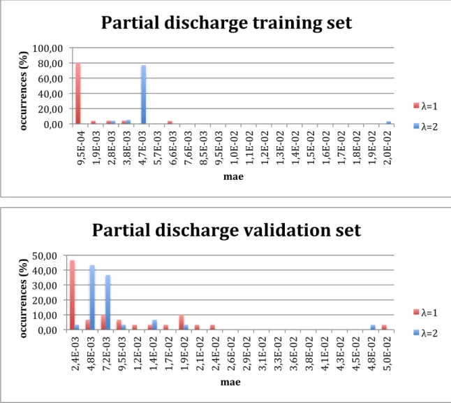
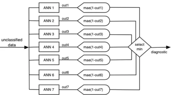
Training neural networks with data created with different 𝜆 values was done in order to compare which neural networks were more adapted to the data, i.e, which ones had a smaller input-output error. To do this study, the neural network that is supposed to recognize a given fault did the diagnosis for the corresponding fault data set (training and validation data) and the diagnosis error was stored. This diagnosis error was defined in this work as the mean absolute error between the input and output vectors. The interval between the maximum and the minimum error of each case was divided in 20 smaller intervals, allowing the building of the histograms of the figure 4.2:
Figure 4.2 - Partial discharge autoencoders diagnosys error comparison
In the partial discharge case, the results in the training set are fairly better when 𝜆 = 1, however in the validation set, the results obtained by using the data with 𝜆 = 2 slightly are better, with the first 3 columns summing 83,33% against 63,33% obtained by the neural networks trained with 𝜆 = 1 data. 0,00 10,00 20,00 30,00 40,00 50,00 2, 4E -‐0 3 4, 8E -‐0 3 7, 2E -‐0 3 9, 5E -‐0 3 1, 2E -‐0 2 1, 4E -‐0 2 1, 7E -‐0 2 1, 9E -‐0 2 2, 1E -‐0 2 2, 4E -‐0 2 2, 6E -‐0 2 2, 9E -‐0 2 3, 1E -‐0 2 3, 3E -‐0 2 3, 6E -‐0 2 3, 8E -‐0 2 4, 1E -‐0 2 4, 3E -‐0 2 4, 5E -‐0 2 4, 8E -‐0 2 5, 0E -‐0 2 oc cu rr en ce s (% ) mae
Partial discharge validation set
λ=1 λ=2 0,00 20,00 40,00 60,00 80,00 100,00 9, 5E -‐0 4 1, 9E -‐0 3 2, 8E -‐0 3 3, 8E -‐0 3 4, 7E -‐0 3 5, 7E -‐0 3 6, 6E -‐0 3 7, 6E -‐0 3 8, 5E -‐0 3 9, 5E -‐0 3 1, 0E -‐0 2 1, 1E -‐0 2 1, 2E -‐0 2 1, 3E -‐0 2 1, 4E -‐0 2 1, 5E -‐0 2 1, 6E -‐0 2 1, 7E -‐0 2 1, 8E -‐0 2 1, 9E -‐0 2 2, 0E -‐0 2 oc cu rr en ce s (% ) mae
Partial discharge training set
λ=1 λ=2
Chapter 4. Incipient fault diagnosis systems
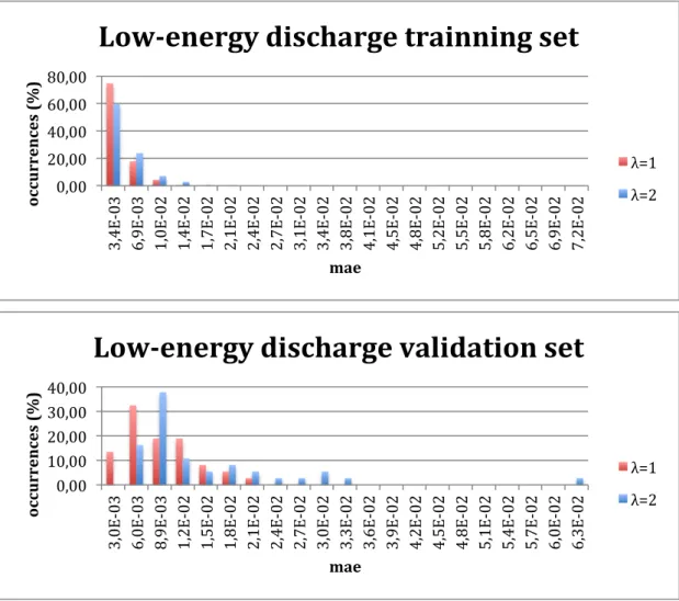
Figure 4.3 - Low-energy discharge autoencoders diagnosys error comparison
In what concerns the low-energy discharge data, presented in figure 4.3, the diagnosis of both sets are better when the neural networks are trained with the 𝜆 equal to one. This result is similar in the remaining faults/healthy states. The networks give better results when trained with virtual data created using 𝜆 = 1.
The results show that neural networks can have better results when trained with data created using the ITLMS with 𝜆 = 1 or 𝜆 = 2. This is related with the cluster pdf shape, i.e. a cluster with a pdf with a paraboloid shape doesn’t have a principal curve and will have better results with 𝜆 = 1. When a neural network is trained with virtual data created using different 𝜆 values, one is adapting the method to the shape and intrinsic properties of the cluster; therefore, the results obtained should be better. When the pdf of a given cluster doesn’t have a principal curve and 𝜆 = 2 is used in the ITLMS, the points will spread in the surroundings of the mode, however, because repulsion between the points is bigger, they do not converge to a single point/mode.
Due to this study results, an attempt to create a diagnosis method using neural networks trained with different 𝜆 values was made. The partial discharge autoencoder was trained with 𝜆 = 2 data and the other six faults/healthy states were trained with data created by the ITLMS algorithm using 𝜆 = 1. This way, 95,98% of correct diagnosis was achieved. This is a slight improvement of 0,3% in comparison with the method with all the neural networks trained using 𝜆 = 1 data.
0,00 20,00 40,00 60,00 80,00 3, 4E -‐0 3 6, 9E -‐0 3 1, 0E -‐0 2 1, 4E -‐0 2 1, 7E -‐0 2 2, 1E -‐0 2 2, 4E -‐0 2 2, 7E -‐0 2 3, 1E -‐0 2 3, 4E -‐0 2 3, 8E -‐0 2 4, 1E -‐0 2 4, 5E -‐0 2 4, 8E -‐0 2 5, 2E -‐0 2 5, 5E -‐0 2 5, 8E -‐0 2 6, 2E -‐0 2 6, 5E -‐0 2 6, 9E -‐0 2 7, 2E -‐0 2 oc cu rr en ce s (% ) mae
Low-‐energy discharge trainning set
λ=1 λ=2 0,00 10,00 20,00 30,00 40,00 3, 0E -‐0 3 6, 0E -‐0 3 8, 9E -‐0 3 1, 2E -‐0 2 1, 5E -‐0 2 1, 8E -‐0 2 2, 1E -‐0 2 2, 4E -‐0 2 2, 7E -‐0 2 3, 0E -‐0 2 3, 3E -‐0 2 3, 6E -‐0 2 3, 9E -‐0 2 4, 2E -‐0 2 4, 5E -‐0 2 4, 8E -‐0 2 5, 1E -‐0 2 5, 4E -‐0 2 5, 7E -‐0 2 6, 0E -‐0 2 6, 3E -‐0 2 oc cu rr en ce s (% ) mae
Low-‐energy discharge validation set
λ=1 λ=2
4.1 - A diagnosis system using autoencoders
The neural networks constituents of this diagnosis method were also trained with the ITLMS virtual data created using 𝜆 = 1 , 𝜆 = 2 and 𝜆 = 7 and 𝜎 and various 𝜎 values for the different clusters. The results for each one were 94,54%, 94,83% and 79,6%. The diagnosis result obtained with 𝜆 = 2 and various 𝜎 values, where the ITLMS returns the principal curve of smaller zones in the space, is better than the one obtained using 𝜆 = 2 and 𝜎 = 𝑚𝑒𝑎𝑛(𝑠𝑡𝑑).
The results obtained with this method are summarized in the following table: Table 4.1 – Autoencoder method results summary
𝝀 𝝈 Results (%) 1 mean(std) 95,69 2 mean(std) 93,39 1 and 2 mean(std) 95,98 1 various 94,54 2 various 94,83 7 various 79,6
In table 4.1, where 𝜎 appears as various is because the value was adapted to each cluster in order to the ITLMS return the characteristic sought.
![Figure 2.1 - IEC60599 graphical representation of gas ratios [2]](https://thumb-eu.123doks.com/thumbv2/123dok_br/15733898.1071783/19.892.256.638.165.505/figure-iec-graphical-representation-gas-ratios.webp)