Abstract
In the present paper, the aerothermoelastic behavior of Functiona-lly Graded (FG) plates under supersonic airflow is investigated using Generalized Differential Quadrature Method (GDQM). The structural model is considered based on the classical plate theory and the von Karman strain-displacement relations are utilized to involve the nonlinear behavior of the plate. To consider the super-sonic aerodynamic loads on the plate, the first order piston theory is applied. The material properties of the FG panel are assumed to be temperature independent and alter in the thickness direction according to a power law distribution. The temperature distribu-tion on the surface of the plate is assumed to be constant and in the thickness direction is obtained by one-dimensional steady conductive heat transfer equation. The discretized governing equa-tions via GDQM are solved by the fourth order Runge-Kutta method. Comparison of the obtained results with those available in literature confirms the accuracy and ability of the GDQM to perform the aerothermoelastic analysis of FG plates. Also, the effect of some important parameters such as Mach number, in-plane thermal load, plate aspect ratio and volume fraction index on the plate aerothermoelastic behavior is examined.
Keywords
Differential Quadrature Method, Aerothermoelastic, Functionally Graded Material, Stability boundary.
Aerothermoelastic Analysis of Functionally Graded Plates
Using Generalized Differential Quadrature Method
1 INTRODUCTION
The lifting surfaces and panels of space re-entry vehicles and high-speed aircrafts are exposed to combined effects of aerodynamic, thermodynamic, inertial, and elastic forces. One of the key factors in the design of their outer skins is the aerothermoelastic considerations. In this regard many re-searches have been performed.
H. Shahverdi a V. Khalafi b S. Noori c
a, b, c Department of Aerospace
Engineer-ing and Center of Excellence in Compu-tational Aerospace Engineering, Amirka-bir University of Technology, Tehran, Iran
Author email:
a Corresponding author,
b [email protected] c [email protected]
http://dx.doi.org/10.1590/1679-78252072
The first studies on the flutter behavior of a panel can be traced back to the works of Houbolt (1958), Bolotin (1963) and Dowell (1966, 1975). Schaeffer and Heard (1965) studied aeroelastic re-sponse of a flat panel exposed to a nonlinear temperature distribution with simply support bounda-ry conditions. Xue and Mei (1993a) investigated the nonlinear flutter response of isotropic panels under thermal effects using FEM. To account for structural nonlinearity, von Karman's large de-tion plate theory was considered. They studied the effects of nonuniform temperature distribude-tion, panel aspect ratio, and boundary conditions on the flutter behaviors of rectangular and triangular panels. Also, Xue and Mei (1993b) considered the fatigue life of isotropic panels in frequency do-main using FEM and investigated the effect of dynamic pressure and temperature onthe fatigue life of a panel.
In the modern structures, a new material with desired mechanical and strength properties is generated by combining of different material layers. Thus, Isotropic materials have been replaced by composite materials. In the recent decades, Functionally Graded Materials (FGMs) have attracted considerable attention as materials for various advanced purposes. Functionally graded materials are a new type of inhomogeneous materials and advanced composites. A functionally graded mate-rial is usually a combination of two matemate-rials or phases that have gradual transition of properties from one side of sample to another side. This gradual transition allows the thermo-mechanically interface problems in a composite structure such as sharp local stress concentration, delamination and weak thermal resistance, can be impressively decreased (Miyamoto et al., 1999). Across the consecutive development of FGMs, there have been many research works as follows. Praveen and Reddy (1998) investigated the static and dynamic response of functionally graded plates using a plate finite element that accounted for the effects of the transverse shear strains, rotary inertia and the moderately large rotations in the von Karman sense. They showed that the response of the plates with material properties between those of the ceramic and metal is not intermediate to the responses of the ceramic and metal plates. Javaheri and Eslami (2002) derived stability equations of a rectangular functionally graded plate using with the classical plate theory. Sohn and Kim (2008) analyzed structural stability of functionally graded panels under simultaneous thermal and aerody-namic loads. In this work, thermal post-buckling behaviors and stability boundaries for clamped and simply support FG panels with uniform temperature gradients were studied. Sohn and Kim (2009) studied the aerothermoelastic instability of FGM panels in supersonic flow and showed the effects of the volume fraction distributions, temperature changes, aerodynamic pressures and the boundary conditions on the panel flutter. Navazi and Haddadpour (2011) analyzed the nonlinear flutter behavior and stability boundaries of isotropic and FGM plates in supersonic airflow, and showed that under real flight conditions and using coupled model, the aerodynamic heating is very severe and the type of instability is divergence. Janghorban and Zare (2011) examined the vibration analysis of a functionally graded plate with cutouts and skew boundary. In this work, the role of different parameters such as cutout size, type of loading and different boundary conditions on the vibration of the plate was reported. Taj and Chakrabarti (2013) investigated a finite element formu-lation based on Reddy’s higher order theory to investigate the dynamic response of a FG skew shell.
main idea behind the DQM is that the derivative of a function with respect to a space variable at a given point is approximated as a weighted linear sum of the function values at all discrete points along the domain of that variable.
The DQM has been applied to solve various structural elements such as beams, plates and shells. Bert et al. (1988) applied the DQM to investigate static and dynamic response of structures for the first time, and afterwards it was improved by Bert and Malik (1996). Also, Bert et al. (1989) used DQM for composite plates for the first time and analyzed nonlinear bending of orthotropic rectangular plates. Then, Shu and Richards (1992) presented the GDQM to simplify the computa-tion of the weighting coefficients. Shu and Wang (1999) applied GDQM for vibration analysis of a rectangular plate with combined and non-uniform boundary conditions. Fazelzadeh et al. (2007) investigated the vibration of a rotating thin walled-blade made of functionally graded materials operating under high temperature supersonic gas flow with DQM. Talebitooti et al. (2013) present-ed the effects of boundary conditions and axial loading on the frequency characteristics of rotating laminated conical shells with orthogonal stiffeners using GDQM.
This paper extends the application of the DQM to aerothermoelastic analysis of a flat plate in supersonic flow. In this regard the governing differential aeroelastic equations of a FG plate as first discretized using GDQM and then aerothermoelastic response of the plate is studied by the fourth order Runge-Kutta method. To demonstrate the accuracy and fidelity of the GDQM, the dynamic stability boundaries of the plate are validated with available results presented by other researchers. Also, the effects of some important parameters such as Mach number, in-plane thermal load, plate aspect ratio and volume fraction index on the plate aerothermoelastic behavior are investigated.
2 FORMULATION
2.1 Structural Model
A plate with length a, width b, and thickness h made up of a mixture of ceramic and metal is con-sidered. The airflow is assumed in the x-direction. Volume fraction of the functionally graded mate-rial varies continuously through the plate thickness according to a simple power law (Javaheri and Eslami, 2002). Hence:
/ 2
n mz h
V
h
(1)
V
m
V
c1
(2)where z is the coordinate in the thickness direction with origin at the plate mid-surface and n is the volume fraction index. Thus, the material properties of the functionally graded plate can be ex-pressed as
eff m m c c
/ 2
neff c m m
z
h
P
P
P
P
h
(4)where subscripts c and m refer to ceramic and metal, respectively, and Peff is the effective material properties of the plate corresponding to the modulus of elasticity
E , Poisson’s ratio
, density
and thermal coefficient expansion
.Based on the Classical Plate Theory (CPT), the displacement field of the plate is:
0 0
0 0
0
( , , )
( , , , )
( , , )
( , , )
( , , , )
( , , )
( , , , )
( , , )
w x y t
u x y z t
u x y t
z
x
w x y t
v x y z t
v x y t
z
y
w x y z t
w x y t
(5)
where u0 and v0 are the in-plane displacement components, and w0 is the out-of-plane displacement component measured from the plate’s mid-plane.
According to the von Karman nonlinear strain-displacement relations, the nonlinear strains are defined as:
0
z k
(6)where
0andk
are the mid-plane membrane and bending strain vectors, respectively, which can be defined as follows:
0 2
0, 0,
0 0 2
0, 0,
0
0, 0, 0, 0,
1
2
2
xx x x
yy y y
xy y x x y
u
w
v
w
u
v
w w
(7)
2
xx xx
yy yy
xy xy
k
w
k
k
w
k
w
(8)
The thermoelastic constitutive equations of the FG panels are:
11 12
12 22
66
0
,
( )
0
,
( )
0
0
xx xx
yy xx
xy xy
Q
Q
z T
T z
Q
Q
z T
T z
Q
(9)
0
( )
( )
T z
T z
T
where T0, T(z) and
( , )
z T
are reference temperature, temperature distribution in the plate thick-ness direction and thermal expansion coefficient, respectively. Qij are the elements of material con-stant matrix and defined by
11 22 2
12 2
66
( )
1
( )
( ) ( )
1
( )
( )
2 1
( )
E z
Q
Q
z
z E z
Q
z
E z
Q
z
(11)
where E(z) is the elastic modulus of a FG panel.
In-plane force resultant and out-of-plate moment resultant are obtained as follows:
0 T
T
k
N
A
B
N
M
B
D
M
(12)Here, NT and MT are the thermal in-plane force and moment resultant vectors. Thus
2 2( )
,
(1, )
( )
( )
0
hT T
h
z
z
z
T z dz
N
M
Q
(13)while A, B and D are extension, bending–extension coupling, and bending stiffness and are given as follows:
11 12 11 12 11 12
12 22 12 22 12 22
66 66 66
0 0 0
0 , 0 , 0
0 0 0 0 0 0
A A B B D D
A A B B D D
A B D
A B D (14)
2 2
2
(
,
,
)
(1, ,
)
h h
ij ij ij ij
A B D
Q
z z dz
(15)2.2 Aerodynamic Model
According to the first order piston theory (Dowell, 1975), the aerodynamic pressure, may be ex-pressed as
2
2 2
2 1 2
( )
1 1
q M w w
p
U M t x
M
where q, M and
U
represent the dynamic pressure, Mach number, and the free stream velocity, respectively. The linear piston theory is valid for2
M
5
(Mei et al., 1999).2.3 Temperature Distribution
The temperature distribution on the surface of the plate is assumed to be constant while in the thickness direction it is considered to be variable and may be obtained by solving the one-dimensional Fourier equation of the heat conduction, which is
2
( )
0 ,
2
cm
h
T
T
at z
d
dT
K z
h
dz
dz
T
T
at z
(17)
Tm and Tc are the temperature of the lower and upper surfaces of the panel, and temperature dis-tribution in the plate thickness direction is obtained by means of polynomial series (Javaheri and Eslami, 2002) and given as follows:
( )
m(
c m) ( )
T z
T
T
T
z
(18)where
( 1) 2 (2 1)
2
(3 1) (4 1) (5 1)
3 4 5
3 4 5
(
)
(
)
1
1
1
1
( )
2
(
1)
2
(2
1)
2
(
)
1
(
)
1
(
)
1
(3
1)
2
(4
1)
2
(5
1)
2
n n
c m c m
m m
n n n
c m c m c m
m m m
K
K
K
K
z
z
z
z
C h
K
n
h
K
n
h
K
K
z
K
K
z
K
K
z
K
n
h
K
n
h
K
n
h
(19)
2 3 4 5
2 3 4 5
(
)
(
)
(
)
(
)
(
)
1
(
1)
(2
1)
(3
1)
(4
1)
(5
1)
c m c m c m c m c m
m m m m m
K
K
K
K
K
K
K
K
K
K
C
K n
K
n
K
n
K
n
K
n
(20)2.4 Equations of Motion
By means of the extended Hamilton’s principle, the nonlinear governing equations of motion can be obtained. In the absence of surface shearing forces, body moments and inertial forces in the x and y directions, the aeroelastic equations of a FG plate are (Bert et al., 1989)
, ,
, ,
2 2 2 ..
, , , 2 2 0
0
0
2
2
xx x xy y
xy x yy y
xx xx xy xy yy yy xx xy yy
N
N
N
N
w
w
w
M
M
M
N
N
N
p
I w
x
x y
y
(21)
2
0
2
( )
h h
I
z dz
(22)By substituting the Eqs. (9) and (12) into Eq. 21, the equations of motion are obtained as fol-lows:
11 12 11 12 66 66
0
yy yy xy xy
xx
k
xxk
k
A
A
B
B
A
B
x
x
x
x
y
y
(23)12 22 12 22 66 66
0
yy yy xy xy
xx
k
xxk
k
A
A
B
B
A
B
y
y
y
y
x
x
(24)2 2
2 2 2
11 2 12 2 11 2 12 2 12 2
2 2 2 2 2
22 2 12 2 22 2 66 66
2 2 2 ..
0
2 2
2
2
2
yy yy
xx xx xx
yy xx yy xy xy
xx xy yy
k
k
B
B
D
D
B
x
x
x
x
y
k
k
k
B
D
D
B
D
y
y
y
x y
x y
w
w
w
N
N
N
p
I w
x
x y
y
(25)By differentiating from Eq. (23) and Eq. (24) with respect to the variable of x and y, respective-ly, and summing the resultant equations, we will have
2 2 2 2
2 2
11 2 12 2 11 2 12 2 66 66
2 2 2 2
2 2
12 2 22 2 12 2 22 2 66 66
0
yy yy xy xy
xx xx
yy yy xy xy
xx xx
k
k
k
A
A
B
B
A
B
x
x
x
x
x y
x y
k
k
k
A
A
B
B
A
B
y
y
y
y
x y
x y
(26)By multiplying
B
11 to Eq. (25) andA
11to Eq. (26) and substituting Eq. (25) into Eq. (26) and after some mathematical manipulations, the following equation is obtained.2
2 2
2 2 2
11 11 11 11 11 11 11 11 11
2 2 2
11 11 11
2 2
2 2 2 2
11 11 11 11 11 11
2 2 11 11 2 .. 0 2
(
)
(
)
(
)
(
)
1
(
)
2
2
2
yy xx xx yy xy xx xy yyk
k
k
D A
B
D A
B
D A
B
A
x
A
x
A
y
k
k
D A
B
D A
B
w
w
N
N
A
y
A
x y
x
x y
w
N
p
I w
y
(27)The above equation can be written as
4 4 4 2 2 2 ..
0
4
2
2 2 4 22
20
eq xx xy yy
w
w
w
w
w
w
D
N
N
N
p
I w
x
x y
y
x
x y
y
where
2
11 11 11
11
eq
D A
B
D
A
(29)In this paper, the plate is considered to be simply supported along all edges and therefore the in-plane displacement components u, v, u, v
x y y x
are equal to zero and based on this assumption
the in-plane force resultants can be modified as follows (Dowell 1975, Miller et al., 2011):
2 2
2 2
11 12 11 2 12 2
0 0
2 2
2 2
12 22 12 2 22 2
0 0 2 66 66 0 0
1
1
(
)
(
)
2
2
1
1
(
)
(
)
2
2
2
b a T
xx xx b a T yy yy b a xy
w
w
w
w
N
A
A
B
B
dxdy
N
x
y
x
y
w
w
w
w
N
A
A
B
B
dxdy
N
x
y
x
y
w w
w
N
A
B
dxdy
x
y
x y
(30)By substituting Eqs. (16) and (31) into Eq. (28), the aerothermoelastic equation is obtained.
4 4 4
4 2 2 4
2 2 2
2 2
11 12 11 2 12 2 2
0 0 2 2 66 66 0 0 2 2 2
12 22 12 2 2
2
1
1
(
)
(
)
2
2
2
2
1
1
(
)
(
)
2
2
eq b a b aw
w
w
D
x
x y
y
w
w
w
w
w
A
A
B
B
dxdy
x
y
x
y
x
w w
w
w
A
B
dxdy
x
y
x y
x y
w
w
w
A
A
B
B
x
y
x
2 22 2 2
0 0
2 2 2 ..
0
2 2 2
2
2
0
1
b a T T xx yyw
w
dxdy
y
y
q
w
w
w
M
w
N
N
U
I w
x
y
U
x
M
t
(31)In a supersonic regime, the coefficient of the aerodynamic damping in Eq. (31) can be approxi-mately expressed as (Liaw and Yang, 1993)
2 2 2 2
2
1
1
M
M
M
M
(32)3
1 2
4
2 2
2
m
m
m m
T T
yy xx
x y
m m
w
x
W
h
a
q a
y
b
D
D
a
t
h
ha
N
b
N
a
R
R
D
D
(33)
By introducing the above parameters into Eq. (31), the non-dimensional form of aeroelastic equations can be obtained.
2 4
2 4 4 4
0
2 4 2 2 4
2 3 2 2 3 2 2
1 1 2 2
11 12 11 2 12 2 2
0 0
3 2 3 2
66 66
2
(
)
(
)
2
2
2
2
eq
m m
m m m m
m m
D
I
W
W
a
W
a
W
h
D
b
b
abh
W
a h
W
abh
W
a h
W
W
A
A
B
B
d d
D
bD
D
bD
a h
W W
a h
W
A
B
bD
bD
2 1 1
0 0
3 2 2 3 2 2 2
1 1 2 2
12 22 12 2 22 2 2
0 0
2
2 2
2 2
(
)
(
)
2
2
0
m m m m
x y
W
d d
a h
W
abh
W
a h
W
abh
W
W
A
A
B
B
d d
bD
D
bD
D
W
a
W
W
W
R
R
b
M
(34)
3 DISCRETIZED FORM OF THE GOVERNING EQUATION
In this section, the governing aeroelastic equation is discretized by using the GDQM. This method implies that the rth-order derivative of a function W, at a point s = si , with N discrete points can be estimated by
( )
1
i
r N
r s
s s ij j
r
j
W
A W
s
(35)The coefficient
A
ij( )r srepresents the weighting coefficeints. The method for constructing theseco-efficients can be found in Chang Shu (2000).
( )
( ) ( )
1 1
r s N M
r x s y
ik jl kl
r s k l
W
A
A
W
x y
(36)0 0
1 1
( , )
N M
a b
k l kl k l
W x y dxdy
c c W
(37)where
c c
l,
kare the weighting coefficients of the one-dimensional integral in the x and y directions respectively, and given by (Chang Shu, 2000)( ) ( )
0
( )
a
I x I x
k jk ik k
c
H
H
r x dx
(38)( ) ( )
0
( )
b
I y I y
l jl il l
c
H
H
r y dy
(39)where
( ) (1) 1 ( ) (1) 1
(
)
,
(
)
I x x I y y
H
A
H
A
(40)In the above equations
r x
k( )
andr y
l( )
are the Lagrange interpolated polynomials. By using the DQM, the discretized form of the governing equations (Eq. 34) can be written as:2 4
(4) ( 2) ( 2) ( 4)
0
1 1 1 2 1 2 2 2
1 1 1 1 2 1 2 1
2
(1) (1) ( 2) 11
, , , 1 1 3 2 (1 12 2 2 2
N N M M
eq
ik k j ik jk k k jk ik
k k k k
m m
N M
x x x
k p kn pm il kn pm lj k l m n p
m
k p kq m
D
I a a
W W Ax W Ay Ay W Ay W
h M D b b
abh
A c c A A A W W W
D a h
A c c A
bD
) (1) (2)
, 1 , , 1
3
(2) (2) (2) ( 2)
11 12
, , 1 1 , 1 , 1
3 2
(1) (1) (1) (1)
66 1 2
, 1, 1 , 2, 1 2
N M
y y x
ps il kq ps lj k l p q s
N M N M
x x y x
k p kn il pn lj k p pq il kq lj
k l n p k l p q
m m
M
x y x y
k p kn pq ik jk k k n p k q
m
A A W W W
abh a h
B c c A A W W B c c A A W W
D bD
a h
A c c A A A A
bD
1 23
(1) (1) (1) (1)
66 1 2 1 2
, 1, 1 , 2, 1 3 2
(1) (1) (2) 12
1 , , , 1 2
(1) (1) (2) 22
, , 1 , 1 4
2
2
N
kn pq k k
N M
x y x y
k p kn pq ik jk nq k k k k n p k q
m
N M
x x y
k p ks pt jq ks pt iq k p q t s
m
N M
y y y
k p pm kn jq k m n p q
m
W W W
a h
B c c A A A A W W
bD a h
A c c A A A W W W
bD abh
A c c A A A
D
3( 2) (2) (2) (2)
12 22
1 , , 1 , 1 , 1
pm kn iq
N M N M
x y y y
k p pt jq kt iq k p kn jq pn iq
k p q t k n p q
m m
W W W
a h abh
B c c A A W W B c c A A W W
bD D
4
(2) (2) (1)
1 1 2 2 1
1 1 2 1 1 1
0
, , , , , 1 1, 2,...,
, , , , , 2 1, 2,...,
N M N
x y x
x ik k j y jk ik ik k j
k k k
a
R
A
W
R
A
W
A W
b
for i k k m n k
N
j p q s t k
M
Also, the assumed boundary conditions may be defined as follows:
2 2 2 2 2 2 2 2
(0, , )
(0, , )
0,
0
( , , )
( , , )
0,
0
( , 0, )
( , 0, )
0,
0
( , , )
( , , )
0,
0
w
y t
w
y t
x
w a y t
w a y t
x
w x
t
w x
t
y
w x b t
w x b t
y
(42)The discretized form of these boundary conditions will be:
( 2)
1, 1, ,
1
( 2)
, , ,
1
( 2)
,1 1, ,
1
( 2)
, , ,
1
0 ,
0
0
0 ,
0
1
0 ,
0
0
0 ,
0
0
N x
j k k j
k N
x
N j N k k j
k M
x
i k i k
k M
x
i M M k i k
k
W
A
W
at
W
A
W
at
W
A
W
at
W
A
W
at
(43)Thus, the boundary conditions can be written as:
1 ( 2) 1, , 2 1 ( 2) , , 2 1 ( 2) 1, , 2 1 ( 2) , , 2
0
0
0
0
N x k k j kN x N k k j k
M x k i k k
By incorporating the boundary conditions into Eq. (41) and doing some manipulations, the final aerothermoelastic equation of a FG plate can be drawn as:
2 4
2 2 2 2
0
1 2 1 2 3
3 1 3 2 3 3
2 2 2 3 2 2 2
11 4 12 5
, , , 3 3 , 3 , , 3
2
2
2
N N M M
eq
kj k k ik
k k k k
m m
N M N M
kn pm lj kp mn lj
k l m n p k l m n p
m m
D
I
a
a
W
W
C W
C W
C W
h
M
D
b
b
abh
a h
A
C W W W
A
C W W W
D
bD
3
2 2 2 2
11 6 12 7
, , 3 3 , 3 , 3
3 2 2 2 3 2 2
66 8 1 2 66 9 1 2
, 1, 3 , 2, 3 , 1, 3 , 2, 3
3 2 2 2
12 10
3 , , , 3
2
4
2
N M N M
pn lj kq lj
k l n p k l p q
m m
N M N M
kn pq k k nq k k
k k n p k q k k n p k q
m m
N M
k p q t s m
abh
a h
B
C W W
B
C W W
D
bD
a h
a h
A
C W W W
B
C W W
bD
bD
a h
A
C
bD
2 2 222 11
, , 3 , 3
3 2 2 2 2 2
12 12 22 13 14
3 , , 3 , 3 , 3 3
4 2 2
15 16
3 3
2
0
, , , , , 1
3
N M
ks pt iq pm kn iq
k m n p q m
N M N M N
kt iq pn iq x kj
k p q t k n p q k
m m
M N
y ik kj
k k
abh
W W W
A
C W W W
D
a h
abh
B
C W W
B
C W W
R
C W
bD
D
a
R
C W
C W
b
for i k k m n k
, 4,...,
2
, , , , , 2
3, 4,...,
2
N
j p q s t k
M
(45)
where C1 to C16 are defined in Appendix A
4 RESULTS AND DISCUSSION
In this section, the critical dynamic pressures for FG plates are calculated to investigate the validity of the GDQM for determining flutter boundaries. In this regard, a simply-supported functionally graded flat plate made of a combination of metal (SUS304) and ceramic (Si3N3) is considered as a
test case. The material properties are listed in Table 1 (Navazi and Haddadpour, 2011).
Material
Young's modulus
(GPa)
Poisson's ratio
Mass den-sity (Kg/m3)
CTE (1/K)
Thermal conductivity
(W/mK)
SUS304 207.8 0.3 7800 1.53E-05 1.214E+01
Si3N3 322.3 0.3 3200 7.47E-06 1.011E+01
Table 1: Material properties at reference temperature (T= 300 K)
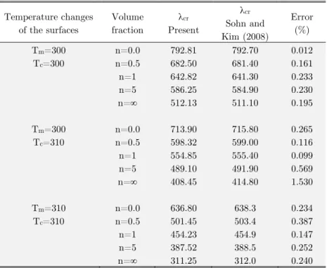
Table 2 shows the obtained critical non-dimensional dynamic pressures (λcr) of a FG square plate with a/b=1(aspect ratio), a/h=100 (length/ thickness ratio) along with those reported by Sohn and Kim (2008) under different volume fractions and temperatures. It is clear that the ob-tained results are in good agreement with Sohn and Kim (2008).
Temperature changes of the surfaces
Volume fraction
λcr
Present
λcr
Sohn and Kim (2008)
Error (%)
Tm=300 n=0.0 792.81 792.70 0.012
Tc=300 n=0.5 682.50 681.40 0.161
n=1 642.82 641.30 0.233
n=5 586.25 584.90 0.230
n= 512.13 511.10 0.195
Tm=300 n=0.0 713.90 715.80 0.265
Tc=310 n=0.5 598.32 599.00 0.116
n=1 554.85 555.40 0.099
n=5 489.10 491.90 0.569
n= 408.45 414.80 1.530
Tm=310 n=0.0 636.80 638.3 0.234
Tc=310 n=0.5 501.45 503.4 0.387
n=1 454.23 454.9 0.147
n=5 387.52 388.5 0.252
n= 311.25 312.0 0.240
Table 2: Critical non-dimensional dynamic pressure
Next, to validate the post flutter characteristics of the present computational model, the limit cy-cle amplitudes of an isotropic square panel for various dynamic pressures, at a specified location (
0 .7 5and
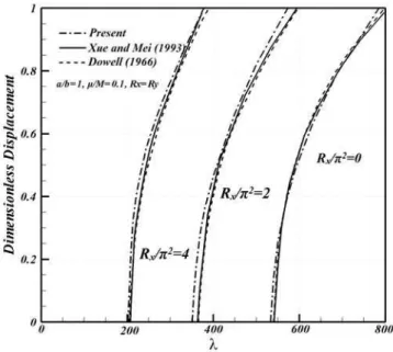
0 .5 ) on the panel are computed and depicted in Fig. 1. As is evident, theFigure 1: LCO amplitudes of the isotropic square panel
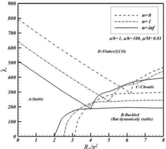
Finally, the aerothermoelastic stability boundaries of the panel according to in-plane thermal load are depicted in Fig. 2. As shown in this figure, the developed tool can capture different dynam-ic behaviors of the plate, including stable, limit cycle oscillation (LCO), Buckled and chaotdynam-ic, as well as Xue and Mei (1993).
Figure 2: Stability boundaries of the isotropic square panel
the other hand, any increase in volume fraction index leads to reduction in the critical dynamic pressure. However, this reduction is impressive until the value of volume fraction becomes about unity.
The effects of aspect ratio (a/b) on the critical dynamic pressure are presented in Fig. 4. It can be seen that the critical dynamic pressure increases with the plate aspect ratio. Moreover, the variation of critical dynamic pressure with respect to µ/M is more dominant for plates with higher aspect ratio.
n
C
ri
ti
c
al
D
y
n
a
m
ic
P
re
ssu
re
0 2 4 6 8 10
550 600 650 700 750 800 850
µ/M= 0.01 µ/M= 0.05 µ/M= 0.1
Figure 3: Effect of µ/M on the critical dynamic pressure of the FG panel (a/h=100)
n
C
riti
c
a
l
D
y
n
a
m
ic
P
re
ss
u
re
0 2 4 6 8 10
200 400 600 800 1000 1200 1400
µ/M= 0.01 µ/M= 0.1
a/b= 1.5
a/b= 1
a/b= 0.5
The limit cycle amplitude of the FG plate at the aforementioned pointversus the critical dy-namic pressure for various volume fraction indexes and different values of Tc is shown in Figure 5. It should be noted that the value of Tc is considerd to vary from 300 K (the gary lines) to 320 K (the black lines) and Tm is taken to be 300 K. It is found that by increasing the surface tempera-ture of the FG plate, the critical dynamic pressure is decreased.
D
im
e
n
sio
n
le
ss
D
is
p
la
c
em
e
n
t
0 200 400 600 800 1000 0
0.2 0.4 0.6 0.8
n= inf n= 3 n= 1 n= 0.3 n= 0 n= inf n= 3 n= 1 n= 0.3 n= 0
Figure 5: Deflection LCO dimensionless amplitude of the FG panel.
The aerothermoelastic stability margins versus in-plane thermal load for various volume frac-tion indexes are shown in Fig. 6. It can be seen that as the volume fracfrac-tion index decreases the critical thermal buckling load, the critical dynamic pressure and the in-plane thermal load, where the chaotic motion begins, all increase. As a result, the bifurcation point shifts to the top right.
As shown in Fig. 6, the plate remains stable in zone A. The typical time history of this zone is shown in Fig. 7.
Dimensionless Time
D
im
en
si
o
n
les
s
D
is
p
la
cem
en
t
0 2 4 6 8 10
-0.4 -0.2 0 0.2 0.4
Figure 7: Non-dimensional deflection of the panel (λ=350, n=1, Rx=Ry=3π2)
In zone B, the panel is dynamically stable, but statically unstable and buckled. The dimension-less deflection time histories in zone B for two specific conditions are shown in Figs. 8 and 9. They reveal that the steady response of the panel increases with increasing of n. They also show that the amplitude of the panel motion decreases with increasing of dynamic pressure.
Dimensionless Time
D
im
e
ns
io
nl
e
ss
D
is
p
la
c
e
m
e
n
t
0 2 4 6 8 10
0 0.2 0.4 0.6 0.8 1
Dimensionless Time
D
im
e
ns
io
nl
e
ss
D
is
p
la
c
e
m
e
nt
0 2 4 6 8 10
0 0.2 0.4 0.6 0.8 1
Figure 9: Non-dimensional deflection of the panel (n=1, Rx=Ry=5π2)
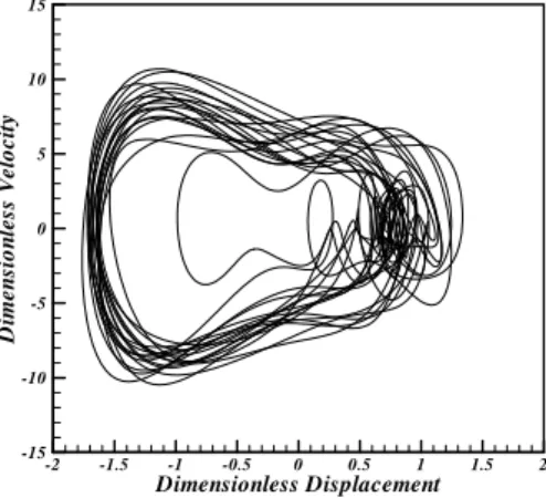
At zone C the plate motion is chaotic and the time history response and the related phase dia-gram at a specified condition (λ=420, n=0, Rx=Ry=8π2 is shown in Figs. 10 and 11, respectively.
Dimensionless Time
D
im
e
ns
io
nl
e
ss
D
is
p
la
c
e
m
e
nt
0 2 4 6 8 10
-2 -1 0 1 2
Dimensionless Displacement
Di
m
e
n
si
o
n
le
ss
V
e
lo
c
it
y
-2 -1.5 -1 -0.5 0 0.5 1 1.5 2
-15 -10 -5 0 5 10 15
Figure 11: Phase plane of the chaotic motion(λ=420, n=0, Rx=Ry=8π2)
As mentioned before, the limit cycle oscillation occurs in zone D. The deflection time history and the related phase diagram in this zone for two specified conditions are shown in Figs. 12 to 15. However, for moderate Rx as dynamic pressure increases, the periodic limit cycle oscillation changes
to the simple harmonic limit cycle oscillation.
Dimensionless Time
D
im
e
ns
io
nl
e
ss
D
is
p
la
c
e
m
e
nt
5 6 7 8 9 10
-0.8 -0.4 0 0.4 0.8
Figure 12: Time history of the panel (λ=195, n=, Rx=Ry=4π2)
Dimensionless Displacement
D
im
e
n
sio
n
le
ss
V
e
lo
c
ity
-1 -0.8 -0.6 -0.4 -0.2 0 0.2 0.4 0.6 0.8 1
Dimensionless Time
D
im
en
si
o
n
les
s
D
is
p
la
cem
en
t
8 8.4 8.8 9.2 9.6 10 -1
-0.5 0 0.5 1
Figure 14: Non-dimensional deflection (λ=280,n=inf, Rx=Ry=4π2)
Dimensionless Displacement
D
im
e
ns
io
nl
e
ss
V
e
lo
c
it
y
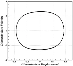
-0.8 -0.4 0 0.4 0.8 -4
-2 0 2 4
Figure 15: Phase plane (λ=280, n=inf, Rx=Ry=4π2)
5 CONCLUSIONS