www.biogeosciences.net/7/257/2010/
© Author(s) 2010. This work is distributed under the Creative Commons Attribution 3.0 License.
Biogeosciences
Process-based simulation of seasonality and drought stress in
monoterpene emission models
R. Grote1, T. Keenan2, A.-V. Lavoir3, and M. Staudt3
1Karlsruhe Institute of Technology, Institute for Meteorology and Climate Research (IMK-IFU), Kreuzeckbahnstrasse 19,
82467 Garmisch-Partenkirchen, Germany
2CREAF, Autonomous University of Barcelona (UAB), 08139 Bellaterra, Barcelona, Spain
3DREAM team, Centre d’Ecologie Fonctionnelle et Evolutive – Centre National pour la Recherche Scientifique
UMR 5175 (CEFE-CNRS), 1919 Rte de Mende, 34293 Montpellier Cedex5, France Received: 25 August 2009 – Published in Biogeosciences Discuss.: 11 September 2009 Revised: 29 December 2009 – Accepted: 5 January 2010 – Published: 20 January 2010
Abstract. Canopy emissions of volatile hydrocarbons such as isoprene and monoterpenes play an important role in air chemistry. They depend on various environmental condi-tions, are highly species-specific and are expected to be af-fected by global change. In order to estimate future emis-sions of these isoprenoids, differently complex models are available. However, seasonal dynamics driven by phenology, enzymatic activity, or drought stress strongly modify annual ecosystem emissions. Although these impacts depend them-selves on environmental conditions, they have yet received little attention in mechanistic modelling.
In this paper we propose the application of a mechanistic method for considering the seasonal dynamics of emission potential using the “Seasonal Isoprenoid synthase Model” (Lehning et al., 2001). We test this approach with three different models (GUENTHER, Guenther et al., 1993; NI-INEMETS, Niinemets et al., 2002a; BIM2, Grote et al., 2006) that are developed for simulating light-dependent monoterpene emission. We also suggest specific drought stress representations for each model. Additionally, the pro-posed model developments are compared with the approach realized in the MEGAN (Guenther et al., 2006) emission model. Models are applied to a Mediterranean Holm oak (Quercus ilex) site with measured weather data.
The simulation results demonstrate that the consideration of a dynamic emission potential has a strong effect on an-nual monoterpene emission estimates. The investigated mod-els, however, show different sensitivities to the procedure for determining this seasonality impact. Considering a drought impact reduced the differences between the applied models and decreased emissions at the investigation site by
approxi-Correspondence to:R. Grote
mately 33% on average over a 10 year period. Although this overall reduction was similar in all models, the sensitivity to weather conditions in specific years was different. We con-clude that the proposed implementations of drought stress and internal seasonality strongly reduce estimated emissions and indicate the measurements that are needed to further evaluate the models.
1 Introduction
Isoprenoids represent a heterogeneous compound class con-sisting of a wide range of reactive volatile hydrocarbons (i.e. isoprene, monoterpenes, and sesquiterpenes) which are emitted by most plant species. These emissions are highly important for air chemistry and air pollution (e.g. Fuentes et al., 2000; Kanakidou et al., 2005; Szidat et al., 2006; Ge-lencser et al., 2007), and are likely to indirectly affect the concentration of greenhouse gases (e.g. Pierce et al., 1998; Olofsson et al., 2005). Air pollution impacts depend on the availability of reaction partners, i.e. reactive nitrogen com-pounds, which have a regionally specific seasonal pattern that is driven by anthropogenic as well as biological activ-ities (e.g. Pierce et al., 1998; Fiore et al., 2005; Tie et al., 2006). Thus, it is not only the total amount but also the tim-ing of emissions that is important.
many regions, one of them being the Mediterranean basin (Giorgi et al., 2004; Giorgi 2006; Beniston et al., 2007; IPCC, 2007). It is thus expected that temperature is af-fecting short-term isoprenoid emission directly by enhancing biosynthesis and evaporation, but also indirectly by chang-ing boundary conditions on medium and longer time scales. These are particularly the dynamics of foliage development and enzymatic activities that are related to cumulative tem-perature (and others) and are known to affect emission (May-erhofer et al., 2005; Pio et al., 2005). Seasonal changes in emissions due to these two factors are termed as seasonal-ity throughout the following text. Seasonalseasonal-ity effects are re-ported for deciduous as well as coniferous species. Addi-tionally, environmental stresses, which also often follow a seasonal dynamic, such as drought, can alter the physiolog-ical pre-conditions for plant emission (Monson et al., 2007; Grote et al., 2009a). A better understanding of these seasonal dynamics is therefore also necessary for reliable projections of both current and projected future isoprenoid emissions.
The short-term emission of isoprenoids is a function of temperature and radiation and has been described as such by several models (see reviews in Arneth et al., 2007; Grote and Niinemets, 2008), which have been applied on local, regional and global scales. These models, however, have a develop-mental bias towards short term responses – partly due to a lack of long term seasonal measurement data. Other pro-cesses, operating over longer time scales, such as the effect of seasonality, the effect of seasonal cycles of water availabil-ity, and potential effects of CO2 fertilisation have received
little attention. Projected future atmospheric CO2
concen-tration changes have been suggested to modify the emission response on the decadal or longer time scale (Possell et al., 2005; Arneth et al., 2007, 2008a). The determination of sea-sonality and drought effects, however, has not as yet been systematically investigated, and still represents a major un-certainty of biogenic emission simulations (Funk et al., 2005; Monson et al., 2007; Arneth et al., 2008b; Keenan et al., 2009c).
The potential (or basal) emission is a species specific fac-tor (hereafter referred to as emission facfac-tor (EF)) that de-scribes emission rates under standard conditions (e.g. 30◦
C, 1000 µmol PAR m−2s−1). The isoprenoid emissions from
most models scale linearly with this factor which is known to change considerably during the year (e.g. Monson et al., 1994; Hanson and Sharkey, 2001; Hakola et al., 2006; Holzinger et al., 2006). The change in potential emission throughout the year is either neglected (particularly when only short periods are investigated) or empirically derived correction factors/equations are introduced (e.g. Staudt et al., 2000, 2002; Schaab et al., 2003; Keenan et al., 2009c). Al-though it is known that emission potential depends on pre-vailing temperature and light conditions (e.g. Staudt et al., 2003), only a few approaches have been developed to derive seasonality dynamically from environmental influences:
Fuentes and Wang (1999) used a function fitted to cu-mulated temperature or growing degree days, respectively, He et al. (2000) correlated emission potential to the num-ber of monthly sunshine hours, and Geron et al. (2000) ap-plied the integrated temperature of the previous 18 h instead of instantaneous temperature. However, there are only two models known to the authors that explicitly account for the cumulative effect of both impacts temperature and radiation, throughout longer time periods. One is the respective routine of the MEGAN model (Guenther et al., 2006; M¨uller et al., 2008), which applies an empirical adjustment based on the past 10 days of light and temperature to calculate emissions, and the other is the SIM model that derives the seasonal course of the isoprenoid forming enzyme activity, which is closely related to potential emission, explicitly from the pre-vious days climatic conditions (Lehning et al., 2001). Only the latter model reflects the finding that seasonal changes in enzyme activity result from physiological production and de-struction processes (Lehning et al., 1999; Loreto et al., 2001; Fischbach et al., 2002; Mayrhofer et al., 2005).
The second seasonal emissions driver is drought stress. Mild drought stress does not affect the light dependent emis-sion of isoprene and monoterpenes or reduces it only mod-erately (e.g. Bertin and Staudt, 1996; Brilli et al., 2007; Staudt et al., 2008). Strong, long-lasting drought, however, decreases isoprenoid emissions considerably (Hansen et al., 1999; Pegoraro et al., 2004, Lavoir et al., 2009). Overall, an impact of summer drought on annual isoprenoid emission has frequently been observed (Geron et al., 1997; Staudt et al., 2002; Plaza et al., 2005). A mechanistic understanding of isoprenoid responses to drought stress, however, has not yet been established. Due to this limited understanding as well as the strong dependence on species and site, drought effects have not yet been consistently represented in emission mod-elling.
In this paper, we investigate the sensitivity to drought stress and seasonality of three isoprenoid models commonly used in regional/global applications (GUENTHER, Guen-ther et al., 1993; MEGAN, GuenGuen-ther et al., 2006; and NI-INEMETS, Niinemets et al., 2002a), and one model of higher detail that has only been applied to specific sites and species (BIM2, Grote et al., 2006). We concentrate on the inves-tigation of light-dependent monoterpene emissions, whose emission behaviour is generally similar to that of isoprene (Ciccioli et al., 1997). Emissions from storages are assumed not to be relevant in the investigated ecosystem and are thus not accounted for. The models are compared on the basis of the same canopy model which is constrained through Eddy-flux data (Baldocchi et al., 2001; Misson et al., 2007) and the boundary conditions of a Mediterranean Holm oak stand (Quercus ilex). Emissions measurements, gathered on site, are used to calibrate the models.
seasonality procedure. Additionally, we suggest relations be-tween monoterpene emission and relative soil water avail-ability that are specifically adapted to each of the emission models.
2 Materials and methods
2.1 Site description and data availability
Data and simulations refer to a study site located 35 km NW of Montpellier (Southern France) in the Pu´echabon State For-est (3◦35′45′′E, 43◦44′29′′N, 270 m a.s.l.). Vegetation is
largely dominated by a dense over-storey of Holm oak ( Quer-cus ilex) trees (mean canopy height: 5.5 m, rooting depth down to 4.5 m). The climate is typical Mediterranean with cool and wet winters and warm and dry summers. The mean annual temperature is 13.5◦
C and the mean annual precipita-tion is 872 mm. Soil texture is homogeneous down to 0.5 m depth and can be denoted as silty clay loam (referring to the textural triangle, United States Department of Agricul-ture), with a limestone rock base. For more details on the site see http://www.cefe.cnrs.fr/fe/puechabon/. Eddy covari-ance fluxes were measured at a half hourly time step at a height of 11 m. The eddy covariance facility included a 3-dimensional sonic anemometer (Solent R2 during the 1998– 1999 periods and R3 since 2000, Gill Instruments Instru-ments, Lymington, UK) and a closed path infrared gas an-alyzer (IRGA, model LI 6262, Li-Cor Inc.), both sampling at a rate of 21 Hz. Flux data were processed following Aubi-net et al. (2000). An overview of the technical facilities can be obtained from the CarboEuroFlux network site at http: //www.bgc-jena.mpg.de/public/carboeur/sites/puechab.html. Due to the Mediterranean-type climate and the low wa-ter holding capacity, the wawa-ter content in summer falls reg-ularly below the value at which drought stress limitations to photosynthesis are expected (Rambal et al., 2003; Keenan et al., 2009b). The timing and extent of drought conditions varies from year to year, but water content values close to the wilting point are observed almost every year. For the years of measurements, 2005 was slightly cooler (annual average temperature 13.0◦
C) and 2006 warmer and dryer than the long-term average (total precipitation 773 mm, annual aver-age temperature of 14.1◦C, see Allard et al., 2008). The
period 1998 to 2007 that we used to compare the different emission models was slightly warmer and wetter than the long-term average (13.7◦
C, 913 mm). The standard devia-tions in this period are 0.6◦
C and 228 mm, respectively. The investigation of well-watered trees has been carried out at a 10-year old Holm oak plantation which was irri-gated regularly during 2006. This plantation is located in Montpellier close to the CEFE-CNRS institute in southern France (43◦
36′
N, 5◦
53′
E) on a deep clay soil with good water availability. Genetic similarity of the trees to those of the eddy-covariance measurement site is ensured because
the trees originate from acorn samples from the same site (Pu´echabon State Forest). Since only measurements of new leaves are used for fitting the emission potential of the mod-els, stand structural aspects are not important. Due to the close vicinity of both sites that are only app. 30 km apart, we assume no difference with respect to their atmospheric climate conditions.
Measurements of leaf scale emissions are taken from Grote et al. (2009a) and Lavoir et al. (2009). They had been conducted from May to October (12 occasions in 2005, 9 oc-casions in 2006) on the field site Pu´echabon at current year leaves of adult trees about every second week under sun-lit conditions (mostly between 10 and 12 am). Three trees per occasion had been sampled. Identical measurements had been carried out in 2006 at the irrigated plot in Montpellier during the weeks in between (9 occasions). All measured leaves (3 per occasion) from 2006 had also been used for the enzyme analyses.
Enzyme activity has been determined in 2006 according to standard protocols described in Fischbach et al. (2000) using the same leaves as used for emission measurements. Enzy-matic data provide calibration information for the seasonal dynamics model SIM. The emission measurements from the irrigated plot (only 2006) are used to calibrate the combined SIM/ emission models (without drought stress). The emis-sion data from the natural field site (2005 and 2006) are then used to evaluate the results from simulations that included drought stress (= relative soil water depletion). Although drought stress acts differently on the GUENTHER and NI-INEMETS models, no model-specific fitting has been carried out. BIM2 relies on previous calibration based on a smaller data set (Grote et al., 2009a). For both years half-hourly weather input data was available. Long term comparisons are based on hourly weather data from 1998 to 2007. In or-der to investigate the sensitivity of the models to drought and seasonality, we ran different simulation experiments which considered:
1. a fixed emission factor with no drought stress, 2. a fixed emission factor with drought stress,
3. a seasonally dynamic emission factor with no drought stress and,
4. a seasonally dynamic emission factor including drought stress.
2.2 Model description
2.2.1 Modelling framework
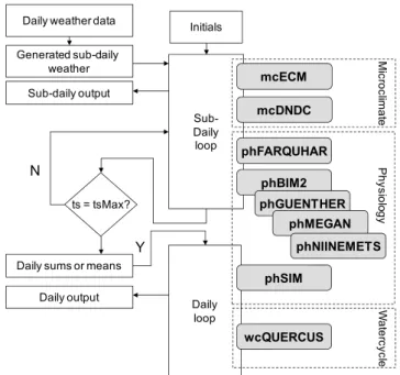
For all simulations, a modelling framework has been used which is designed to couple one-dimensional biosphere mod-els to describe different processes within the ecosystem. The framework provides climate data and initial variables for ev-ery (below- and aboveground) layer of the ecosystem based on initial site information and climate input data. This en-sures the same initial conditions and dynamic boundary con-ditions for all emissions models in the investigation. Short-timestep model results are aggregated in order to be used as input for models with larger time steps. The models imple-mented can be applied alternatively or in addition to each other (for more information see Grote, 2007; Grote et al., 2009a, b; Holst et al., 2010).
In the current context the short-term isoprenoid emis-sion models MEGAN (Guenther et al., 2006), GUENTHER (Guenther et al., 1993), NIINEMETS (Niinemets et al., 2002a), and BIM2 (Grote et al., 2006) are coupled with mod-els describing the canopy micro-climate within the canopy (ECM, Grote et al., 2009a) and the soil (DNDC, Li et al., 1992), photosynthesis (FARQUHAR, Farquhar and Von Caemmerer, 1982), phenology (SIM, Lehning et al., 2001; Grote, 2007), and soil hydrological conditions (QUERCUS, Rambal et al., 1993, 2003) (see Fig. 1 and model descrip-tions below). The seasonal development of enzyme activ-ity and basal emission factors for all emission models but MEGAN are calculated as an addition of the SIM model ap-proach (Lehning et al., 2001), The photosynthesis and emis-sion models are run on a half hourly time step, correspond-ing to the available weather data. The boundary conditions for emissions, i.e. enzyme activities or basal emission fac-tors, leaf development states, and the state of relative water supply are updated daily.
2.2.2 Biosphere models
ECM (empirical canopy model) calculates radiation, tem-perature, vapour pressure, and wind profiles for a given canopy. The radiation regime is determined using a simple one-dimensional light extinction scheme based on canopy layers with fixed extension and empirical foliage distribution (Grote, 2007). The sunlit and shaded fractions of the foliage are differentiated for each layer (Spitters et al., 1986). Tem-perature development in the canopy is given by an empirical function for each layer between the canopy upper boundary and at the soil surface. Soil surface temperature is calculated by the DNDC (DeNitrification-DeComposition) module (Li et al., 1992) on the basis of heat capacity and conductance of the soil components in each soil layer.
FARQUHAR: The common Farquhar approach (Farquhar and Von Caemmerer, 1982) is used along with the parame-terization provided by Long et al. (1991). Stomata
conduc-W
a
te
rcycl
e
Daily loop Sub-Daily loop
P
h
y
s
io
lo
g
y
Generated sub-daily weather
phBIM2 Sub-daily output
phFARQUHAR
phSIM
wcQUERCUS ts = tsMax?
N
Y
Daily weather data
Daily output
Initials
Daily sums or means
mcDNDC mcECM
M
ic
ro
c
lim
a
te
phGUENTHER phMEGAN
phNIINEMETS
Fig. 1.Model framework. The three modules BIM2, GUENTHER,
and NIINEMETS are alternatively called together with the other modules that describe the boundary conditions for isoprenoid emis-sion, i.e. microclimate, physiology (photosynthesis and foliage de-velopment), and soil water content. The MEGAN model is in the same module as the GUENTHER model but with additional options to account for the integrated temperature and radiation effects.
tance is calculated with the approach suggested by Ball et al. (1987). Photosynthesis is calculated separately for sunlit and shaded foliage but pooled over each layer for emission input. This is in accordance with the determination of emis-sion activity which is also layer specific.
Drought stress is accounted for by the stomata conduc-tance calculations inherent in the model and additionally by means of a reduction in the rate of electron transport and maximum carboxylation capacity (Vcmax) (Keenan et al.,
2009b). Here we apply a simple linear relation to relative soil water content (RWC), parameterised from measurements of stomata conductance (Rambal et al., 2003):
DS=min
1.0, RWC
RWClim
(1) with DS denoting the drought stress scaling factor. The limit value of relative soil water content at which drought stress starts to effect a process (RWClim) has been set to 0.7
(Ram-bal et al., 2003; Keenan et al., 2009b).
fixed to a value of 1.1) that accounts for a variable propor-tion of ground heat flux in dependence on leaf area index (LAI) and vegetation density. Transpiration is determined from potential evapotranspiration and foliage conductance in half hourly time steps using air temperature and solar irradi-ation as input. The model has already accurately represented the soil water content throughout the years 1993 to 2006 at the Pu´echabon site (see Grote et al., 2009a).
2.2.3 Emission models
Three commonly used emission models of varying complex-ity were coupled to the biosphere modelling framework.
GUENTHER/MEGAN: By far the most widely used model for simulation of natural isoprenoid emissions is de-veloped by Guenther et al. (1991, 1993). This approach describes the emission rates using potential emission fac-tors for isoprene (EFI)and monoterpenes (EFM), and
ad-justing these potentials by two empirical factors, one de-scribing the response to light intensity and the other to leaf temperature. The correlation between short term fluctua-tions, light intensity and leaf temperature is widely studied and much work has gone into validating the GUENTHER model under different environmental conditions (e.g. Mon-son et al., 1994; Petron et al., 2001). The emission fac-tors used in the model are emission rates normalized to a leaf temperature (T) of 30◦
C and quantum flux density (Q) of 1000 µmol m−2s−1photosynthetic active radiation (PAR)
(Guenther, 1991; Guenther et al., 1993, 1995, 1997). For more information, we refer to the detailed descriptions in these papers.
In the original Guenther model, several coefficients that describe the dependency to light and temperature are fixed parameters. In the MEGAN emission model, these values are dynamic in time and depend on short term (24 h) and long term (10 days) fluctuations in temperature and light inten-sity (see Guenther et al., 2006). Additionally, the sunlit and shaded parts of the foliage within one canopy layer are pa-rameterised differently, representing their sensitivity to light. These algorithms are applied for all simulations indicated as the MEGAN model, whereas SIM is not used. Other speci-fications of the MEGAN model are not considered which is possible because we apply the model to an evergreen canopy (in this case no leaf age factor is considered in MEGAN).
NIINEMETS: This model (Niinemets et al., 2002a) for isoprene and monoterpene emissions takes a more process-based approach. It links the emission rates to synthase en-zyme activity (SS)to predict the capacity of isoprenoid
syn-thesis as well as to foliar photosynthetic metabolism via the photosynthetic electron transport rate,J, to predict substrate (Niinemets et al., 1999; Niinemets et al., 2002a). The supply of dimethylallyl-pyrophosphate (DMAP) and nicotinamid-dinucleotid-phosphate (NADPH), which both depend on the rate of photosynthetic electron transport, are considered to be the main controlling factors.
Emission rates are calculated from the fraction of total electron flow that is used for isoprenoid synthesis, the rate of photosynthetic electron transport, and the cost of isoprenoid synthesis in terms of electrons. Thus, emissions are closely linked to photosynthetic activity of leaves using only one single leaf dependent parameterε, the fractional allocation of electron transport to synthase activity. Emission rates are given by the equation (Niinemets et al., 1999; Niinemets et al., 2002a):
E=εJT
Ci−Ŵ∗
ς (4Ci+8Ŵ∗)+2(Ci−Ŵ∗)(ϑ−2ς )
(2) whereJT is the total rate of photosynthetic electron
trans-port, Ci is the internal CO2 concentration, and Ŵ∗ is
the hypothetical CO2compensation point of photosynthesis
that depends on photorespiration (Farquhar and Von Caem-merer, 1982). ς is the carbon cost of specific isoprenoid (6 mol mol−1 for isoprene and 12 mol mol−1 for
monoter-penes) and ϑ is the NADPH cost of specific isoprenoids (mol mol−1). For monoterpenes,ϑ is found as a weighted
average of the costs of all terpene species emitted. In practice,ϑ ∼=28 mol mol−1, with small variability because
the contribution of oxygenated monoterpenes that may have lower electron cost or reduced monoterpenes that may have higher electron cost is generally small (Niinemets et al., 2002a, 2004). ε, the fractional allocation of electron trans-port to isoprenoid synthesis, is given by:
ε=Fd SS Jmax
(3) whereSs is the specific activity of isoprenoid synthase
(ei-ther isoprene or monoterpene synthase) in mol isoprenoid (g isoprenoid synthase)−1s−1that depends on temperature
ac-cording to an Arrhenius type equation that has a temperature optimum, andJmaxis the light saturated rate of total electron
transport that scales with temperature in a similar manner (Niinemets and Tenhunen, 1997). Fd (g m−2mol electrons
mol isoprenoid−1) is the scaling constant that depends on
isoprenoid synthase content (g m−2) and also converts from
isoprenoid units to electron transport units (mol isoprenoids mol electrons−1) (Niinemets et al., 1999, 2002a). Thus, light
dependence of isoprenoid emission entirely results from the light effects on photosynthetic electron transport, while tem-perature dependence is a combined temtem-perature response of isoprenoid synthase and electron transport activities.
biosynthesis-related enzymes (i.e. isoprene and monoterpene synthases). Primary substrates for the emission model are provided by photosynthesis (Grote et al., 2009a). The emis-sion model uses a fixed internal time step of seven seconds. To mitigate the impact of the different time steps between photosynthetic supply and usage, the supply rate is adjusted to continuously increase or decrease between two consecu-tively following assimilation rates.
The immediate substrates for isoprenoid formation PEP (phosphoenolpyruvate) and PGA (phosphoglycerate) are as-sumed to be smaller than the photosynthetic production of triose phosphates (tp), considering exchange equilibrium caused by import and export from the plastids and trans-formation of triose-phosphate into larger molecules such as starch. The integrated effect is seen as an equilibrium rela-tion to photosynthetic producrela-tion:
PGA=FPGA· tp
2
KMtp
+tp (4)
PEP=(1−FPGA)· tp
2
KMtp+tp
(5)
KMtp (Michaelis-Menten constant for triose-phosphate
re-moval) and FPGA (fraction pga of whole available triose-phosphates) are empirical determined parameters (units in µmol L−1). The relation had been set a priori to 0.375
based on unpublished measurements (Schnitzler, personal communication, 2006). The value is difficult to find in lit-erature for tree species. For crops it has been reported to be between app. 0.5 and 0.9 (e.g. Labate et al 1990; Henkes et al, 2001). However, sensitivity tests show that emission re-sults are hardly sensitive to this ratio (rere-sults not presented). KMtpis estimated to be 100 (see also Grote et al., 2009a).
The concentration of intermediates declines because of use for transformation into higher molecules and transport into other plant compartments. These processes may have numer-ous environmental dependencies which are not well known and thus are not explicitly considered here. Instead we make the reasonable assumption that the “leaching” of assimilates depends on its concentration and is not directly dependent on production rate. Thus the concentration declines when the “outflow” is larger than the “inflow”, provided by pho-tosynthesis. This is the case during conditions where photo-synthesis is severely reduced, i.e. during the night or extreme drought. This is simply described by:
c′
i=ci−LRi·t s·ci (6)
wheretsdenotes the time step (7 s) and c is substrate con-centration (µmol,L−1). Subscript i denote the substrates
(PGA, PEP, NADPH, and adenosine-triphosphate [ATP]) as well as the intermediates of the MEP pathway to isoprene and monoterpene production. LR is the loss rate set to the same value for PGA, PEP, and all intermediates. Loss rate has been derived iteratively by fitting BIM2 to the measured
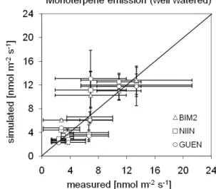
Fig. 2. Simulated and measured leaf scale monoterpene emissions
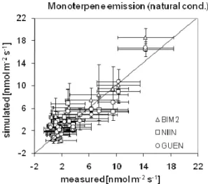
at selected dates in 2006 from sunlit leaves of the well watered Holm oak site. Three models (BIM2, NIINEMETS, GUENTHER) are applied using SIM based seasonality. Each data point repre-sents three leaf-measurements from a separate tree each. The error bars represent the standard deviation of measurements and simula-tions for three measurements (one per tree) that were carried out per measurement day.
emissions of the well watered plants (Grote et al., 2009a; see Fig. 2). The approximation has been carried out by changing the value in steps of 0.0005 µmol µ mol−1s−1with the aim to
obtain concentrations of GDP that are similar to those mea-sured by Nogues et al. (2006) in Q. ilexchloroplasts. The resulting value is 0.0035 µmol µmol−1s−1. The loss rates
of ATP and NADPH molecules are set 10-fold the value of other molecules to obtain realistic concentrations (Loreto and Sharkey, 1993; Nogues et al., 2006).
2.2.4 Drought impacts in emission models
Drought impacts on emissions are realized either directly by reducing the emission process itself, or indirectly by the ef-fect of a reduced photosynthesis. Further indirect impacts, e.g. due to changes in leaf temperature when transpiration is reduced are currently not considered.
The same drought stress formulation determines the re-sponse of the NIINEMETS model, but the effect is indirect because not emission itself but the rate of electron transport (JT) and Vcmax are reduced by Eq. 1. Since both
photo-synthetic variables determine the emission capacity, drought stress leads to reduced emissions.
In the BIM2 model, the effect is also indirect because none of the variables used to describe the emission process itself are affected by soil water availability. The impact is solely due to a lack of precursor availability, which is controlled by photosynthetic production and depletion of emission precur-sors by various processes.
2.2.5 Emission enzyme activity and emissions potentials
All other factors being equal, simulated emissions scale lin-early with the species specific emission, represented by the emission factor EF. EF has been found to exhibit strong sea-sonal variation, though this variation has not yet been ex-plained in a process based manner. The SIM model provides a mechanistic description of this seasonal variation, relating the emission potential to temperature and radiation driven en-zyme dynamics.
The SIM model is a simple algorithm that derives daily enzyme activity from the previous day’s value, an increas-ing and a decreasincreas-ing term. The increase is defined by the daily radiation sumI (Jcm−2), an Arrhenius term based on
daily average temperature,T (◦K), and the relative
develop-ment state of the leaves, pstat, whilst the decrease is a con-stant fraction of the previous days enzyme activity. Thus the change in enzyme activity for a particular day and canopy layer can be written as:
1act
dt =α0·pstat·I·arrh−µ·act, (7)
arrh=A·e
−Eact
R·T
(8) where act is the enzyme activity of the previous day (µmol L−1s−1),Rthe general gas constant (8.3143 J mol−1), α0 the enzyme formation term (s−1), µ the enzyme decay
term (0.175 s−1)(Lehning et al., 2001),Aa unitless factor
for normalizing the Arrhenius term to 1 at 30◦
C (660.1E6), andEact, the activation energy for a doubling of the
reac-tion velocity (51164.8 J mol−1). Emission activity is
cal-culated for each canopy layer separately (nmol m−2 foliage
s−1). The leaf development term pstat indicates the
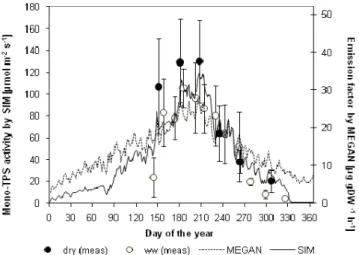
pheno-logical state of the leaf according to Lehning et al. (2001) and Grote (2007). It increases from 0 to 1 during the period of flushing and decreases with age after senescence has started. The monoterpene synthase formation term,α0, is adjusted to
measurements taken on site (see Fig. 3).
Enzyme activity is transformed to the emission factor us-ing the specific leaf weight (LSW), which changes linearly with canopy depth from 233 g m−2 at the upper canopy
Fig. 3. Seasonal development of monoterpene activity
measure-ments (from both dry and well-watered (ww) trees) and estimated emission factors (for MEGAN and SIM) for the year 2006 (repro-duced from Grote et al. 2009a) together with the effective emission factor for the MEGAN model presented on the left y-axis (see text for further information).
boundary to 100 g m−2 at the bottom of the canopy
(Ni-inemets et al., 2002b). For the GUENTHER approach, EF (µg g−1dry weight h−1)is given by:
EF= act ·2
LSW·FSC
(9) The transformation term2is 120×3.6, which is the mo-lar mass of carbon atoms within one monoterpene molecule times the transformation from nmol s−1into µmol h−1. F
SC
is a factor that accounts for the fact that the enzyme activity reflects a state that is substrate saturated which is never the case and thus has to be reduced to reflect the emission factor. It is adjusted based on the measurements from well watered plants (see below). Similarly, Eq. 7 is also used to derive the basal emission factor for the NIINEMETS approach,Eact
(µmol g−1dry weight s−1). The value of2here is 0.01,
cor-responding to the unit conversion from nmol to µmol C con-sidering 10 carbon atoms in one monoterpene molecule.
For the GUENTHER and NIINEMETS models we cali-brated the scaling factor (FSC)to the same data (obtained
under well watered conditions) in order to approach the 1:1 line for each model separately (see Fig. 2). This resulted in anFSCvalue of 5.2 for the GUENTHER and 7.7 for the
NI-INEMETS model (regression r2 values are 0.74 for BIM2 and GUENTHER, and 0.62 for NIINEMETS; standard er-rors are 2.08, 2.86, and 2.26 for BIM2, GUENTHER and NIINEMETS, respectively).
In order to compare the effect of the seasonality in the three model approaches, simulations are additionally run with a fixed emission factor of 28 µg gDW−1h−1 (Seufert
0 0.2 0.4 0.6 0.8
0 50 100 150 200 250 300 350
G
PP [m
o
l
m
-2
da
y
-1]
Day of the year
simulated
measured
y = 0.928x R² = 0.498 0
0.2 0.4 0.6 0.8
0 0.2 0.4 0.6 0.8
sim
u
la
te
d
measured
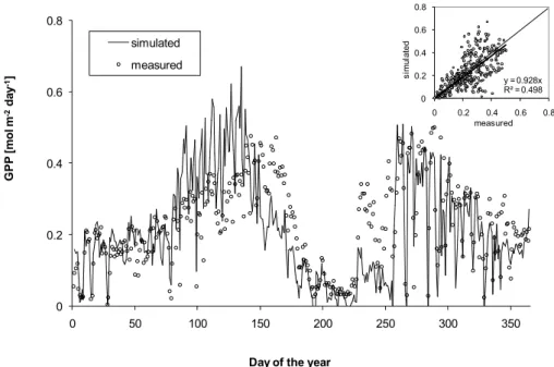
Fig. 4.Simulated and measured gross primary production (GPP) during the year 2006.
Staudt et al. (2002) and Lavoir et al. (2009). The value has been transformed into enzyme activity using the reciprocal of Eq. 7. Additionally, the MEGAN model is run for compari-son using the fixed emission factor and the internal modifica-tion of variables (see above). The representamodifica-tion of season-ality in the MEGAN model is derived from emission result-comparisons of MEGAN and GUENTHER models. This is demonstrated in Fig. 3 showing the relation of MEGAN and SIM algorithm output.
2.2.6 Simulated boundary conditions and other model constraints
For scaling from leaf to canopy we used assumptions on foliage distribution as outlined in Grote (2007). These are based on measurements of Sala et al. (1994) that show a highly skewed foliage distribution with more than 90% of the total leaf weight concentrated in the upper 30% of the canopy. Also, phenological development has been accounted for as described in Grote (2007) considering a variation of leaf area index between 2 and 3.5 with the minimum in spring and the maximum in early summer.
The ECM model calculations of microclimate are dis-cussed in Grote et al. (2009a). They show distinct radiation absorption averaging to 80% light reduction within the upper half of the canopy but only small variation in temperature (app.+/−1 degree between upper and lower canopy layers during typical summer days).
To evaluate simulated photosynthesis at the canopy scale we used data of a continuously measuring flux tower at the Pu´echabon site that also provided climatic boundary data (averages 1998–2006 are presented in Allard et al., 2008).
This tower is part of the CarboEurope network (see Bal-docchi et al., 2001; BalBal-docchi, 2003). The correlation be-tween simulations and measurements is reasonably good de-spite occasional mismatches that are caused by mechanisms not covered in the modelling approach, e.g. there was prob-ably and insect induced foliage loss in spring 2006. The smaller amount of foliage decreased GPP and is a likely rea-son for an over-estimation of GPP during this time and an over-estimation of drought stress (under-estimation of GPP) during early summer (Fig. 4).
The soil water content calculated daily by the QUERCUS model has been successfully evaluated for the Pu´echabon site (Rambal et al., 2003; Grote et al., 2009a) for the period from 1998 to 2006.
3 Results
3.1 Monoterpene emission at leaf scale
First, we compare the measured leaf scale emissions from the drought stressed Pu´echabon site with simulation results from the same time periods (Fig. 5). This is done similarly as described for calibrating theFSCfactor of the NIINEMETS
Fig. 5.see Fig. 2 but for drought stressed site and including measurement occasions in 2005 and 2006.
3.2 Stand scale monoterpene emissions
3.2.1 Diurnal effect
Seasonal and annual model differences originate from the sum of daily emissions which are characterized by their peak amount (usually during midday), the development of emis-sion during the day, and the distribution within the canopy. While it could be shown that the midday emission rate of sunlit leaves is more or less well represented, particularly under well watered conditions (Figs. 2 and 3, Grote et al., 2009), no data are available to evaluate emission from leaves within the canopy or during morning and afternoon periods. Thus, it is important to show why models that are evaluated with the same short-term data may produce different emis-sion sums when longer time periods and the whole canopy are considered.
While differences between models in the sunlit part of the canopy are small (Fig. 6a and b), they are particularly ob-vious during the drought stress period in the shaded part of the canopy (Fig. 6d). Here, the NIINEMETS model simu-lates approximately 2-fold higher emissions than the GUEN-THER model and 5-fold higher emissions than BIM2. This reflects that the indirect drought response implemented for the NIINEMETS approach is less sensitive to severely lim-ited water supply than the direct response function used for the GUENTHER model. It also shows the particular sensi-tivity of BIM2 to carbon supply which is decreased by the combined shading and drought impacts.
Other differences are less clear or might cancel out dur-ing the day. For example the NIINEMETS model generally simulates a steeper increase of emission in the early hours be-cause only small photosynthetic activities are needed to sup-port monoterpene production. Furthermore, the dependency on photosynthesis in the NIINEMETS and BIM2 approaches
enable higher emission rates in the afternoon, particularly in the shaded canopy part, when the decreasing light availability already leads to a steep decrease in emissions simulated by the GUENTHER model (Fig. 6c). It should also be noted that in very occasional cases (hot, no clouds, no drought stress) emission simulation in NIINEMETS and BIM2 (but not in GUENTHER) can be slightly affected by a photosynthetic decline due to stomatal midday depression (days 180, 181). 3.2.2 Seasonality effect
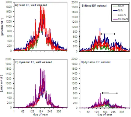
The differences in seasonality between the models are demonstrated in Fig. 7 and Table 1. Without drought all models simulate highest emissions in the summer (35–50% of the annual emission, Fig. 7c). However, summer drought strongly reduces emissions in all models leading to overall similar total emissions in spring and summer despite the tem-perature differences (Table 1).
The most obvious difference between models is apparent between MEGAN and the models driven by the SIM algo-rithm: MEGAN produces higher spring emissions due to its higher EF during this period (Fig. 3). However, the model is more sensitive to high temperature periods despite a similar EF, leading to faster in- and decreases.
Comparing the models that use the SIM algorithm, the NI-INEMETS model simulates relatively high emissions under low light and temperature conditions while it is less sensitive to environmental changes when these conditions are already good. Thus, emission rates are generally higher than those calculated by GUENTHER and BIM2 in winter, spring and autumn but smaller in summer as long as the drought im-pact is neglected (Fig. 7a and c). However, as discussed in the next paragraph, the NIINEMETS model (in its presented implementation) is also the least sensitive to drought stress, leading to higher (less decreased) emissions than those cal-culated with the other two models in summer under natural conditions (Fig. 7b and d).
Fig. 6.Diurnal simulated emissions using BIM2, NIINEMETS, and GUENTHER models at selected dates in 2005(A, C)and 2006(B, D)
for upper and mid canopy locations. Note the different scaling of y-axis.
0 200 400 600 800 1000 1200 1400 1600 1800 2000
B) fixed EF, natural BIM2
NIIN
GUEN
MEGAN
0 200 400 600 800 1000 1200 1400 1600 1800 2000
1 62 123 184 245 306
day of year D) dynamic EF, natural 0
200 400 600 800 1000 1200 1400 1600 1800 2000
[
μ
mo
l m
-2
d
-1]
A) fixed EF, well watered
0 200 400 600 800 1000 1200 1400 1600 1800 2000
1 62 123 184 245 306
[
μ
mo
l m
-2
d
-1]
day of year C) dynamic EF, well watered
Fig. 7.Simulated daily emissions of the year 2006 based on Pu´echabon site information with:(A)a fixed emission potential factor (EF) and
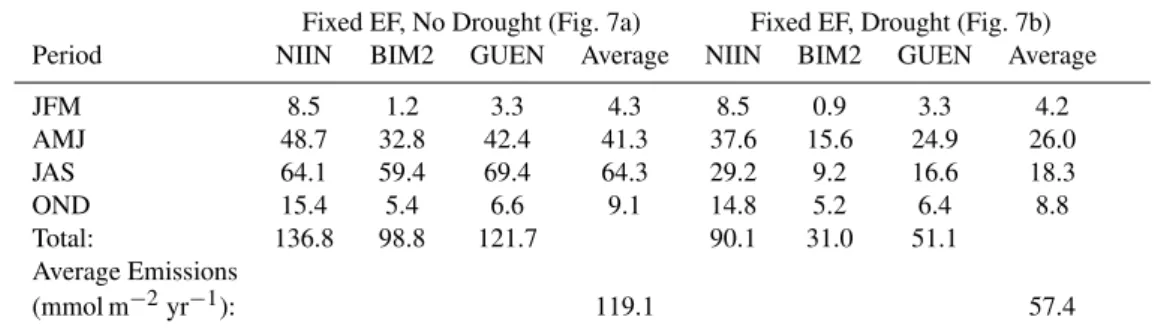
Table 1. Emissions totals (mmol m−2) for the periods JFM (January, February, March), AMJ (April, May, June), JAS (July, August,
September), and OND (October, November, December) for the four experimental set ups, for each model, at the Puechabon site in 2006. “Average emissions (mmol m−2yr−1)” refers to the average annual emissions from the three models for a particular experimental setup. EF
refers to the basal emissions factor. Values correspond to Fig. 7.
Fixed EF, No Drought (Fig. 7a) Fixed EF, Drought (Fig. 7b) Period NIIN BIM2 GUEN Average NIIN BIM2 GUEN Average
JFM 8.5 1.2 3.3 4.3 8.5 0.9 3.3 4.2
AMJ 48.7 32.8 42.4 41.3 37.6 15.6 24.9 26.0
JAS 64.1 59.4 69.4 64.3 29.2 9.2 16.6 18.3
OND 15.4 5.4 6.6 9.1 14.8 5.2 6.4 8.8
Total: 136.8 98.8 121.7 90.1 31.0 51.1
Average Emissions
(mmol m−2yr−1): 119.1 57.4
Table 1.Continued.
Dynamic EF, No Drought (Fig. 7c) Dynamic EF, Drought (Fig. 7d) Period NIIN BIM2 GUEN MEGAN Average NIIN BIM2 GUEN MEGAN Average
JFM 0.6 0.1 0.3 1.1 0.5 0.6 0.1 0.3 1.1 0.5
AMJ 16.6 19.9 15.9 26.3 19.7 11.5 8.7 8.1 14.4 10.7
JAS 34.2 49.5 40.7 50.5 43.7 14.6 6.8 9.5 11.9 10.7
OND 2.0 1.7 1.0 2.4 1.8 2.0 1.6 1.0 2.3 1.7
Total: 53.5 71.2 57.9 80.2 28.7 17.3 18.9 29.7
Average Emissions
(mmol m−2yr−1): 65.7 23.7
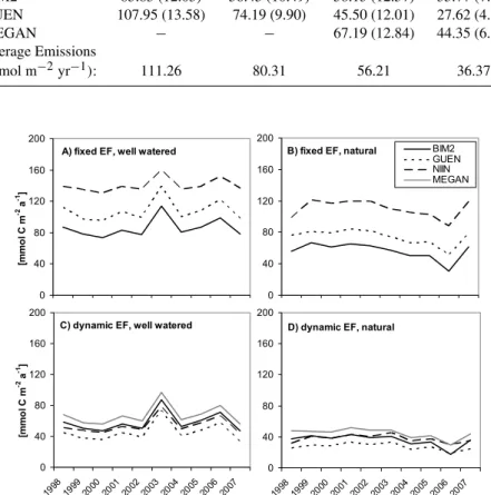
different models but also between different years are further reduced by drought stress (Fig. 8d). The negative drought impact on emission compensates (year 2003) or overcom-pensates (year 2006) the higher emissions due to the warm temperatures in these years.
The correlation of annual total emissions to annual max-imum temperatures is better than that to annual mean tem-peratures. It is also slightly negative to GPP (data not shown) which indicates that temperatures in summer are un-favourable for production even if drought stress is not con-sidered.
3.2.3 Drought stress effect
In 2006, in which the most intense drought of all investigated years occurred, photosynthesis as well as simulated emission starts to decline at day 156 when relative water content de-creases below a value of 40% (Fig. 7b and d) and recovers only in late summer (day 256). The additional drop in emis-sions around day 220 is associated with a temperature decline from app. 24 to 18 degrees (daily average). This has not been accompanied with a lot of rainfall so that drought stress is not mitigated. Scaled across the whole canopy, annual emission in 2006 is only between 24 (BIM2) and 45 (NIINEMETS) %
of that calculated for unstressed conditions. On average over the 10 year period, simulated annual emissions are reduced between 28 and 36% (Table 2). Monoterpene emissions un-der Mediterranean conditions are more closely correlated to water availability than to primary production or average tem-perature in all models. The sensitivity, however, is largest in BIM2, leading to particular low simulated emissions in 2006 despite producing otherwise similar results as those of the NIINEMETS model (−5%) and moderately smaller values than the GUENTHER model (−29%). The MEGAN model produces higher emission estimates than the other models (+34%). This reflects the fact that MEGAN contains an em-pirical measure of seasonality that is not as strong as that rep-resented by the SIM calculations (see Fig. 2) and thus leads to higher emissions particularly outside the dry period in spring and autumn (Fig. 7c and d).
Table 2.Average and standard deviation (shown in brackets) of annual emissions (mmol m−2yr−1)for each model for the four experimental
setups at the Puechabon site over the period 1998–2007. “Average emissions (mmol m−2yr−1)” refers to the average annual emissions from all models for a particular experimental setup. EF refers to the basal emissions factor. Values correspond to Fig. 8.
Fixed EF, Fixed EF, Dynamic EF, Dynamic EF, Period No Drought Drought No Drought Drought 1998–2007 (Fig. 8a) (Fig. 8b) (Fig. 8c) (Fig. 8d)
NIIN 140.01 (8.83) 110.29 (11.11) 54.01 (10.72) 37.75 (4.90) BIM2 85.83 (12.03) 56.45 (10.49) 58.13 (12.57) 35.77 (7.42) GUEN 107.95 (13.58) 74.19 (9.90) 45.50 (12.01) 27.62 (4.50)
MEGAN − − 67.19 (12.84) 44.35 (6.35)
Average Emissions
(mmol m−2yr−1): 111.26 80.31 56.21 36.37
B) fixed EF, natural
0 40 80 120 160 200
1998 199920002001 200220032004200520062007 BIM2 GUEN NIIN MEGAN
D) dynamic EF, natural
0 40 80 120 160 200
19981999200 0
2001200 2
200 3
2004200 5
2006 2007
A) fixed EF, well watered
0 40 80 120 160 200
19981999 20002001 2002 2003 200420052006 2007
[mm
o
l C
m
-2 a -1]
C) dynamic EF, well watered
0 40 80 120 160 200
199819992000 2001200220032004200520062007
[mm
o
l C
m
-2 a -1]
Fig. 8.see Fig. 7 but simulated annual emissions for the period of 1998 to 2007.
4 Discussion
4.1 Seasonal and within canopy variations
The results demonstrate the potential importance of consid-ering the seasonality of emission dynamics. This corrobo-rates the findings of many authors before (e.g. Monson et al., 1994; Tarvainen et al., 2005; Holzinger et al., 2006; Hakola et al., 2006; Dominguez-Taylor et al., 2007). We have pre-sented a general process-based solution that computes this seasonality from temperature and light conditions which is applicable to at least the most common emission models used today in regional to global applications, be they empirical or more process-based. However, it remains to be investigated to which degree the approach can be applied with regard to species-dependent or plant-functional type related parame-ters.
temperature development as the GUENTHER model. This is attributed to the fact that emissions additionally depend on photosynthetic substrate supply which is sometimes limiting even under non-stressed conditions, particularly in deeper canopy layers.
Unfortunately, measurement availability is very limited (see Pacifico et al., 2009). It should be considered that past model studies on biogenic emissions have reported to be most sensitive at high temperatures and radiation values (Arneth et al., 2007, Keenan et al., 2009a). This suggests that model differences will probably be larger at more south-ern locations. Our results therefore represent something of an upper range of model differences due to temperature and light with respect to the time scale included in the study.
The comparison with the MEGAN model shows that sea-sonality is less expressed than with the SIM approach. Due to limited evaluation data, we cannot judge which model is “better”. Also the absolute emission values obtained should be interpreted with care because the leaf-scale emission fac-tor used in this study is determined on sun-lit leaves and is not the same as the “canopy emission factor” used in MEGAN that already takes into account a variation through-out the canopy. It is however assumed that introducing a leaf age factor also to evergreen canopies would bring the MEGAN approach closer to the one applied in SIM. In any case, the finding should encourage further investigations into the matter and indicates that seasonality settings may not eas-ily be transferred between species and regions.
Overall, the application of the SIM algorithm for the cal-culation of emissions potentials provides a method through which seasonal variation of the basal emission factor (or ac-tivity) can be accounted for. Higher temperatures in the fu-ture could alter the seasonal cycle of enzyme activity, which may increase the emissions potential, in particular during spring and autumn, where temperature is currently a limit-ing factor. Increased enzyme activity could lead to increased emissions in the future, a fact that is currently not included with mechanistic detail in any large scale emissions model estimates. The advantage of an activity-based description in comparison to an empirical one is in particular that it can be more easily evaluated. Our example simulations indicate that the SIM mechanism results in smaller and less variable spring and autumn emissions in the Mediterranean area than the standard-MEGAN procedure. This dependence of en-zyme activity on the temperature and radiation regime also implies a differentiation of species emission potentials over a climatic gradient, which may explain the reported regional variation in emissions potentials (Guenther et al., 2006) and the generally large variability in reported emission potentials in the literature. The implication of the SIM model may thus provide a mechanistic means of describing regional changes in emissions potentials, but more data is required to reach a conclusive decision.
Due to the dependence of enzyme activity on the temper-ature and radiation regime, long-term dynamics in depen-dence on environment also leads to a spatial differentiation of emission factors within the canopy. This corresponds to results from Geron et al. (1994) and Harley et al. (1996) which indicate that the emission capacity varies with canopy depth. In Western Hemlock emission potentials in different canopy heights were significantly different although this was not found in Douglas fir forests (Pressley et al., 2004).
4.2 Drought stress effect
Strong and long-lasting drought stress has been observed to significantly reduce BVOC emissions (Bertin and Staudt, 1996; Br¨uggemann and Schnitzler, 2002; Pegoraro et al, 2004, 2006; Grote et al., 2009a). The quick recovery of the emissions after re-watering suggests that the drought stress related emission decrease is due either to the reduction of synthase activity, or due to reduced substrate availability (Grote and Niinemets, 2008; Grote et al., 2009a). Given the high uncertainty about the role of different processes in-volved, the resulting magnitude of the reduction of emissions due to drought, and interspecific differences in responses to this stress, modelling emissions during dry periods is still largely a hypothetical exercise (Arneth et al., 2008b; Mon-son et al., 2007). Here we apply a simple linear reduction function (Eq. 1), but more work is necessary to understand drought stress responses of emissions mechanistically.
5 Conclusions
The presented results that show the effect of seasonality are expected to be generally applicable, for both monoter-penes and isoprene. This is likely to have large ramifica-tions for regional and global emissions estimates (Keenan et al., 2009c), potentially reducing previous emission invento-ries considerably, in particular in regions characterised by a strong seasonal changes in water availability. The impor-tance for drought exposed systems is due to the fact that dry periods generally converge with times when basal sion activity is high. In such cases the reduction of emis-sion occurs particularly in the potentially most “productive” times whereas in other periods the basal emission potential is limiting. Such regions commonly have a large coverage of isoprenoid-emitting species either due to natural (Kellom¨aki et al., 2001) or anthropogenic (Vizuete et al., 2002; Lathiere et al., 2006; Geron et al., 2006) reasons (e.g. plantation of crops and fast growing trees to produce bio-energy).
It should however be noted that the estimation of abso-lute emission amounts is subject to a number of uncertainties related to measurements, model structure, and initialization conditions. With the inclusion of SIM for the calculation of seasonality, we have reduced one of the major sources of differences between emission model estimates, though large differences, particularly in model temperature responses, main (Arneth et al., 2007; Keenan et al., 2009a). With re-spect to emission measurements it will be necessary to in-crease the temporal and spatial density in future studies. It has been shown that variation of annual simulated emissions particularly results from 1) early and late hours of the day, 2) periods in spring and autumn and 3) deeper canopy layers. However, measurements for model evaluation at these times and places are scarce. It has also been demonstrated that the variation between years is considerable which underlines the importance of long-term investigations (Lavoir et al., 2009). Finally, for evaluating the upscaling procedure, stand scale emission measurements are urgently needed.
Due to the lack of evaluation data, we can only argue that the use of SIM is a logical choice under the presumption that the sensitivity of specific emission to temperature and radia-tion remains the same throughout the canopy. With respect to the different emission models and their drought response, it is currently not possible to conclude which model “is best” since they all represent the data available similarly well. It remains to be shown how leaves within the canopy actu-ally adjust to climate conditions, experience drought stress and respond to this in terms of VOC emission. Model be-havior over longer time scales is likely to be similar to that reported here, unless potential climate change is accounted for, in which case model differences have been shown to increase dramatically (Keenan et al., 2009a). Figuring out how strong the temp/light dependencies should be on differ-ent timescales should be a focus of research efforts in the future.
We conclude that the consideration of seasonality and drought impacts are highly important elements for isoprenoid emission for many regions, in particular in areas that exhibit seasonal drought stress today or in the future and host iso-prenoid emitting plants (e.g. Lathiere et al., 2005; Wang et al., 2007). Our results suggest that many studies involving modelled BVOC emissions (e.g. regional inventories, effects of emissions on tropospheric ozone concentrations and air quality, etc.) may need to be revised to take into account the effect of seasonal cycles on emission estimates.
Acknowledgements. Thanks to the CarboEurope project for the GPP-data and Serge Rambal for helpful comments. A. V. Lavoir was financially supported by the French environmental agency ADEME and the Languedoc-Roussillon regional council; the experimental work was performed within the framework of the European project MIND (EVK2-CT-2002-000158). This work was enabled by support received from the European Science Foundation (ESF) for the activity entitled “Volatile Organic Compounds in the Biosphere-Atmosphere System” (VOCBAS). We further acknowledge the support from the GREENCYCLES Marie-Curie Biogeochemistry and Climate Change Research and Training Network (MRTN-CT-2004-512464) funded by the European Commission’s Sixth Framework program.
Edited by: A. Arneth
References
Allard, V., Ourcival, J. M., Rambal, S., Joffre, R., and Rocheteau, A.: Seasonal and annual variation of carbon exchange in an ev-ergreen Mediterranean forest in southern France, Glob. Change Biol., 14, 714–725, 2008.
Arneth, A., Niinemets, ¨U., Pressley, S., B¨ack, J., Hari, P., Karl, T., Noe, S., Prentice, I. C., Sera, D., Hickler, T., Wolf, A., and Smith, B.: Process-based estimates of terrestrial ecosystem isoprene emissions: incorporating the effects of a direct CO2-isoprene in-teraction, Atmos. Chem. Phys., 7, 31–53, 2007,
http://www.atmos-chem-phys.net/7/31/2007/.
Arneth, A., Schurgers, G., Hickler, T., and Miller, P. A.: Effects of species composition, land surface cover, CO2concentration
and climate on isoprene emissions from European forests, Plant Biol., 10, 150–162, 2008.
Arneth, A., Monson, R. K., Schurgers, G., Niinemets, ¨U., and Palmer, P. I.: Why are estimates of global terrestrial isoprene emissions so similar (and why is this not so for monoterpenes)?, Atmos. Chem. Phys., 8, 4605–4620, 2008,
http://www.atmos-chem-phys.net/8/4605/2008/.
Baldocchi, D. D.: Assessing the eddy covariance technique for evaluating carbon dioxide exchange rates of ecosystems: past, present and future, Glob. Change Biol., 9, 479–492, 2003. Ball, J. T., Woodrow, I. E., and Berry, J. A.: A model predicting
stomatal conductance and its contribution to the control of photo-synthesis under different environmental conditions, in: Progress in photosynthesis research, edited by: Biggins, J., Martinus-Nijhoff Publishers, Dordrecht, The Netherlands, 221–224, 1987. B¨ack, J., Hari, P., Hakola, H., Juurola, E., and Kulmala, M.: Dy-namics of monoterpene emissions inPinus sylvestrisduring early spring, Boreal Env. Res., 10, 409–424, 2005.
Beniston, M., Stephenson, D. B., Christensen, O. B., Ferro, C. A. T., Frei, C., Goyette, S., Halsnaes, K., Holt, T., Jylh¨a, K., Koffi, B., Palutikof, J., Sch¨oll, R., Semmler, T., and Woth, K.: Future extreme events in European climate: an exploration of regional climate model projections, Climatic Change, 81, 71–95, 2007. Bertin, N. and Staudt, M.: Effect of water stress on monoterpene
emissions from young potted holm oak (Quercus ilexL.) trees. Oecologia, 107, 456–462, 1996.
Brilli, F., Barta, C., Fortunati, A., Lerdau, M., Loreto, F., and Cen-tritto, M.: Response of isoprene emission and carbon metabolism to drought in white poplar (Populus alba) saplings, New Phytol., 175, 244–254, 2007.
Br¨uggemann, N. and Schnitzler, J.-P.: Comparison of isoprene emission, intercellular isoprene concentration and photosyn-thetic performance in water-limited oak (Quercus pubescens
Willd. andQuercus roburL.) saplings, Plant Biol., 4, 456–463, 2002.
Ciccioli, P., Fabozzi, C., Brancaleoni, E., Cecinato, A., Frattoni, M., Loreto, F., Kesselmeier, J., Sch¨afer, L., Bode, K., Torres, L., and Fugit, J.-L.: Use of the isoprene algorithm for predicting the monoterpene emission from the Mediterranean holm oak Quer-cus ilexL.: Performance and limits of this approach, J. Geophys. Res., 102, 23319–23328, 1997.
Dominguez-Taylor, P., Ruiz-Suarez, L. G., Rosas-Perez, I., Hernandez-Solis, J. M., and Steinbrecher, R.: Monoterpene and isoprene emissions from typical tree species in forests around Mexico City, Atmos. Environ., 41, 2780–2790, 2007.
Farquhar, G. D. and von Caemmerer, S.: Modelling of photosyn-thetic response to environmental conditions, in: Physiological plant ecology. II, Water relations and carbon assimilation, edited by: Lange, O. L., Nobel, P. S., Osmond, C. B., and Ziegler, H., Springer, Berlin, 549–587, 1982.
Fiore, A. M., Horowitz, L. W., Purves, D. W., Levy II, H., Evans, M. J., Wang, Y., Li, Q., and Yantosca, R. M.: Evaluating the contribution of changes in isoprene emissions to surface ozone trends over the eastern United States, J. Geophys. Res., 110, doi:10.1029/2004JD005485, 2005.
Fischbach, R. J., Zimmer, I., Steinbrecher, R., Pfichner, A., and Schnitzler, J.-P.: Monoterpene synthase activities in leaves of
Picea abies(L.) Karst. andQuercus ilexL., Phytochemistry, 54, 257–265, 2000.
Fischbach, R. J., Staudt, M., Zimmer, I., Rambal, S., and Schnit-zler, J.-P.: Seasonal pattern of monoterpene synthase activities in leaves of the evergreen treeQuercus ilex, Physiol. Plant., 114, 354–360, 2002.
Fuentes, J. D. and Wang, D.: On the seasonality of isoprene emis-sions from a mixed temperate forest, Ecol. Appl., 9, 1118–1131, 1999.
Fuentes, J. D., Lerdau, M., Atkinson, R., Baldocchi, D., Botten-heim, J. W., Ciccioli, P., Lamb, B., Geron, C., Gu, L., Guenther, A., Sharkey, T. D., and Stockwell, W.: Biogenic hydrocarbons in the atmosphere boundary layer: a review., B. Am. Meteorol. Soc., 81, 1537–1575, 2000.
Funk, J. L., Jones, C. G., Gray, D. W., Throop, H. L., Hyatt, L. A., and Lerdau, M. T.: Variation in isoprene emission fromQuercus rubra: Sources, causes, and consequences for estimating fluxes, J. Geophys. Res., 110, doi:10.1029/2004JD005229, 2005. Gelencscer, A., May, B., Simpson, D., Scanchez-Ochoa, A.,
Kasper-Giebl, A., Puxbaum, H., Caseiro, A., Pio, C., and Legrand, M.: Source apportionment of PM2.5 organic aerosol over Europe: Primary/secondary, natural/anthropogenic, and fossil/biogenic origin, J. Geophys. Res., 112, D23S04, doi:10.1029/2006JD008094, 2007.
Geron, C. D., Guenther, A. B., and Pierce, T. E.: An improved model for estimating volatile organic compound emissions from forests in the eastern United States, J. Geophys. Res., 99, 12773– 12791, 1994.
Geron, C. D., Nie, D., Arnts, R. R., Sharkey, T. D., Singsaas, E. L., Vanderveer, P. J., Guenther, A., Sickles II, J. E., and Kleindienst, T. E.: Biogenic isoprene emission: Model evaluation in a south-eastern United States bottomland deciduous forest, J. Geophys. Res., 102, 18903–18916, 1997.
Geron, C., Guenther, A., Sharkey, T., and Arnts, R. R.: Temporal variability in basal isoprene emission factor, Tree Physiol., 20, 799–805, 2000.
Geron, C., Owen, S., Guenther, A., Greenberg, J., Rasmussen, R., Bai, J. H., Li, Q.-J., and Baker, B.: Volatile organic compounds from vegetation in southern Yunnan Province, China: Emission rates and some potential regional implications, Atmos. Environ., 40, 1759–1773, 2006.
Giorgi, F.: Climate change hot-spots, Geophys. Res. Lett., 33, L08707, doi:10.1029/2006GL025734, 2006.
Giorgi, F., Bi, X., and Pal, J.: Mean, interannual variability and trends in a regional climate change experiment over Europe. II: climate change scenarios (2071–2100), Clim. Dynam., 23, 839– 858, 2004.
Gitay H., Brown S., Easterling W., and Jallow B.: Ecosystems and their goods and services, in: Climate Change 2001: Im-pacts, Adaptation and Vulnerability, edited by: McCarthy, J. J., Canziani, O. F., Leary, N. A., Dokken, D. J., and White, K. S., Cambridge University Press, Cambridge, UK, 236–341, 2001. Grote, R., Mayrhofer, S., Fischbach, R. J., Steinbrecher, R., Staudt,
M., and Schnitzler, J.-P.: Process-based modelling of isoprenoid emissions from evergreen leaves ofQuercus ilex (L.), Atmos. Environ., 40, 152–165, 2006.
Grote, R.: Sensitivity of volatile monoterpene emission to changes in canopy structure – A model based exercise with a process-based emission model, New Phytol., 173, 550–561, 2007. Grote, R. and Niinemets, ¨U.: Modeling volatile isoprenoid
emis-sions – A story with split ends, Plant Biol., 10, 8–28, 2008. Grote, R., Lavoir, A. V., Rambal, S., Staudt, M., Zimmer, I., and
Schnitzler, J.-P.: Modelling the drought impact on monoterpene fluxes from an evergreen Mediterranean forest canopy, Oecolo-gia, 160, 213–222, 2009a.
Burk-ina Faso, West Africa, Phys. Chem. Earth, 34, 251–260, 2009b. Guenther, A., Zimmerman, P., Harley, P., Monson, R., and Fall,
R.: Isoprene and monoterpene emission rate variability: Model evaluations and sensitivity analysis, J. Geophys. Res., 98, 12609– 12617, 1993.
Guenther, A., Karl, T., Harley, P., Wiedinmyer, C., Palmer, P. I. and Geron, C.: Estimates of global terrestrial isoprene emissions using MEGAN (Model of Emissions of Gases and Aerosols from Nature). Atmos.Chem.Phys., 6, 3181-3210, 2006.
Guenther, A., Hewitt, C. N., Erickson, D., Fall, R., Geron, C., Graedel, T., Harley, P., Klinger, L., Lerdau, M., McKay, W. A., Pierce, T., Scholes, B., Steinbrecher, R., Tallamraju, R., Taylor, J., and Zimmerman, P.: A global model of natural volatile or-ganic compound emissions, J. Geophys. Res., 100, 8873–8892, 1995.
Guenther, A.: Seasonal and spatial variations in natural volatile or-ganic compound emissions, Ecol. Appl., 7, 34–45, 1997. Guenther, A. B., Monson, R. K., and Fall, R.: Isoprene and
monoterpene emission rate variability: Observations with Eu-calyptusand emission rate algorithm development, J. Geophys. Res., 96, 10799–10808, 1991.
Hakola, H., Tarvainen, V., B¨ack, J., Ranta, H., Bonn, B., Rinne, J., and Kulmala, M.: Seasonal variation of mono- and sesquiterpene emission rates of Scots pine, Biogeosciences, 3, 93–101, 2006, http://www.biogeosciences.net/3/93/2006/.
Hansen, U. and Seufert, G.: Terpenoid emission from Citrus sinensis(L.) OSBECK under drought stress, Phys. Chem. Earth (Part B), 24, 681–687, 1999.
Hanson, D. T. and Sharkey, T. D.: Rate of acclimation of the capac-ity for isoprene emission in response to light and temperature, Plant Cell Environ., 24, 937–946, 2001.
Harley, P., Guenther, A., and Zimmerman, P.: Effects of light, tem-perature and canopy position on net photosynthesis and isoprene emission from sweetgum (Liquidambar styraciflua) leaves, Tree Physiol., 16, 25–32, 1996.
He, C., Murray, F., and Lyons, T.: Seasonal variations in monoter-pene emissions fromEucalyptusspecies, Chemosphere – Global Change Science, 2, 65–76, 2000.
Henkes, S., Sonnewald, U., Badur, R., Flachmann, R., and Stitt, M.: A Small Decrease of Plastid Transketolase Activity in Antisense Tobacco Transformants Has Dramatic Effects on Photosynthe-sis and Phenylpropanoid Metabolism, Plant Cell, 13, 535–551, 2001.
Holst, J., Grote, R., Offermann, C., Ferrio, J. P., Gessler, A., Mayer, H., and Rennenberg, H.: Water fluxes within beech stands in complex terrain, Int. J. Biometeorol, 54, 23–36, doi:10.1007/s00484-009-0248-x, 2009.
Holzinger, R., Lee, A., McKay, M., and Goldstein, A. H.: Seasonal variability of monoterpene emission factors for a ponderosa pine plantation in California, Atmos. Chem. Phys., 6, 1267–1274, 2006,
http://www.atmos-chem-phys.net/6/1267/2006/.
Kanakidou, M., Seinfeld, J. H., Pandis, S. N., Barnes, I., Dentener, F. J., Facchini, M. C., Van Dingenen, R., Ervens, B., Nenes, A., Nielsen, C. J., Swietlicki, E., Putaud, J. P., Balkanski, Y., Fuzzi, S., Horth, J., Moortgat, G. K., Winterhalter, R., Myhre, C. E. L., Tsigaridis, K., Vignati, E., Stephanou, E. G., and Wilson, J.: Organic aerosol and global climate modelling: a review, Atmos. Chem. Phys., 5, 1053–1123, 2005,
http://www.atmos-chem-phys.net/5/1053/2005/.
Keenan, T., Niinemets, ¨U., Sabate, S., Gracia, C., and Pe˜nuelas, J.: Process based inventory of isoprenoid emissions from European forests: model comparisons, current knowledge and uncertain-ties, Atmos. Chem. Phys., 9, 4053–4076, 2009,
http://www.atmos-chem-phys.net/9/4053/2009/.
Keenan, T., Garca, R., Friend, A. D., Zaehle, S., Gracia, C., and Sabate, S.: Improved understanding of drought controls on sea-sonal variation in Mediterranean forest canopy CO2and water
fluxes through combined in situ measurements and ecosystem modelling, Biogeosciences, 6, 1423–1444, 2009,
http://www.biogeosciences.net/6/1423/2009/.
Keenan, T., Niinemets, U.,¨ Sabate, S., Gracia, C., and Pe˜nuelas, J.: Seasonality of monoterpene emission potentials in Quercus ilex and Pinus pinea: Implications for regional VOC emissions modeling, J. Geophys. Res., 114, D22202, doi:10.1029/2009JD011904, 2009c.
Kellom¨aki, S., Rouvinen, I., Peltola, H., Strandman, H., and Stein-brecher, R.: Impact of global warming on the tree species com-position of boreal forests in Finland and effects on emissions of isoprenoids, Glob. Change Biol., 7, 531–544, 2001.
Labate, C. A., Adcock, M. D., and Leegood, R. C.: Effects of tem-perature on the regulation of photosynthetic carbon assimilation in leaves of maize and barley, Planta, 181, 547–554, 1990. Lathiere, J., Hauglustaine, D. A., and De Noblet-Ducoudre, N.: Past
and future changes in biogenic volatile organic compound emis-sions simulated with a global dynamic vegetation model, Geo-phys. Res. Lett., 32, L20818, doi:10.1029/2005GL024164, 2005. Lathi`ere, J., Hauglustaine, D. A., Friend, A. D., De Noblet-Ducoudr´e, N., Viovy, N., and Folberth, G. A.: Impact of climate variability and land use changes on global biogenic volatile or-ganic compound emissions, Atmos. Chem. Phys., 6, 2129–2146, 2006,
http://www.atmos-chem-phys.net/6/2129/2006/.
Lavoir, A.-V., Staudt, M., Schnitzler, J. P., Landais, D., Mas-sol, F., Rocheteau, A., Rodriguez, R., Zimmer, I., and Rambal, S.: Drought reduced monoterpene emissions from the evergreen Mediterranean oak Quercus ilex: results from a throughfall dis-placement experiment, Biogeosciences, 6, 1167–1180, 2009, http://www.biogeosciences.net/6/1167/2009/.
Lehning, A., Zimmer, I., Steinbrecher, R., Br¨uggemann, N., and Schnitzler, J. P.: Isoprene synthase activity and its relation to iso-prene emission inQuercus roburL. leaves, Plant Cell Environ., 22, 495–504, 1999.
Lehning, A., Zimmer, W., Zimmer, I., and Schnitzler, J.-P.: Mod-eling of annual variations of oak (Quercus roburL.) isoprene synthase activity to predict isoprene emission rates, J. Geophys. Res., 106, 3157–3166, 2001.
Li, C., Frolking, S., and Frolking, T. A.: A model of nitrous oxide evolution from soil driven by rainfall events: 1. Model structure and sensitivity, J. Geophys. Res., 97, 9759–9776, 1992. Long, S. P.: Modification of the response of photosynthetic
produc-tivity to rising temperature by atmospheric CO2concentrations:
Has its importance been underestimated?, Plant Cell Environ., 14, 729–739, 1991.
Loreto, F. and Sharkey, T. D.: On the relationship between isoprene emission and photosynthetic metabolites under different environ-mental conditions, Planta, 189, 420–424, 1993.