www.atmos-chem-phys.net/11/8037/2011/ doi:10.5194/acp-11-8037-2011
© Author(s) 2011. CC Attribution 3.0 License.
Chemistry
and Physics
Global terrestrial isoprene emission models: sensitivity to variability
in climate and vegetation
A. Arneth1,2, G. Schurgers1, J. Lathiere3, T. Duhl4, D. J. Beerling5, C. N. Hewitt6, M. Martin1, and A. Guenther4
1Physical Geography and Ecosystem Analysis, Lund University, Lund, Sweden
2Karlsruhe Institute for Technology, Institute for Meteorology and Climate Research/Atmospheric Environmental Research
(IMK-IFU), Garmisch-Partenkirchen, Germany
3Laboratoire des Sciences du Climat et de l’Environnement – LSCE-IPSL, CEA-CNRS-UVSQ, UMR8212,
Gif-sur-Yvette, France
4NCAR, Boulder, Colorado, USA
5Department of Animal and Plant Science, University of Sheffield, Sheffield S10 2TN, UK 6Lancaster Environment Centre, Lancaster University, Lancaster LA1 4YQ, UK
Received: 13 March 2011 – Published in Atmos. Chem. Phys. Discuss.: 5 April 2011 Revised: 5 July 2011 – Accepted: 27 July 2011 – Published: 8 August 2011
Abstract. Due to its effects on the atmospheric lifetime of methane, the burdens of tropospheric ozone and growth of secondary organic aerosol, isoprene is central among the bio-genic compounds that need to be taken into account for as-sessment of anthropogenic air pollution-climate change in-teractions. Lack of process-understanding regarding leaf iso-prene production as well as of suitable observations to con-strain and evaluate regional or global simulation results add large uncertainties to past, present and future emissions es-timates. Focusing on contemporary climate conditions, we compare three global isoprene models that differ in their rep-resentation of vegetation and isoprene emission algorithm. We specifically aim to investigate the between- and within model variation that is introduced by varying some of the models’ main features, and to determine which spatial and/or temporal features are robust between models and different experimental set-ups. In their individual standard configu-rations, the models broadly agree with respect to the chief isoprene sources and emission seasonality, with maximum monthly emission rates around 20–25 Tg C, when averaged by 30-degree latitudinal bands. They also indicate relatively small (approximately 5 to 10 % around the mean) interannual variability of total global emissions. The models are sensitive to changes in one or more of their main model components and drivers (e.g., underlying vegetation fields, climate input) which can yield increases or decreases in total annual
emis-Correspondence to:A. Arneth ([email protected])
sions of cumulatively by more than 30 %. Varying drivers also strongly alters the seasonal emission pattern. The vari-able response needs to be interpreted in view of the vegeta-tion emission capacities, as well as diverging absolute and re-gional distribution of light, radiation and temperature, but the direction of the simulated emission changes was not as uni-form as anticipated. Our results highlight the need for mod-ellers to evaluate their implementations of isoprene emission models carefully when performing simulations that use non-standard emission model configurations.
1 Introduction
Isoprene emissions from terrestrial vegetation, mostly from forests and shrublands, dominate the global total emission source of biogenic volatile organic compounds (BVOCs). By mass, between 30 and 50 % of the estimated total emission strength of BVOCs is in the form of isoprene (Guenther et al., 1995; Arneth et al., 2008a). Isoprene is a major precur-sor to the formation of tropospheric ozone in NOx-polluted
isoprene impacts on atmospheric burdens of substances that are relevant to both climate and health.
Isoprene production takes place in the chloroplast (Licht-enthaler, 1999), and emissions over the course of the day con-sequently vary strongly with temperature and light (Guen-ther et al., 1991). Models aiming to estimate global isoprene emissions typically combine algorithms in a multiplicative way to simulate this short-term variation as well as a more medium-term emission response to environmental changes (i.e., days to weeks; Guenther et al., 1995; Levis et al., 2003, Naik et al., 2004; Guenther et al., 2006; Lathi`ere et al., 2006; Lathi`ere et al., 2010). Some attempts have been made to link global estimates to the biochemical processes of chloroplas-tic isoprene production (Arneth et al., 2007a, b). In all cases, the starting point is a prescribed emission capacity or some analogue variable, E, that is defined for standard environ-mental conditions and vegetation functional units (e.g., plant functional types, PFTs), and that may be expressed on a leaf or canopy basis. The need to assign fixed values of emis-sion capacities to PFTs remains of particular concern for the development of robust global models because of the known large species-to-species variation that exists within similar plant or vegetation functional groups. The determination of isoprene emission capacities for the larger vegetation groups via quantitative data assimilation techniques is further ham-pered by the limited amount of available leaf or canopy-level observations, and is confounded by the increasing number of observations that indicate that even the interpretation of individual emission capacity measurements in the field is non-trivial. A critical review of the concepts underlying iso-prene modelling has recently been presented by Niinemets et al. (2010a, b).
Global-scale biogenic emissions cannot be constrained directly from observations, although recent efforts to in-fer emissions from satellite-based remote sensing represent a noteworthy top-down modelling approach. These use retrieved formaldehyde column data in combination with chemistry transport models for regional (Palmer et al., 2006; Barkley et al., 2008) and global (Shim et al., 2005; Stavrakou et al., 2009) estimates. Studies that seek to interpret the col-umn formaldehyde information highlight the importance of not only the spatio-temporal patterns of emission but also of the type of atmospheric oxidation mechanism used together with the satellite-based or aircraft observations (Stavrakou et al., 2009, 2010; Barkley et al., 2011). Most bottom-up model simulations to date converge on a global isoprene emission strength of around 500±100 Tg C a−1, despite not only large
differences in the values of the assigned emission capacities and in the modelled processes, but also in how vegetation is represented and which climatology is used in the experiments (Arneth et al., 2008a; Ashworth et al., 2010). One recur-ring issue in the modelling of atmospheric burdens of CO or ozone in the troposphere has been that some chemistry trans-port models do not reproduce observationally-constrained values when using a biogenic source of isoprene on the
or-der of 500 Tg C a−1 (Prather et al., 2001). Whether or not
this is related to emission estimates that are too high, to an incomplete understanding of isoprene oxidation pathways in the boundary layer and free troposphere, or to both is still not fully resolved. In today’s atmospheric chemistry models, assumptions on the annual isoprene emission strength vary between around 200 and 600 Tg C (Stevenson et al., 2006).
In the absence of global observational constraints on emis-sions, intercomparison of simulation outputs from differ-ent models can help to highlight critical patterns of emis-sion estimates in which global models either converge or di-verge. This can help to identify causes of large uncertainty and/or model sensitivity. Here we compare three global iso-prene models that differ in their representation of vegetation and isoprene emission algorithm: MEGAN (Guenther et al., 2006), LPJ-GUESS (Arneth et al., 2007b), and BVOCEM (Lathi`ere et al., 2010). These models have been evaluated individually against available observations at canopy scale, or satellite-sensing driven top-down modelling to ascertain their performance and sensitivity (Guenther et al., 2006; Ar-neth et al., 2007b; Lathi`ere et al., 2010; Barkley et al., 2011). But to date no systematic analysis of between-model differ-ences and the underlying contributing factors has been made. The chief objectives of this work are therefore to (i) highlight large sources of uncertainties in simulations of global iso-prene emissions and to determine the degree of between- vs. within model variation that is introduced by varying some of the models’ main features, and to (ii) determine which spa-tial and/or temporal features were robust between models and different experimental set-ups.
2 Methods
2.1 Isoprene emission models
LPJ-GUESS (Smith et al., 2001; Sitch et al., 2003) is a dy-namic vegetation model that simulates global natural vege-tation patterns and ecosystem carbon and water balance, as well as BVOC and fire emissions in response to variation in climate and atmospheric CO2concentration. The model has
been evaluated successfully against a number of benchmarks from the scale of the ecosystem to the globe (e.g., Smith et al., 2001; Lucht et al., 2002; Gerten et al., 2004; Sitch et al., 2003; Morales et al., 2005; Arneth et al., 2007b). In the work presented here, LPJ-GUESS is used with vegetation repre-sented by 10 plant functional types and vegetation dynamics as in Sitch et al. (2003).
energy balance to estimate canopy temperature from air tem-perature (Schurgers et al., 2011). The model can be applied for daily (Arneth et al., 2007b) to millennial (Schurgers et al., 2009) simulations, including a response to varying atmo-spheric CO2 levels that is linked to leaf internal CO2
con-centration (Arneth et al., 2007b; Young et al., 2009), and a response to varying vegetation composition (Arneth et al., 2008b; Schurgers et al., 2009). In this study we assign static emission capacities to each of the model’s globally applica-ble PFTs, an approach that is typical for all global BVOC models since no vegetation representation on species-level is available on that scale (likewise, we do not know emission capacities of most species in any case). For European forests, taking advantage of tree species-level simulations when the gap-model features of LPJ-GUESS are enabled (Smith et al., 2001), detailed simulations have demonstrated a more di-verse spatial and temporal emission distribution compared to the use of global PFTs (Arneth et al., 2008b; Schurgers et al., 2009).
The starting point for calculating isoprene emissions with LPJ-GUESS is an analogue for a leaf-level emission ca-pacity: the amount of electrons used for isoprene pro-duction (Niinemets et al., 1999; Arneth et al., 2007a) which has to be prescribed for each PFT and is speci-fied for an air temperature of 30◦C and light conditions equivalent to a photosynthetically-active radiation flux of 1000 µmol m−2s−1. Input of spatially gridded, area-based
emission capacities that take into account the vegetation mix at a given location (see MEGAN, BVOCEM, below) is there-fore not necessary in this model. Being a dynamic global vegetation model (DGVM) that internally combines a canopy light-transfer model with the computation of a dynamically-changing mix of vegetation, a canopy-based emission factor would be an output of the model, rather than an input. In fact, applying canopy-based emission factors that were cal-culated with a given canopy model using a prescribed vegeta-tion product to models that use different canopy transfer and vegetation models would be, strictly speaking, incorrect, and introduces a large source of uncertainty. A similar argument applies when using leaf-level emission factors together with different leaf emission algorithms if the values of the emis-sion factors are based on measurements that were performed under non-standard conditions (Niinemets et al., 2010b).
The Model of Emissions of Gases and Aerosols from Na-ture (MEGAN; Guenther et al., 2006) is a model framework that provides a variety of options including explicit or pa-rameterized algorithms for representing isoprene response to environmental variables and landcover that can be based on remotely-sensed vegetation products, ground observations or output of dynamic vegetation models. MEGAN can be driven by gridded maps of emission capacities or by PFT-based emission capacities that are combined with mapped PFT distributions. For this comparison we have estimated hourly emission rates using the parameterized canopy model and isoprene response algorithms, the gridded isoprene
emis-sion capacity maps, and remotely-sensed vegetation cover and leaf area indices derived from MODIS products (in-cluding crop fraction cover), based on Zhang et al. (2004) and Hansen et al. (2003), and as described by Guenther et al. (2006).
Isoprene emission calculations in MEGAN are based on the algorithms from Guenther et al. (1995). In the pub-lished version (Guenther et al., 2006) these are extended to account for effects of short- to medium term weather his-tory, within-canopy variation in light and temperature, leaf age, soil moisture and CO2concentration; soil moisture and
direct CO2effects are not included here. MEGAN uses
em-pirical algorithms that simulate the processes controlling iso-prene emissions, including a temperature response that simu-lates isoprene synthase activity; a light response that follows electron transport; a CO2response that reflects competition
for PEP substrate; and a soil moisture response that shuts down isoprene emission when water availability is too low to support physiological activity. The implementation of the MEGAN CO2response algorithm is described by Heald et
al. (2009) and all other algorithms are described by Guenther et al. (2006). The gridded, canopy-based emission capacities used for these simulations are a model product that varies between grid cells based on the mix of vegetation in each location. That is, the emission capacities are not only cal-culated for standard light and temperature but also leaf area index (LAI), canopy age, sun angle, windspeed, humidity, soil moisture, CO2concentration and weather history.
BVOCEM (Biogenic Volatile Organic Compound Emis-sion Model; Lathi`ere et al., 2010) is the third emisEmis-sion model used in this study, and is largely based on the parameterisa-tions of Guenther et al. (2006). As with LPJ-GUESS and MEGAN, the model can in principle account for the effects of varying CO2 levels in the atmosphere on isoprene
2.2 Experimental set-up
A number of experiments were performed to examine the between-model spatial and temporal variability in global and regional emissions, focussing on the 1981–2002 pe-riod. For the dynamic vegetation models LPJ-GUESS and SDGVM/BVOCEM, runs were performed with the vegeta-tion dynamic features enabled, following the standard proce-dure described in e.g., Sitch et al. (2003) and Woodward et al. (1995) while other experiments required that these models be run using prescribed vegetation (see below). The direct impacts of varying soil moisture, leaf age, or atmospheric CO2concentrations on leaf isoprene emissions were not
con-sidered. The spatial resolution of each simulation experiment was 0.5◦by 0.5◦.
Four simulation experiments are compared here based on the following set-up (for summary, see also Table 1):
1. A simulation using each model’s standard published climatology, vegetation, and isoprene algorithm and emission factors
2. A simulation using different climate input compared to (1), but with each model’s standard vegetation and emis-sion factors. The DGVMs were run with either dynamic vegetation responding to the different climate (indicated by subscript “d”; LPJ-GUESS, SDGVM) or with vege-tation fixed, with the fixed vegevege-tation derived from the standard run (indicated by subscript “f”; LPJ-GUESS) 3. A simulation using different vegetation and emission
factor input compared to (1), but each model’s standard climate
4. A simulation using different vegetation, emission factor and climate input compared to (1).
2.3 Climate
Three different climate products are used by the three mod-els for their standard simulations. These are from the Cli-matic Research Unit (CRU) of the University of East Anglia (Mitchell and Jones, 2005), which is the standard climate used for LPJ-GUESS; the National Center for Environmental Prediction (NCEP) reanalysis product (Kistler et al., 2001), used in the standard MEGAN simulation; and climate model output from the UK Met Office Unified Model (UM) (Stain-forth et al., 2005), used for the standard BVOCEM simula-tion. BVOCEM has been globally applied and evaluated both with CRU and UM climate (Lathi`ere et al., 2010).
Climate input data for the years 1981 to 2002 were used for the simulations, consisting of monthly radiation and tem-perature (both mean and diurnal amplitude). In the case of the BVOCEM standard simulations using UM climate, cli-mate data was only available for one year (Lathi`ere et al.,
2010). For LPJ-GUESS, the simulations of dynamic veg-etation require monthly precipitation input since soil mois-ture patterns derived from the model’s water balance calcu-lations are necessary to drive photosynthesis. Simucalcu-lations with fixed vegetation were based on prescribing soil mois-ture directly, the soil moismois-ture patterns were taken from the dynamic simulations with CRU or NCEP as forcing. For the BVOCEM standard simulation, vegetation distribution and fraction were provided from SDGVM run with the UM monthly temperature, precipitation and relative humidity. In the following analysis, when comparing effects of changing climate on model output, we concentrate on CRU and NCEP products.
2.4 Vegetation
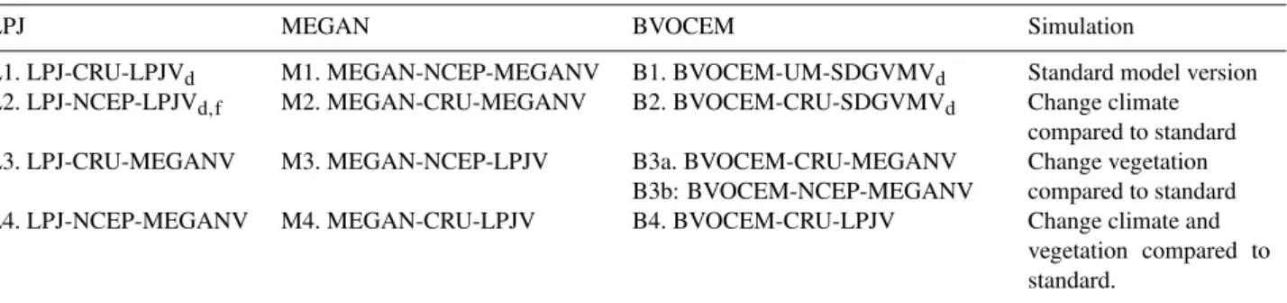
Table 1.List of simulations, described as “Model-climate-vegetation” (for example, MEGAN-CRU-LPJV is MEGAN model, run with CRU climate data and LPJ vegetation (and emission factors) and MEGAN algorithm) and MEGAN algorithm. Subscripts “d” and “f” indicate whether the DGVMs had dynamic vegetation enabled, or were driven by fixed vegetation fields.
LPJ MEGAN BVOCEM Simulation
L1. LPJ-CRU-LPJVd M1. MEGAN-NCEP-MEGANV B1. BVOCEM-UM-SDGVMVd Standard model version L2. LPJ-NCEP-LPJVd,f M2. MEGAN-CRU-MEGANV B2. BVOCEM-CRU-SDGVMVd Change climate
compared to standard L3. LPJ-CRU-MEGANV M3. MEGAN-NCEP-LPJV B3a. BVOCEM-CRU-MEGANV
B3b: BVOCEM-NCEP-MEGANV
Change vegetation compared to standard L4. LPJ-NCEP-MEGANV M4. MEGAN-CRU-LPJV B4. BVOCEM-CRU-LPJV Change climate and
vegetation compared to standard.
SDGVM and LPJ-GUESS, vegetation dynamics, PFT dis-tribution composition, and isoprene emissions are linked be-cause each of these processes respond dynamically to cli-mate. For LPJ-GUESS, experiments 2 to 4 either included prescribing vegetation cover from MODIS/MEGAN, or run-ning with NCEP climate but keeping PFT distribution fixed from the CRU standard runs. This required the use of a version of LPJ-GUESS with its standard fast-exchange pro-cesses (photosynthesis, BVOC) enabled but with applying prescribed vegetation characteristics and soil, as well as adopting the MEGAN vegetation classes for use in LPJ-GUESS (Table A1). Since isoprene emissions are directly coupled to the model’s carbon cycle simulations, parame-ters for the photosynthesis calculations were adopted for the MEGAN vegetation, primarily by applying the photosynthe-sis temperature limits from LPJ-GUESS’s equivalent PFTs. Additionally, the average area-based emission factors applied in MEGAN (Guenther et al., 2006) had to be converted into leaf-based values used in LPJ-GUESS, taking into account the modelled specific leaf area (SLA, m2leafkg C−1) and the
standard LAI used in MEGAN (5.0). This was based on the simple relationshipELP J/SLA·LAI(5)·0.42=EMEGAN;
0.42 is an empirical factor derived using a canopy environ-ment model and represents the ratio of leaf- to canopy-scale emission factors for a canopy with an LAI of 5. The in-verse equation was used to convert the LPJ leaf-level emis-sion factors to canopy-scale emisemis-sion factors. When running the BVOCEM with different vegetation classes, the emission factors had to be adapted to ensure consistency across the various PFTs and the units. For the experiments using either the SDGVM or the MEGAN vegetation patterns, globally-averaged emission factors from Guenther et al. (2006) were used. When using vegetation input provided by LPJ, the LPJ emission factors were converted to the appropriate unit using the equation above.
3 Results
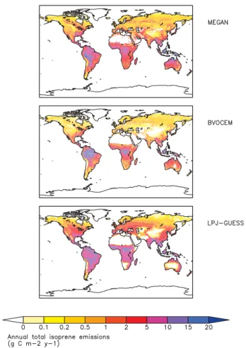
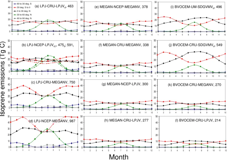
3.1 Annual totals and geographical/seasonal patterns In their standard settings (LPJ-CRU-LPJV, MEGAN-NCEP-MEGANV and BVOCEM-UM-SDGVMV) between-model variation in average global isoprene emissions was small, 378 to 496 Tg C a−1(Figs. 1, 2). Emissions for LPJ-GUESS were somewhat higher than reported in Arneth et al. (2007a; 463 vs. 410 Tg C a−1), arising from the slightly different av-eraging period, small adjustments to the way seasonally-changing emission factors were calculated, and a newly in-troduced leaf-energy balance calculation (Schurgers et al., 2011). Likewise, for the BVOCEM simulations we removed the assumed 4 % loss associated with within-canopy reac-tions in the reported 471 Tg C a−1(Lathi`ere et al., 2010). The
22-yr averaged emissions for MEGAN (378 Tg C a−1) were
lower than reported by Guenther et al. (2006) for the year 2003 (ca. 530 Tg C a−1). These, too, reflected the longer
simulation period with a slightly cooler average tempera-ture compared to 2003 alone as well as the exclusion of the soil moisture activity factor and differences in the version of NCEP temperature and solar radiation data used to drive the simulations shown here.
Fig. 1. Average annual global isoprene emissions for the period 1981–2002 from three different emission models. Averages are from the “standard” model setups in the case of LPJ-GUESS and MEGAN (see Table 1, Fig. 2, panelsa,e), and with CRU climate in the case of BVOCEM (Fig. 2, paneli).
feature that was reduced when MEGAN vegetation was ap-plied (Fig. 2k). By contrast, in MEGAN and LPJ-GUESS, magnitude and seasonal variation in the northern and south-ern tropics (0 to 30 degrees) were very similar, the average sums for−30◦ to +30◦differed by less than 20 % between the two models. All three models simulate maximum emis-sions from the northern temperate zones (30 to 60◦N) dur-ing the Northern Hemisphere summer months to be equal to emissions from either the northern or southern tropical re-gions.
3.2 Effects of varying climate input
In MEGAN and BVOCEM, changing climate affects emis-sions directly via the temperature- and light-driven emission algorithms, in the case of LPJ-GUESS the effects operate mainly via the temperature and light effects on electron trans-port rates, and the difference between the temperature opti-mum of electron transport and isoprene production. As seen
in Fig. 2, in the two DGVMs, changing climate inputs also affected calculated emissions indirectly, by altering the dis-tribution of PFTs, total leaf area and the seasonality of leaf growth (subscripts “d” in Fig. 2b, j). With dynamic vege-tation enabled, applying a different climate changed annual emissions by 3 % (LPG-GUESS; CRU to NCEP) and 10 % (BVOCEM, UM to CRU).
When run with non-standard climate but unchanged vege-tation as compared to standard runs, emissions increased no-tably in LPJ-GUESS (Fig. 2a, b) and decreased in MEGAN (Fig. 2e, f). The relative response when swapping NCEP and CRU in MEGAN and LPJ-GUESS, respectively, yielded an increase of close to 30 % in LPJ-GUESS and a decrease by a little more than 10 % in MEGAN. In both cases, apply-ing the CRU climate resulted in lower emissions compared to runs that applied NCEP climate. By contrast, a simula-tion with BVOCEM and fixed vegetasimula-tion (from MEGAN) yielded emissions higher by approximately 10 % in the CRU compared to the NCEP simulation (269 vs. 244 Tg C a−1; not shown).
Regionally, differences caused by change in climate in-put were even larger than indicated by the global sums, and more varied. Figure 3 shows the direct effects of differ-ing climate datasets only (i.e. usdiffer-ing fixed vegetation in all cases), BVOCEM exhibited uniformly higher rates of emis-sions for the CRU simulations compared to NCEP in large parts of the tropics, especially the rainforest regions, and slightly lower rates in savannas and some parts of the tem-perate forest regions. For LPJ-GUESS and MEGAN, emis-sions using NCEP versus CRU climate tended to be higher in a large part of the Northern Hemisphere temperate and bo-real biome. Emissions were also enhanced in some parts of the tropical areas, but in other tropical regions this pattern was reversed especially in case of MEGAN. In LPJ-GUESS, lower emissions in the NCEP case were, for instance, calcu-lated in northeastern and eastern South America, and parts of tropical Africa.
3.3 Effects of a change in vegetation
Alternating between the standard and an alternate vegeta-tion dataset yielded substantially higher emissions in LPJ-GUESS (Fig. 2, panel c) and lower emissions in MEGAN (panel g). For BVOCEM, a change from MEGAN to LPJ vegetation reduced emissions, but to a much smaller degree compared to the other two models (panels k and l in Fig. 2). In the case of LPJ-GUESS, the change in vegetation led to a more pronounced seasonality in emissions in tropical regions of the Southern Hemisphere, whereas in MEGAN, this sea-sonality was substantially dampened compared to the stan-dard model setup (panels e, g).
0 10 20 30 40 50
1 2 3 4 5 6 7 8 9 10 11 12
0 10 20 30 40 50
1 2 3 4 5 6 7 8 9 10 11 12
0 10 20 30 40 50
1 2 3 4 5 6 7 8 9 10 11 12
Month
Is
oprene emissions
(Tg
C
)
(c) LPJ-CRU-MEGANV, 750
(l) BVOCEM-CRU-LPJV, 214 (h) MEGAN-CRU-LPJV, 277
0 10 20 30 40 50
1 2 3 4 5 6 7 8 9 10 11 12
(d) LPJ-NCEP-MEGANV, 987
0 10 20 30 40 50
1 2 3 4 5 6 7 8 9 10 11 12
(k) BVOCEM-CRU-MEGANV, 270
0 10 20 30 40 50
1 2 3 4 5 6 7 8 9 10 11 12
(i) BVOCEM-UM-SDGVMVd, 496
0 10 20 30 40 50
1 2 3 4 5 6 7 8 9 10 11 12
(j) BVOCEM-CRU-SDGVMVd, 549
0 10 20 30 40 50
1 2 3 4 5 6 7 8 9 10 11 12
(b) LPJ-NCEP-LPJVd,f, 475d; 591f
0 10 20 30 40 50
1 2 3 4 5 6 7 8 9 10 11 12 0 10 20 30 40 50
1 2 3 4 5 6 7 8 9 10 11 12
(f) MEGAN-CRU-MEGANV, 338
(g) MEGAN-NCEP-LPJV, 300
0 10 20 30 40 50
1 2 3 4 5 6 7 8 9 10 11 12 60 to 30 deg. S
30 deg. S to 0 0 to 30 deg. N 30 to 60 deg. N 60 to 90 deg. N
0 10 20 30 40 50
1 2 3 4 5 6 7 8 9 10 11 12
(e) MEGAN-NCEP-MEGANV, 378
0 10 20 30 40 50
1 2 3 4 5 6 7 8 9 10 11 12
(e) MEGAN-NCEP-MEGANV, 378
(a) LPJ-CRU-LPJVd, 463
Fig. 2. Seasonal isoprene emissions from the different model experiments, separated by latitudinal bands (deg.: degrees). The naming convention for each simulation was “Model-climate-vegetation” (see Table 1). Panels(a),(e)and(i)are equivalent to the models published and evaluated standard settings (e.g., Arneth et al., 2007a, Guenther et al., 2006, Lathi`ere et al., 2010). Shown are averages for the period 1981–2002, except for panel(i)as the UM climate was only available for one year. Numbers in the top right corner of each panel are annual sums, in Tg C a−1. In panels(a, b)and(i,j), For the two DGVMs, subscribed “d” or “f” indicates whether the dynamic vegetation core in the model responds to the climate in the given simulation (dash-dotted line in panel(b)), or whether vegetation prescribed from the standard run was used (straight line in panel(b)).
pattern when the simulation results are plotted in their geo-spatial and temporal distribution. Only few responses were uniform in all three models when switching from MEGAN to LPJ vegetation. Simulations with MEGAN vegetation ap-pear to generally yield higher emissions in large parts of Aus-tralia, southern Africa, tropical rain forest regions and, dur-ing the Northern Hemisphere summer months, large parts of the boreal biome. In contrast, lower emissions are simulated from the South American savanna (cerrado) regions and parts of the African savannas, and in LPJ-GUESS and BVOCEM, temperate regions in Europe, Asia and the US. For most other regions the model response was varied with no obvious simi-larities with respect to the direction of the change introduced by vegetation.
3.4 Combination of effects
Fig. 3.Difference in isoprene emissions (mg C m−2month−1)for simulations performed with NCEP climate minus simulations with CRU climate (top: M1–M2; middle: B3b-B3a; bottom: L2–L1; see Table 1). In the case of the dynamic vegetation models, the differences shown are those with fixed vegetation (L2: LPJVf); and in case of BVOCEM, MEGAN vegetation was applied. Panels show monthly averages over three-month periods December to February (DJF); March to May (MAM); June to August (JJA); September to November (SON).
tropics when using LPJ together with MEGAN vegetation as well as NCEP climate. For BVOCEM-CRU runs, apply-ing fixed vegetation greatly dampened the seasonality both in southern and northern tropics compared to runs where vege-tation responded dynamically to seasonal climate.
3.5 Interannual variability
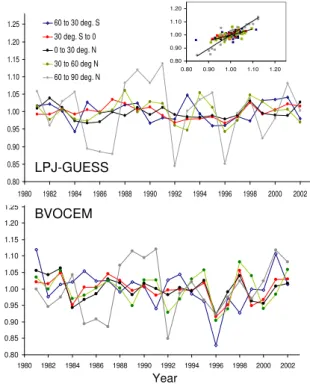
In their dynamic vegetation configuration, interannual vari-ability of normalised and detrended annual isoprene emis-sions was found for both LPJ-GUESS and BVOCEM to be larger in the high northern latitudes than in any other of the latitude bands, varying by up to 15 % (Fig. 5). In the other regions, maximum between-year variability in emission rates was around 5 % in LPJ-GUESS, and around 10 % in BVO-CEM. A clear linear relationship between the annual iso-prene emission rate output of the two models emerged, but
with a distinctly different slope for the latitudinal band 60– 90◦N (1.06) and the other regions (c. 0.4, Fig. 5, inset). The close relationship between the two models, occurring despite different isoprene algorithms, emission capacities and simu-lated vegetation patterns suggests on a decadal perspective a mostly climate-driven variability in isoprene emissions from one year to the next, since the models were driven by the same climate in these experiments (CRU).
Fig. 4. Difference in isoprene emissions (mg C m−2month−1)for simulations performed with MEGAN vegetation minus LPJ-GUESS vegetation. Panels show monthly averages over three-month periods, the same as those in Fig. 3 (top: M1–M3; middle: B3a–B4; bottom: L3–L1, see Table 1).
where isoprene production is closely linked to photosyn-thesis, interannual variability in gross primary productivity (GPP) was somewhat larger (standard deviation around the mean was up to∼10 %, for the normalised and detrended data) than for isoprene, and with the exception of the north-ernmost band, no common patterns emerged between vari-ability in isoprene and that in GPP. For BVOCEM, where emissions scale directly with leaf area index, rather than with primary productivity, interannual variability in LAI of the chief emitting PFTs was of the same magnitude than for iso-prene, but here, too, a relationship between variation in LAI and that in isoprene was only notable for the 60 to 90◦N band, as well as (but weaker) for the regions between 30 and 60◦N (not shown).
4 Discussion
Comparing the three models in their published standard ver-sions confirms previous global simulations in that the global isoprene source is clearly dominated by the tropical regions (see Guenther et al., 1995; Arneth et al., 2008a, and refer-ences therein). The standard versions monthly emission rates varied between ca. 10 and 25 Tg C in the two bands bound by 30 degrees latitude north and south of the equator. The three models also simulated seasonal maxima in northern temper-ate regions that were of the same magnitude as in the trop-ics. Annual global emission totals were within the range of previously published studies, with MEGAN being somewhat lower than what is typically found in bottom-up global mod-els (Arneth et al., 2008a).
0.80 0.85 0.90 0.95 1.00 1.05 1.10 1.15 1.20 1.25 1.30
1980 1982 1984 1986 1988 1990 1992 1994 1996 1998 2000 2002
Normalised
isoprene emissions (detrended)
Year
BVOCEM
0.80 0.85 0.90 0.95 1.00 1.05 1.10 1.15 1.20 1.25
1980 1982 1984 1986 1988 1990 1992 1994 1996 1998 2000 2002
60 to 30 deg. S
30 deg. S to 0 0 to 30 deg. N
30 to 60 deg N 60 to 90 deg. N
LPJ-GUESS
0.80 0.90 1.00 1.10 1.20
0.80 0.90 1.00 1.10 1.20
Fig. 5. Annual total emissions from LPJ-GUESS (top panel) and BVOCEM (bottom panel), separated by latitudinal band, over the 22-yr simulation period. Simulations were performed by apply-ing the CRU climate and with dynamic vegetation features enabled. CO2concentration affected vegetation productivity, but the direct effects of CO2on isoprene production were disabled. Data were normalised to unity by the average emission rate over the simula-tion period, and a linear trend was removed. The inset shows the correlation between the two models, with a separate regression for the northernmost latitudinal band (60–90◦N, grey).
tropical gridcell located in the Amazon has also been found in a simulation by Levis et al. (2003), who simulated the sea-sonal emission maximum around February–March and a sec-ond, smaller peak around July-August. Emission minima oc-curred around months 6 and 11. Satellite-retrieved formalde-hyde (HCHO) concentrations indicated minima in HCHO concentrations above the Amazon from April to June, corre-sponding with the transition period between the wet and the dry season (Barkley et al., 2008, 2009). As HCHO is a prin-cipal atmospheric isoprene oxidation product, these patterns have been interpreted as a seasonal isoprene emission low, arising from a lag between substantial new leaf area growth (which takes place during that period of the year and con-tinues well into the dry season; Huete et al., 2006; Myneni et al., 2007) and the delayed onset of isoprene emission in newly-developed leaves. However, in warm growth environ-ments, the period between onset of photosynthesis and iso-prene emissions in newly-emerging foliage has been found to be short (Kuhn et al., 2004; Wiberley et al., 2005), lags on the order of weeks may thus be difficult to fully reconcile with the process of leaf growth alone.
0 0.5 1 1.5 2 2.5 3 3.5
0 200 400 600 800 1000 1200 1400
Buckley 2001 Centritto et al. 2004 Li et al. 2009 Monson et al. 1989, 2007 Possell et al. 2005 Rosenstiel et al., 2003 Scholefield et al. 2004 Sharkey et al. 1991 Wilkinson et al. 2009 Possell & Hewitt 2010 Arneth et al., (ci/ci_370) Possell_fit Wilkinson_fit
Leaf isoprene emissions (normalised)
Growth CO2concentration (ppm)
Fig. 6. Leaf-level response of isoprene emissions to varying CO2 growth environment. Symbols represent observations from a num-ber of studies and plant species, and are normalised to be unity at growth CO2concentration (Ca) ofc370 ppm. Data shown are
only from emission measurements that were undertaken at the CO2 growth concentration. The lines represent three different algorithms that are currently being applied to represent the observed response in global models: (i) the empirical function proposed by Possell et al. (2005), used e.g., for BVOCEM in (Lathi`ere et al., 2010); (ii) a function representing the ratio of change in (non water-stressed) leaf-internal CO2concentration (Ci) toCiat 370 ppm, used e.g., for
LPJ-GUESS in (Ci/Ci−370; Arneth et al., 2007a), which can be
in-terpreted as reflecting the varying leaf-internal competition for CO2 (Rosenstiel et al., 2004) – this line is by chance nearly identical to the empirical function in (i); (iii) a “Hill”-type function proposed by Wilkinson et al. (2009), withCi estimated as 0.7×Ca in
anal-ogy to the same assumption applied in LPJ-GUESS (Arneth et al., 2007b). Approach (iii) has been adopted for MEGAN e.g., in Heald et al. (2009). The Figure is adapted from Young et al. (2009), and updated with latest published observations.
In Fig. 2, latitudinal and longitudinal averaging blurs some features that may be typical for the Amazon with that of other tropical regions, and the simulated patterns thus do not show clearly-defined emission maxima during the dry season in the Southern Hemisphere tropics (Barkley et al., 2009). Still, the calculated seasonal variation appears reasonable when com-pared to the limited number of canopy-scale measurements from the tropical regions which have demonstrated similar or even much larger differences between emission minima and maxima throughout the year (Karl et al., 2004, 2007; Muller et al., 2008), and is, in the model simulations, related to com-bination of variation in leaf area index, incident radiation and air temperature.
temperature difference of approximately 0.8 K averaged over our simulation period, especially in the tropical regions. This gives rise to expectations that emissions would decrease in experiments that move from CRU to NCEP climate, and vice versa. But this response was only observed in the BVOCEM (using fixed MEGAN vegetation) simulation.
The NCEP climate product tends to be wetter in some re-gions when compared with CRU. In LPJ-GUESS, increased precipitation in dry regions would stimulate rates of photo-synthesis (Schaphoff et al., 2006) and hence isoprene produc-tion, which could contribute to enhanced emissions. When vegetation responds dynamically to the NCEP climate, an additional influence is via changes in the PFT distribution, which in the tropical areas was shifted towards the evergreen type in the NCEP simulations, with lower emission capaci-ties compared to raingreen vegetation (not shown). Such a vegetation shift compensates for the climate effects to some degree, since the evergreen PFT has a lower emission capac-ity compared to tropical raingreen vegetation (Arneth et al., 2007a).
Finally, a third confounding factor could be radiation lev-els. In the CRU product, radiation is given as percent cloudi-ness, which can be transformed into incident solar radiation as a function of solar angle, shortwave albedo and clear sky atmospheric transmissivity (Monteith and Unsworth, 1990). The resulting insolation was lower than in the NCEP product (not shown) and is probably a chief driver behind the increase of emissions in LPJ-GUESS + NCEP, as well as the lower an-nual emissions in MEGAN+CRU compared to their respec-tive standard cases. Previous calculations using the MEGAN standard case but with CRU climate also led to reductions of approximately similar magnitude than here (−11 %; Guen-ther et al., 2006). This smaller sensitivity was caused by taking a different approach to convert CRU cloud cover into irradiance levels, based on the BEIS inventory-model algo-rithms (Pierce et al. 1998), as well as from different time av-eraging for the comparison which was based on a single year (2003). Overall, the multifaceted interactions between vary-ing temperatures, radiation and precipitation highlight why a simple extrapolation to expected emission changes under fu-ture or past climate changes, based on the models’ responses for present-day, would be problematic.
LPJ-GUESS tends to simulate lower LAI in most parts of Australia and southern Africa compared to the MODIS prod-uct used in MEGAN (see e.g., Sitch et al., 2003; Guenther et al., 2006), which can explain the model-to-model differ-ences in these regions seen in Fig. 4. Moreover, changing from MEGAN vegetation to LPJ vegetation also meant a change from accounting for crops to potential natural veg-etation, hence the lower emission rates in parts of Europe, Asia and the U.S. calculated by LPJ GUESS and BVOCEM when applying MEGAN vegetation. Lathi`ere et al. (2010) found global crop area to cause a 15 % reduction of emis-sions in late 20th century isoprene emisemis-sions compared to a simulation with potential natural vegetation, and by ca. 30
to 40 % in northern America and Europe, respectively. In an LPJ-GUESS simulation for Europe, emissions after account-ing for crop area were reduced by more than a factor of three (Arneth et al., 2008b). At the same time, changes in PFT dis-tribution and emission factors also play an important role in the interpretation of the observed between-model responses to variable vegetation. For instance, MEGAN assigns large parts of Australia to be covered by shrubs with high emission potentials (Guenther et al., 2006), while LPJ-GUESS simu-lates these areas to be dominated by grassland rather than woody vegetation (Sitch et al., 2003) that has a much lower emission potential.
The boreal forest regions, where all models respond with a decrease in emissions when applying LPJ vegetation com-pared to MEGAN vegetation have a large component of fine-leaf evergreen and shrub vegetation in MEGAN, and a mix of broadleaf deciduous and evergreen conifers as well as (in Eastern Siberia) deciduous conifers in LPJ-GUESS. The de-crease is hence mainly to be interpreted in view of the emis-sion capacities since, after converemis-sion to common units, only the boreal broadleaf summergreen PFTs had higher emis-sion factors compared to shrubs and fineleaf PFTs. Pfister et al. (2008) examined the sensitivity of MEGAN to land cover inputs using three different sets of satellite-derived LAI and PFT datasets and reported a factor of 2 or more difference on global to regional scales. This analysis highlights the uncer-tainties in land-cover estimates, affecting emission capacities as well as also canopy structural properties, and continued improvements in these data will eventually lead to more ac-curate emission estimates.
Interannual variability in emission rates was found to be small, except for the northernmost latitudinal band, where emissions are very low in absolute terms. Although some of the anomalies (i.e., the low rates in 1992) corresponded to climate fluctuations (i.e., cool summer temperatures follow-ing the Mount Pinatubo eruption, and subsequent effects on emissions; (Lucht et al., 2002; Telford et al., 2010)) the vari-ation in precipitvari-ation and temperature for regions between 60 to 90◦N were not substantially larger than in the other lati-tude bands, and the magnilati-tude of the interannual variation hence cannot be directly attributed to larger climate fluctua-tions in that region. Considering both regional and interan-nual variability, fluctuations of typically not more than 5 and (exceptional) 10 % around the mean have also been found for simulated isoprene emissions when applying the DGVM ORCHIDEE for the period 1983 to 1995 (Lathi`ere et al., 2006).
initially seem counterintuitive, as for instance warm weather conditions that foster isoprene emissions should also enhance GPP and LAI – by lengthening growing season or by be-ing closer to the temperature-optimum for photosynthesis. But warm temperatures can also coincide with soil-water deficit, thereby reducing GPP and LAI, or, especially in trop-ical and subtroptrop-ical regions, exceeding optimal photosyn-thetic temperatures. Moreover, computing annual averages across latitudinal bands can hide regionally-variable patterns that might otherwise reveal how weather and emissions co-vary (Lathi`ere et al., 2006). Better understanding of how the various environmental factors and the associated vegetation growth responses interact would require flux sites where iso-prene fluxes are measured over a number of years alongside ecosystem-atmosphere CO2exchange measurements, but we
are only aware of one such data set (Pressley et al., 2005) with four years of measurements. Interannual variability re-ported at this site, an aspen- and red oak-dominated hard-wood forest, was less than 10 %.
4.1 Short-term vs. long-term emission patterns
The strong temperature-sensitivity of leaf emissions and an-ticipated warmer temperatures in a high-CO2 world have
been the chief argument for assuming a greatly enhanced fu-ture isoprene source in simulations of fufu-ture trace gas com-position (e.g., Sanderson et al., 2003; Hauglustaine et al., 2005; Young et al., 2009). Increased atmospheric CO2
lev-els also enhance rates of leaf photosynthesis. It is expected that this CO2fertilisation will sustain an enhanced vegetation
productivity, even though acclimation processes on leaf- and canopy-scales, as well as nutrient or water limitations, may reduce the overall vegetation growth effects to below what is extrapolated from short-term leaf-level observations alone (K¨orner, 2006; Finzi et al., 2007; Hickler et al., 2008). The concomitant LAI increase would foster heightened isoprene emissions compared to present-day in addition to a direct temperature effect. However, an increasing number of stud-ies have also shown a direct CO2- effect on isoprene
emis-sions, such that leaf emissions decline at above-ambient CO2
levels, possibly due to leaf-internal competition for some iso-prene precursor substances (Rosenstiel et al., 2003; Possell et al., 2005; Wilkinson et al., 2009). Here, too, some com-pensatory effects can be detected, such that the response to varying CO2differs depending on whether leaf area or mass
is used as the reference, or whether leaf or whole plant emis-sions are being considered (Possell et al., 2005; Possell and Hewitt, 2010).
Global isoprene models are beginning to include a direct CO2-leaf emission response, adopting different algorithms
that are summarised in Fig. 6 (Arneth et al., 2007a; Heald et al., 2009; Lathi`ere et al., 2010; Pacifico et al., 2011). In fu-ture scenarios, accounting for CO2inhibition has been shown
to decrease emissions notably (several 10s of a percent com-pared to present-day) in simulations that kept vegetation
fixed. The overall reduction depends on both the choice of the CO2scenario and the magnitude of temperature increase
(Heald et al., 2009; Arneth et al., 2007a). Including the ad-ditional effects of a dynamic vegetation response combines effects of altered productivity as well as changing vegetation PFT mixtures on global emissions, which makes between-study comparisons difficult. After accounting for the addi-tional direct CO2 inhibition effect, the projected emission
increase in response to warmer temperatures and enhanced leaf area was either reduced (applying MEGAN in the Com-munity Land Model, and for the IPCC SRES scenario A1B; Heald et al., 2009), or emissions were close to present-day rates (range of SRES and climate models; Arneth et al., 2007a). In these two studies, global average LAI was mod-elled to increase more than three-fold (Heald et al., 2009), vs. by between 2 and 27 % (Arneth et al., 2007a). Though LAI is not the sole factor explaining the diverging between-model responses to climate and CO2 change, these differences in
LAI highlight the equal importance of developing robust pro-jections of vegetation response to environmental changes in addition to improving process-based leaf-level isoprene al-gorithms. Assessments of future levels of air pollution and climate change respond sensitively to variation in future iso-prene emissions (Sanderson et al., 2003; Hauglustaine et al., 2005; Young et al., 2009). A full and internally-consistent accounting of the suite of environmental and direct (i.e., land use/land cover change; Arneth et al., 2008b; Lathi`ere et al., 2006, 2010) anthropogenic drivers that affect biogenic emis-sions, together with an accurate understanding of the mani-fold interactions and impacts caused by each of these drivers hence is necessary.
5 Conclusion
Appendix A
Table A1.Use of plant functional types and isoprene emission factors for simulations in this study (dm: dry matter).
LPJ-GUESS PFTs
Abbrev. Emission factor (µg C g−1 leafdmh−1)
Emission factor (mg C m−2 ground h−1)
for the BVOCEM running with LPJ vegetation
MEGAN PFTs
Abbrev. LPJ assigned BVOCEM– SDGVM PFTs
Emission factor (mg C m−2 ground h−1)
for the BVO-CEM running with SDGVM vegetation
1. Tropical Broadleaved Evergreen
TrBE 24.0 4.6 1. Broadleaf
trees
btr 1, 2, 4, 5 and 8 1. C3 grass 0.4
2. Tropical Broadleaved Raingreen
TrBR 45.0 4.6 2. Fineleaf
trees
ftr 3, 6 and 7 2. C4 grass 0.4
3. Temperate Needleleaved Evergreen
TeNE 16.0 3.1 3. Grass and
herbaceous
grs 9 and10 3. Evergreen broadleaf trees
11.1
4. Temperate Broadleaved Evergreen
TeBE 24.0 3.4 4. Shrubs shr Adapted from
1, 2, 4, 5 and 8
4. Evergreen Needleleaf trees
1.8
5. Temperate Broadleaved Summergreen
TeBS 45.0 4.6 5. Herbaceous
and shrubby crops
crp Adapted from 9 and 10
5. Deciduous broadleaf trees
11.1
6. Boreal Needleleaved Evergreen
BNE 8.0 1.5 6. Deciduous
needleleaf trees 0.6
7. Boreal Needleleaved Summergreen
BNS 8.0 0.8
8. Boreal Broadleaved Summergreen
BBS 45.0 4.6
9. C3 herbaceous C3 16.0 1.6 10. C4 herbaceous C4 8.0 0.82
Acknowledgements. This work was supported by a Human Frontier Science Programme grant to AA, and contributes to the EU FP7 IP PEGASOS (FP7-ENV-2010/265148). AA and GS acknowledge additional support from the Swedish Research Councils Formas (2007-331) and VR (2005-4039; 2009-4290), and from an Alexander von Humboldt Foundation Guest-Fellowship to AA at IMK-IFU. The BVOCEM development was part of the UK Natural Environment Research Council’s Quantifying and Understanding the Earth System (QUEST) Research Programme (grant NE/C001621/1).
Edited by: J. Rinne
References
Arneth, A., Miller, P. A., Scholze, M., Hickler, T., Schurg-ers, G., Smith, B., and Prentice, I. C.: CO2 inhibition of global terrestrial isoprene emissions: Potential implications for atmospheric chemistry, Geophys. Res. Lett., 34, L18813, doi:10.11029/12007GL030615, 2007a.
Arneth, A., Niinemets, U., Pressley, S., B¨ack, J., Hari, P., Karl, T., Noe, S., Prentice, I. C., Serca, D., Hickler, T., Wolf, A., and Smith, B.: Process-based estimates of terrestrial ecosys-tem isoprene emissions: incorporating the effects of a
di-rect CO2-isoprene interaction, Atmos. Chem. Phys., 7, 31–53, doi:10.5194/acp-7-31-2007, 2007b.
Arneth, A., Monson, R. K., Schurgers, G., Niinemets, U., and Palmer, P. I.: Why are estimates of global isoprene emissions so similar (and why is this not so for monoterpenes)?, At-mos. Chem. Phys., 8, 4605–4620, doi:10.5194/acp-8-4605-2008, 2008a.
Arneth, A., Schurgers, G., Hickler, T., and Miller, P. A.: Effects of species composition, land surface cover, CO2concentration and climate on isoprene emissions from European forests, Plant Biol., 10, 150–162, doi:110.1055/s-2007-965247, 2008b. Arneth, A., Sitch, S., Bondeau, A., Butterbach-Bahl, K., Foster,
P., Gedney, N., de Noblet-Ducoudre, N., Prentice, I. C., Sander-son, M., Thonicke, K., Wania, R., and Zaehle, S.: From biota to chemistry and climate: towards a comprehensive description of trace gas exchange between the biosphere and atmosphere, Bio-geosciences, 7, 121–149, doi:10.5194/bg-7-121-2010, 2010. Ashworth, K., Wild, O., and Hewitt, C. N.: Sensitivity of
iso-prene emission estimated using MEGAN to the time resolu-tion of input climate data, Atmos. Chem. Phys., 10, 1193–1201, doi:10.5194/acp-10-1193-2010, 2010.
Atkinson, R.: Atmospheric chemistry of VOCs and NOx, Atmos.
Environ., 34, 2063–2101, 2000.
Net ecosystem fluxes of isoprene over tropical South America in-ferred from GOME observations of HCHO columns, J. Geophys. Res., 113, D20304, doi:10.21029/22008jd009863, 2008. Barkley, M. P., Palmer, P. I., De Smedt, I., Karl, T., Guenther, A.,
and Van Roozendael, M.: Regulated large-scale annual shut-down of Amazonian isoprene emissions?, Geophys. Res. Lett., 36, L04803, doi:10.01029/02008GL036843, 2009.
Barkley, M. P., Palmer, P. I., Ganzeveld, L., Arneth, A., H˚agberg, D., Karl, T., Guenther, A., Paulot, F., Wennberg, P. O., Mao, J., Kurosu, T. P., Chance, K., Muller, J.-F., De Smedt, I.,Van Roozendael, M., Chen, D., Wang, Y., and Yantosca, R. M.: Can a ‘state of the art’ chemistry transport model simulate Amazonian tropospehric chemistry?, J. Geophys. Res., accepted, 2011. Beerling, D. J. and Woodward, F. I.: Vegetation and the terrestrial
carbon cycle. Modelling the first 400 Million years, Cambridge University Press, Cambridge, UK, 2001.
Buckley, P. T.: Isoprene emissions from a Florida scrub oak species grown in ambient and elevated carbon dioxide, Atm. Env., 35, 631–634, 2001.
Centritto, M., Nascetti, P., Petrilli, L., Raschi, A., and Loreto, F.: Profiles of isoprene emission and photosynthetic parameters in hybrid poplars exposed to free-air CO2enrichment, Plant Cell Environ., 27, 403–412, 2004.
Claeys, M., Graham, B., Vas, G., Wang, W., Vermeylen, R., Pashyn-ska, V., Cafmeyer, J., Guyon, P., Andreae, M. O., Artaxo, P., and Maenhaut, W.: Formation of secondary organic aerosols through photooxidation of isoprene, Science, 303, 1173–1176, 2004. Finzi, A. C., Norby, R. J., Calfapietra, C., Gallet-Budynek, A.,
Gielen, B., Holmes, W. E., Hoosbeek, M. R., Iversen, C. M., Jackson, R. B., Kubiske, M. E., Ledford, J., Liberloo, M., Oren, R., Polle, A., Pritchard, S., Zak, D. R., Schlesinger, W. H., and Ceulemans, R.: Increases in nitrogen uptake rather than nitrogen-use efficiency support higher rates of temperate forest produc-tivity under elevated CO2, Proc. Natl. Acad. Sci., 104, 14014– 14019, doi:10.1073/pnas.0706518104, 2007.
Gerten, D., Schaphoff, S., Haberlandt, U., Lucht, W., and Sitch, S.: Terrestrial vegetation and water balance - hydrological eval-uation of a dynamic global vegetation model, J. Hydrol., 286, 249–270, 2004.
Guenther, A., Monson, R. K., and Fall, R.: Isoprene and monoter-pene emission rate variability: Observations with Eucalyptus and emission rate algorithm development, J. Geophys. Res., 96, 10799–10808, 1991.
Guenther, A., Hewitt, C. N., Erickson, D., Fall, R., Geron, C., Graedel, T., Harley, P., Klinger, L., Lerdau, M., McKay, W. A., Pierce, T., Scholes, B., Steinbrecher, R., Tallamraju, R., Taylor, J., and Zimmermann, P.: A global model of natural volatile or-ganic compound emissions, J. Geophys. Res., 100, 8873–8892, 1995.
Guenther, A., Karl, T., Harley, P., Wiedinmyer, C., Palmer, P. I., and Geron, C.: Estimates of global terrestrial isoprene emissions using MEGAN (Model of Emissions of Gases and Aerosols from Nature), Atmos. Chem. Phys., 6, 3181-3210, doi:10.5194/acp-6-3181-2006, 2006.
Hansen, M., DeFries, R. S., Townshend, J. R. G., Carroll, M., Dim-iceli, C., and Sohlberg, R. A.: Global percent tree cover at a spatial resolution of 500 meters: first results of the MODIS vege-tation continuous fields algorithm, Earth Interact., 7, 1–15, 2003. Hauglustaine, D. A., Lathiere, J., Szopa, S., and Folberth,
G. A.: Future tropospheric ozone simulated with a climate-chemistry-biosphere model, Geophys. Res. Lett., 32, L24807, doi:10.1029/22005GL024031, 2005.
Heald, C. L., Wilkinson, M. J., Monson, R. K., Alo, C. A., Wang, G. L., and Guenther, A.: Response of isoprene emission to ambient CO2changes and implications for global budgets, Glob. Change Biol., 15, 1127–1140, doi:10.1111/j.1365-2486.2008.01802.x, 2009.
Hickler, T., Smith, B., Prentice, I. C., Mj¨ofors, K., Miller, P., Arneth, A., and Sykes, M.: CO2fertilization in temper-ate FACE experiments not representative of boreal and tropi-cal forests, Global Change Biol., 14, 1–12, doi:10.1111/j.1365-2486.2008.01598.x, 2008.
Huete, A. R., Didan, K., Shimabukuro, Y. E., Ratana, P., Saleska, S. R., Hutyra, L. R., Yang, W., Nemani, R. R., and Myneni, R.: Amazon rainforests green-up with sunlight in dry season, Geo-phys. Res. Lett., 33, L06405, doi:10.1029/2005gl025583, 2006. Karl, T., Potosnak, M., Guenther, A., Clark, D., Walker, J.,
Her-rick, J. D., and Geron, C.: Exchange processes of volatile organic compounds above a tropical rain forest: Implications for model-ing tropospheric chemistry above dense vegetation, J. Geophys. Res., 109, D18306, doi:10.11029/12004JD004738, 2004. Karl, T. G., Christian, T. J., Yokelson, R. J., Artaxo, P., Hao,
W. M., and Guenther, A.: The tropical forest and fire emis-sions experiment: method evaluation of volatile organic com-pound emissions measured by PTR-MS, FTIR, and GC from tropical biomass burning, Atmos. Chem. Phys., 7, 5883–5897, doi:10.5194/acp-7-5883-2007, 2007.
Kiendler-Scharr, A., Wildt, J., Maso, M. D., Hohaus, T., Kleist, E., Mentel, T. F., Tillmann, R., Uerlings, R., Schurr, U., and Wahner, A.: New particle formation in forests inhibited by isoprene emis-sions, Nature, 461, 381–384, doi:10.1038/nature08292, 2009. Kistler, R., Kalnay, E., Collins, W., Saha, S., White, G., Woollen,
J., Chelliah, M., Ebisuzaki, W., Kanamitsu, M., Kousky, V., van den Dool, H., Jenne, R., and Fiorino, M.: The NCEP-NCAR 50-year reanalysis: Monthly means CD-ROM and documentation, Bulletin of the American Meteorological Society, 82, 247–267, 2001.
K¨orner, C.: Plant CO2responses: an issue of definition, time and resource supply, New Phytol., 172, 393–411, 2006.
Kuhn, U., Rottenberger, S., Biesenthal, T., Wolf, A., Schebeske, G., Ciccioli, P., and Kesselmeier, J.: Strong correlation between isoprene emission and gross photosynthetic capacity during leaf phenology of the tropical tree speciesHymenaea courbarilwith fundamental changes in volatile organic compounds emission composition during early leaf development, Plant, Cell, Environ., 27, 1469–1485, 2004.
Lathi`ere, J., Hauglustaine, D. A., Friend, A., De Noblet-Ducoudr´e, N., Viovy, N., and Folberth, G.: Impact of climate variability and land use changes on global biogenic volatile organic compound emissions, Atmos. Chem. Phys., 6, 2129–2146, doi:10.5194/acp-6-2129-2006, 2006.
Lathi`ere, J., Hewitt, C. N., and Beerling, D. J.: Sensitiv-ity of isoprene emissions from the terrestrial biosphere to 20th century changes in atmospheric CO2 concentration, cli-mate, and land use, Glob. Biogeochem. Cycl., 24, GB1004, doi:10.1029/2009GB003548, 2010.
Taraborrelli, D., and Williams, J.: Atmospheric oxidation capac-ity sustained by a tropical forest, Nature, 452, 737–740, 2008. Levis, S., Wiedinmyer, C., Bonan, G. B., and Guenther, A.:
Simu-lating biogenic volatile organic compound emissions in the Com-munity Climate System Model, J. Geophys. Res., 108, 4659, doi:10.1029/2002JD003203, 2003.
Li, D. W., Chen, Y., Shi, Y., He, X. Y., and Chen, X.: Impact of elevated CO2and O3concentrations on biogenic volatile or-ganic compounds emissions fromGinkgo biloba, Bull. Environ. Contam. Toxicol., 82, 473–477, doi:10.1007/s00128-008-9590-7, 2009.
Lichtenthaler, H. K.: The 1-deoxy-D-xylulose-5-phosphate path-way of isoprenoid biosynthesis in plants, Ann. Rev. Plant Phys. Plant Mol. Biol., 50, 47–65, 1999.
Lucht, W., Prentice, I. C., Myneni, R. B., Sitch, S., Friedlingstein, P., Cramer, W., Bousquet, P., Buermann, W., and Smith, B.: Cli-matic control of the high-latitude vegetation greening trend and Pinatubo effect, Science, 296, 1687–1689, 2002.
Mitchell, T. D. and Jones, P. D.: An improved method of construct-ing a database of monthly climate observations and associated high-resolution grids, Int. J. Climatol., 25, 693–712, 2005. Monson, R. K. and Fall, R.: Isoprene emission from aspen leaves:
Influence of environment and relation to photosynthesis and pho-torespiration, Plant Phys., 90, 267–274, 1989.
Monson, R. K.,Trahan, N., Rosenstiel, T. N.,Veres, P., Moore, D., Wilkinson, M., Norby, R. J.,Volder, A.,Tjoelker, M. G.,Briske, D. D., Karnosky, D. F., and Fall, R.: Isoprene emission from terrestrial ecosystems in response to global change: minding the gap between models and observations, Phil. Trans. Roy. Soc. A, 365, 1677–1695, 2007.
Monteith, J. L. and Unsworth, M.: Principles of Environmental Physics, 2nd ed., Arnold, London, 1990.
Morales, P., Sykes, M. T., Prentice, I. C., Smith, P., Smith, B., Bug-mann, H., Zierl, B., Friedlingstein, P., Viovy, N., Sabate, S., Sanchez, A., Pla, E., Gracia, C. A., Sitch, S., Arneth, A., and Ogee, J.: Comparing and evaluating process-based ecosystem model predictions of carbon and water fluxes in major European forest biomes, Global Change Biol., 11, 2211–2233, 2005. Muller, J. F., Stavrakou, T., Wallens, S., De Smedt, I., Van
Roozen-dael, M., Potosnak, M. J., Rinne, J., Munger, B., Goldstein, A., and Guenther, A. B.: Global isoprene emissions estimated using MEGAN, ECMWF analyses and a detailed canopy environment model, Atmos. Chem. Phys., 8, 1329–1341, doi:10.5194/acp-8-1329-2008, 2008.
Myneni, R. B., Yang, W. Z., Nemani, R. R., Huete, A. R., Dick-inson, R. E., Knyazikhin, Y., Didan, K., Fu, R., Juarez, R. I. N., Saatchi, S. S., Hashimoto, H., Ichii, K., Shabanov, N. V., Tan, B., Ratana, P., Privette, J. L., Morisette, J. T., Vermote, E. F., Roy, D. P., Wolfe, R. E., Friedl, M. A., Running, S. W., Votava, P., El-Saleous, N., Devadiga, S., Su, Y., and Sa-lomonson, V. V.: Large seasonal swings in leaf area of Ama-zon rainforests, Proc. Natl. Acad. Sci. USA, 104, 4820–4823, doi:10.1073/pnas.0611338104, 2007.
Naik, V., Delire, C., and Wuebbles, D. J.: Sensitivity of global biogenic isoprenoid emissions to climate variabil-ity and atmospheric CO2, J. Geophys. Res., 109, D06301, doi:10.01029/02003JD004236, 2004.
Niinemets, U., Tenhunen, J. D., Harley, P. C., and Steinbrecher, R.: A model of isoprene emission based on energetic requirements
for isoprene synthesis and leaf photosynthetic properties for Liq-uidambarand Quercus, Plant, Cell, Environ., 22, 1319–1335, 1999.
Niinemets, ¨U., Arneth, A., Kuhn, U., Monson, R. K., Pe˜nuelas, J., and Staudt, M.: The emission factor of volatile iso-prenoids: stress, acclimation, and developmental responses, Biogeosciences, 7, 2203–2223, doi:10.5194/bg-7-2203-2010, 2010a.
Niinemets, ¨U., Monson, R. K., Arneth, A., Ciccioli, P., Kesselmeier, J., Kuhn, U., Noe, S. M., Penuelas, J., and Staudt, M.: The emission factor of volatile isoprenoids: caveats, model algo-rithms, response shapes and scaling, Biogeosciences, 7, 1809-1832, doi:10.5194/bg-7-1809-2010, 2010b.
Pacifico, F., Harrison, S. P., Jones, C. D., Arneth, A., Sitch, S., Weedon, G. P., Barkley, M. P., Palmer, P. I., Serc¸a, D., Poto-snak, M., Fu, T. M., Goldstein, A., Bai, J., and Schurgers, G.: Evaluation of a photosynthesis-based biogenic isoprene emission scheme in JULES and simulation of isoprene emissions under modern climate conditions, Atmos. Chem. Phys., 11, 4371-4389, doi:10.5194/acp-11-4371-2011, 2011.
Palmer, P. I., Abbot, D. S., Fu, T. M., Jacob, D. J., Chance, K., Kurosu, T. P., Guenther, A., Wiedinmyer, C., Stanton, J. C., Pilling, M. J., Pressley, S. N., Lamb, B., and Sumner, A. L.: Quantifying the seasonal and interannual variability of North American isoprene emissions using satellite observations of the formaldehyde column, J. Geophys. Res., 111, D12315, doi:10.11029/12005JD006689, 2006.
Pfister, G. G., Emmons, L. K., Hess, P. G., Lamarque, J. F., Orland o, J. J., Walters, S., Guenther, A., Palmer, P. I., and Lawrence, P. J.: Contribution of isoprene to chemical budgets: A model tracer study with the NCAR CTM MOZART-4, J. Geophys. Res., 113, D05308, doi:10.01029/02007JD008948, 2008.
Poisson, N., Kanakidou, M., and Crutzen, P. J.: Im-pact of non-methane hydrocarbons on tropospheric chem-istry and the oxidizing power of the global troposphere: 3-dimensional modelling results, J. Atmos. Chem., 36, 157–203, doi:10.1023/A:1006300616544, 2000.
Possell, M., Hewitt, N. C., and Beerling, D. J.: The effects of glacial atmospheric CO2concentrations and climate on isoprene emis-sions by vascular plants, Global Change Biol., 11, 60–69, 2005. Possell, M. and Hewitt, C. N.: Isoprene emissions from plants are
mediated by atmospheric CO2 concentrations, Global Change Biol., doi:10.1111/j.1365-2486.2010.02306.x, 2010.
Prather, M., Ehhalt, D., Dentener, F. J., Derwent, R., Dlugokencky, E. J., Holland , E., Isaksen, I., Katima, J., Kirchhoff, V., Mat-son, P., Midgley, P., M., W., and al., e.: Atmospheric chemistry and greenhouse gases, in: Climate Change 2001. The Scientific Basis. Contribution of Working Group I to the Third Assess-ment Report of the IntergovernAssess-mental Panel on Climate Change, edited by: Houghton, J. T., Ding, Y., Griggs, D. J., Noguer, M., van der Linden, P. J., Dai, X., Maskell, K., and Johnson, C. A., University Press, Cambridge, 238–287, 2001.
Pressley, S., Lamb, B., Westberg, H., Flaherty, J., Chen, J., and Vogel, C.: Long-term isoprene flux measurements above a northern hardwood forest, J. Geophys. Res., 110, D07301, doi:07310.01029/02004JD005523, 2005.
259, doi:210.1038/nature01312, 2003.
Rosenstiel, T. N., Ebbets, A. L., Khatri, W. C., Fall, R., and Mon-son, R. K.: Induction of Poplar leaf nitrate reductase: A test of extrachloroplastic control of isoprene emission rate, Plant Biol., 6, 12–21, 2004.
Sanderson, M. G., Jones, C. D., Collins, W. J., Johnson, C. E., and Derwent, R. G.: Effect of climate change on isoprene emis-sions and surface ozone levels, Geophys. Res. Lett., 30, 1936, doi:1910.1029/2003GL017642, 2003.
Schaphoff, S., Lucht, W., Gerten, D., Sitch, S., Cramer, W., and Prentice, I. C.: Terrestrial biosphere carbon storage under alter-native climate projections, Clim. Change, 74, 97–122, 2006. Scholefield, P. A., Doick, K. J., Herbert, B. M. J., Hewitt, C. N.
S., Schnitzler, J. P., Pinelli, P., and Loreto, F.: Impact of ris-ing CO2on emissions of volatile organic compounds: isoprene emission from Phragmites australis growing at elevated CO2in a natural carbon dioxide spring, Plant, Cell, Env., 27, 393–401, doi:10.1111/j.1365-3040.2003.01155.x, 2004.
Schurgers, G., Hickler, T., Miller, P. A., and Arneth, A.: Eu-ropean emissions of isoprene and monoterpenes from the Last Glacial Maximum to present, Biogeosciences, 6, 2779–2797, doi:10.5194/acp-9-2779-2009, 2009.
Schurgers, G., Arneth, A., and Hickler, T.: The effect of species composition on plant functional type emission capacities of bio-genic compounds, J. Geophys. Res., in review, 2011.
Sharkey, T. D., Loreto, F., and Delwiche, C. F.: High-carbon diox-ide and sun shade effects on isoprene emission from oak and as-pen tree leaves, Plant Cell Environ., 14, 333–338, 1991. Shim, C., Wang, Y. H., Choi, Y., Palmer, P. I., Abbot, D.
S., and Chance, K.: Constraining global isoprene emissions with Global Ozone Monitoring Experiment (GOME) formalde-hyde column measurements, J. Geophys. Res., 110, D24301, doi:10.1029/2004JD005629, 2005.
Sitch, S., Smith, B., Prentice, I. C., Arneth, A., Bondeau, A., Cramer, W., Kaplan, J. O., Levis, S., Lucht, W., Sykes, M. T., Thonicke, K., and Venevsky, S.: Evaluation of ecosystem dy-namics, plant geography and terrestrial carbon cycling in the LPJ dynamic global vegetation model, Global Change Biol., 9, 161– 185, 2003.
Smith, B., Prentice, I. C., and Sykes, M. T.: Representation of vegetation dynamics in the modelling of terrestrial ecosystems: comparing two contrasting approaches within European climate space, Glob. Ecol. Biogeosci., 10, 621–637, 2001.
Staniforth, A., White, A., Wood, N., Thuburn, J., Zerroukat, M., Cordero, E., and Davies, T.: Joy of U.M. 6.1: Model Formula-tion, Unified Model Doc. Paper 15, Exeter, UK, 2005.
Stavrakou, T., M¨uller, J. F., De Smedt, I., Van Roozendael, M., van der Werf, G. R., Giglio, L., and Guenther, A.: Global emissions of non-methane hydrocarbons deduced from SCIAMACHY formaldehyde columns through 2003–2006, At-mos. Chem. Phys., 9, 3663–3679, doi:10.5194/acp-9-3663-2009, 2009.
Stavrakou, T., Peeters, J., and M¨uller, J. F.: Improved global mod-elling of HOx recycling in isoprene oxidation: evaluation against the GABRIEL and INTEX-A aircraft campaign measurements, Atmos. Chem. Phys., 10, 9863–9878, doi:10.5194/acp-10-9863-2010, 2010.
Stevenson, D. S., Dentener, F. J., Schultz, M. G., Ellingsen, K., van Noije, T. P. C., Wild, O., Zeng, G., Amann, M., Ather-ton, C. S., Bell, N., Bergmann, D. J., Bey, I., Butler, T., Co-fola, J., Collins, W. J., Derwent, R. G., Doherty, R. M., Drevet, J., Eskes, H. J., Fiore, A. M., Gauss, M., Hauglustaine, D. A., Horowitz, L. W., Isaksen, I. S. A., Krol, M. C., Lamarque, J. F., Lawrence, M. G., Montanaro, V., Muller, J. F., Pitari, G., Prather, M. J., Pyle, J. A., Rast, S., Rodriguez, J. M., Sanderson, M. G., Savage, N. H., Shindell, D. T., Strahan, S. E., Sudo, K., and Szopa, S.: Multi-model ensemble simulations of present-day and near-future tropospheric ozone, J. Geophys. Res., 111, D08301, doi:10.01029/02005JD006338, 2006.
Telford, P. J., Lathi`ere, J., Abraham, N. L., Archibald, A. T., Braesicke, P., Johnson, C. E., Morgenstern, O., O’Connor, F. M., Pike, R. C., Wild, O., Young, P. J., Beerling, D. J., Hewitt, C. N., and Pyle, J.: Effects of climate-induced changes in isoprene emissions after the eruption of Mount Pinatubo, Atmos. Chem. Phys., 10, 7117–7125, doi:10.5194/acp-10-7117-2010, 2010. Wiberley, A. E., Linskey, A. R., Falbel, T. G., and Sharkey, T. D.:
Development of the capacity for isoprene emission in Kudzu, Plant, Cell, Env., 28, 898–905, 2005.
Wilkinson, M., Monson, R. K., Trahan, N., Lee, S., Brown, E., Jackson, R. B., Polley, H. W., Fay, P. A., and Fall, R.: Leaf iso-prene emission rate as a function of atmospheric CO2 concen-tration, Glob. Change Biol., 15, 1189–1200, doi:10.1111/j.1365-2486.2008.01803.x, 2009.
Woodward, F. I., Smith, T. M., and Emanuel, W. R.: A global land primary productivity and phytogeography model, Glob. Bio-geochem. Cy., 9, 471–490, doi:10.1029/1095GB02432, 1995. Young, P. J., Arneth, A., Schurgers, G., Zeng, G., and Pyle, J.: The
CO2inhibition of terrestrial isoprene emission significantly af-fects future ozone projections, Atmos. Chem. Phys., 9, 2793– 2803, doi:10.5194/acp-9-2793-2009, 2009.