www.earth-surf-dynam.net/4/211/2016/ doi:10.5194/esurf-4-211-2016
© Author(s) 2016. CC Attribution 3.0 License.
Designing a suite of measurements to understand
the critical zone
Susan L. Brantley1, Roman A. DiBiase1, Tess A. Russo1, Yuning Shi2, Henry Lin2, Kenneth J. Davis3, Margot Kaye2, Lillian Hill2, Jason Kaye2, David M. Eissenstat2, Beth Hoagland1, Ashlee L. Dere1,a,
Andrew L. Neal4, Kristen M. Brubaker5, and Dan K. Arthur4
1Earth and Environmental Systems Institute and Department of Geosciences,
Pennsylvania State University, PA, USA
2Department of Ecosystem Science and Management, Pennsylvania State University, PA, USA 3Earth and Environmental Systems Institute and Department of Meteorology,
Pennsylvania State University, PA, USA
4Earth and Environmental Systems Institute, Pennsylvania State University, PA, USA 5Department of Environmental Studies, Hobart and William Smith Colleges, NY, USA anow at: Department of Geography and Geology, University of Nebraska Omaha, NE, USA
Correspondence to:Susan L. Brantley ([email protected])
Received: 21 July 2015 – Published in Earth Surf. Dynam. Discuss.: 17 September 2015 Revised: 27 January 2016 – Accepted: 9 February 2016 – Published: 4 March 2016
Abstract. Many scientists have begun to refer to the earth surface environment from the upper canopy to the depths of bedrock as the critical zone (CZ). Identification of the CZ as an integral object worthy of study im-plicitly posits that the study of the whole earth surface will provide benefits that do not arise when studying the individual parts. To study the CZ, however, requires prioritizing among the measurements that can be made – and we do not generally agree on the priorities. Currently, the Susquehanna Shale Hills Critical Zone Obser-vatory (SSHCZO) is expanding from a small original focus area (0.08 km2, Shale Hills catchment), to a larger watershed (164 km2, Shavers Creek watershed) and is grappling with the prioritization. This effort is an expan-sion from a monolithologic first-order forested catchment to a watershed that encompasses several lithologies (shale, sandstone, limestone) and land use types (forest, agriculture). The goal of the project remains the same: to understand water, energy, gas, solute, and sediment (WEGSS) fluxes that are occurring today in the context of the record of those fluxes over geologic time as recorded in soil profiles, the sedimentary record, and landscape morphology.
1 Introduction
The critical zone (CZ) is changing due to human impacts over large regions of the globe at rates that are geologically significant (Vitousek et al., 1997a, b; Crutzen, 2002; Wilkin-son and McElroy, 2007). To maintain a sustainable environ-ment requires that we learn to project the future of the CZ. Models are therefore needed that accurately describe CZ pro-cesses and that can be used to project, or “earthcast”, the fu-ture using scenarios of human behavior. At present we cannot earthcast all the properties of the CZ but rather must model individual processes (Godderis and Brantley, 2014). Even so, many of our models are inadequate to make successful es-timates of first-order CZ behavior today, let alone projec-tions for tomorrow. For example, we cannot a priori estimate streamflow even if we know the climate conditions, soil prop-erties, and vegetation in a given catchment because of diffi-culties in characterizing how much water is lost to evapo-transpiration and to groundwater (Beven, 2011). Likewise, we cannot a priori estimate the depth or chemistry of regolith on a hillslope even if we know its lithology and tectonic and climatic history because we do not adequately understand what controls the rates of regolith formation and transport (Amundson, 2004; Brantley and Lebedeva, 2011; Dietrich et al., 2003; Minasny et al., 2008). Perhaps even more unex-pectedly, we often do not even agree upon which minimum measurements are needed to answer these questions at any location.
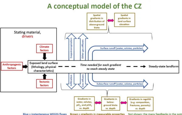
Such difficulties are largely due to two factors: (i) we can-not adequately quantify spatial heterogeneities and tempo-ral variations in the reservoirs and fluxes of water, energy, gas, solutes, and sediment (WEGSS); and (ii) we do not ad-equately understand the interactions and feedbacks among chemical, physical, and biological processes in the CZ that control these fluxes. This latter problem reflects the fact that the CZ (Fig. 1) is characterized by tight coupling between chemical, physical, and biological processes that exert both positive and negative feedbacks on surface processes. Mod-eling the CZ is fraught with problems precisely because of these feedbacks and because the presence of thresholds means that extrapolation from sparse measurements is chal-lenging (Chadwick and Chorover, 2001; Ewing et al., 2006). However, the result of these couplings and feedbacks is that patterns of measurable properties emerge during evolu-tion of critical zone systems that are repeated from site to site despite variations in environmental conditions. Such patterns include the distributions across landscapes or versus depth of such observables as regolith, fractures, bacterial species, or gas composition. Gradients in some important observable properties (e.g., surface elevation, chemistry of water, and regolith composition) emerge as indicators of the evolution of the CZ and reveal aspects of the underlying complex be-havior (brown boxes, Fig. 1). For systems experiencing neg-ative feedbacks, such gradients are thought to move toward
steady-state conditions, i.e., gradients that remain constant over some interval of time.
In Fig. 1, some of these important gradients are arrayed from left to right to indicate the increasing length of time it takes for each gradient in general to achieve such a steady state. In other words, a steady-state soil gas depth pro-file might develop more rapidly than a steady-state regolith chemistry depth profile. Different disciplines tend to focus on different emergent properties (for example, different gra-dients) and thus tend to emphasize processes operating on disparate timescales. However, CZ science is built upon the hypothesis that an investigation of the entire object – the CZ – across all timescales under transient and steady-state condi-tions (Fig. 1) will yield insights that disciplinary-specific in-vestigations cannot. In turn, such integrative study and mod-eling should allow a deeper understanding of the patterns that characterize the CZ.
Given that the mechanisms driving CZ change range from tectonic forcing over millions of years to glacial–interglacial climate change over thousands of years to the recent influ-ence of humans on the landscape, building a model of the CZ is daunting, and no single model has been developed. Instead, suites or cascades of simulation models have been used to address important processes over different timescales (e.g., Godderis and Brantley, 2014). To enable treatment us-ing such a suite of models, each settus-ing for CZ research, in-cluding CZ observatories (CZOs; White et al., 2015), must grapple with the necessity of measuring the processes on dif-ferent timescales to understand the dynamics and evolution of the system.
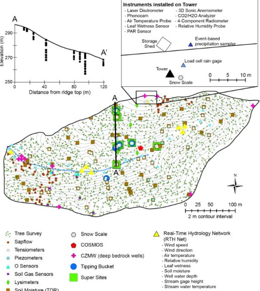
At the Susquehanna Shale Hills CZO (SSHCZO), we have been investigating this challenge by studying the CZ in a 0.08 km2watershed located in central Pennsylvania (the Shale Hills catchment; Fig. 2). At the same time, we have been developing a suite of models that can be intercon-nected to address broad overarching CZ problems (Duffy et al., 2014; Table 1). The focus of the effort has been the small Shale Hills catchment, which was established for hy-drologic research in the 1970s (Lynch, 1976) and was ex-panded with other disciplinary studies as a CZO in 2007 as part of a network of CZOs in the USA. The small spatial scale of Shale Hills allowed the development of a diverse but dense monitoring network that spans disciplines from me-teorology to groundwater chemistry to landscape evolution (Fig. 2). Given the small size, we referred to our measure-ment paradigm as “measure everything, everywhere”. For example, we inventoried all of the∼2000 trees with a di-ameter greater than 20 cm at breast height, drilled 28 wells (up to 50 m deep), sampled soil pore waters at 13 locations at multiple depths approximately every other week during the non-snow-covered seasons for more than 1 year, and mea-sured soil moisture at 105 locations (Fig. 2).
sin-Figure 1.Critical zone science investigates the architecture, character, and dynamics of the earth surface from vegetation canopy to deep groundwater on all timescales. As rock of a certain lithology and structural character is exposed at the earth’s surface due to uplift or erosion, climate-driven inputs transform it to regolith. This transformation, shown in the black box, is catalyzed by biota (a feedback which is not shown explicitly). Gradients of properties describing the CZ are shown in brown boxes. These gradients can become time-independent (steady state) due to the many feedbacks which are not shown. Boxes are placed from left to right to note the increasing duration of exposure time needed to achieve such steady states. For example, depth profiles of regolith composition can become constant when the rate of erosion equals the rate of weathering advance in the presence of feedbacks related to pore water chemistry, soil gas composition, and grain size. The figure emphasizes that gradients to the left can achieve steady state quickly compared to properties to the right. Therefore, properties to the left are often studied as if the properties in boxes to the right are constant boundary conditions. However, over the longest timescales, all properties vary and can affect one another. The complexity of feedbacks (which are not shown for simplicity) can also create thresholds in system behavior. Red boxes indicate drivers and blue arrows are WEGSS fluxes (upward arrows for aboveground and downward arrows for belowground).
Table 1.Designing a suite of CZ models. PIHM: Penn State Integrated Hydrologic Model; LE–PIHM: PIHM with landscape evolution mod-ule; Regolith–RT–PIHM: PIHM with regolith formation and reactive transport modules; CARAIB: CARbon Assimilation In the Biosphere; ED2: Ecosystem Demography model; Flux–PIHM–BGC: PIHM with surface heat flux and biogeochemistry modules; PIHM–SED: PIHM with sediment transport module; RT–Flux–PIHM: PIHM with surface heat flux and reactive transport modules; Flux–PIHM: PIHM with surface heat flux module.
Modeling purpose Model Timescale of interest
Numerical models in use Topography (landscape evolution) LE–PIHM Days–millions of years at SSHCZO Regolith composition and structure Regolith–RT–PIHM, WITCHa Hours–millions of years
Distribution of biota BIOME4b, CARAIBc, ED2 Days–centuries C and N pools and fluxes Flux–PIHM–BGC Days–decades
Sediment fluxes PIHM–SED Hours–decades
Solute chemistry and fluxes RT–Flux–PIHMd, WITCH Hours–decades Soil CO2concentration and fluxes CARAIB Hours–decades Energy and hydrologic fluxes PIHMe, Flux–PIHMf Hours–decades
Geological factor Uplift rate, bedrock composition, bedrock physical properties, preexisting geological factors such as glaciation
External driver Energy inputs, chemistry of wet and dry deposition, atmospheric composition, climate conditions, anthropogenic activities
Figure 2.Mapped summary of the “everything, everywhere” sampling strategy at the Shale Hills subcatchment. Insets show soil moisture sensors (circles) and lysimeters (squares) along the transect shown on the map. Sensor and lysimeter depths are exaggerated 5 times compared to the land surface elevation. Second inset shows instrumentation deployed at the meteorological station on the northern ridge. Small green dots on the map are the trees that were surveyed and numbered: the subcatchment contains a dry oak-mixed hardwood community type (Fike, 1999) with an extremely diverse mix of hardwood and softwood species, including white oak (Quercus alba), sugar maple (Acer
saccharum), pignut hickory (Carya glabra), eastern hemlock (Tsuga canadensis), and chestnut oak (Q. montana). The sparse understory
consists of American hop hornbeam (Ostrya virginiana) and serviceberry (Amelanchier spp.). As we upscale the CZO to all of Shavers Creek, many measurements will be eliminated in the Shale Hills subcatchment as we emphasize only a Ground HOG and Tower HOG deployment as described for the Garner Run subcatchment.
gle lithology (shale), which simplified the boundary condi-tions for models with respect to initial chemical and physi-cal conditions. We have monitored at ridgetops (where water and soil transport is approximately 1-D), along planar hill-slopes (transects where such transport is essentially 2-D), and within swales and the full catchment (where transport must be considered in full 3-D). Where possible, these observa-tions have then been paired with 1-D, 2-D, and 3-D model simulations. Using the conceptualization of 1-D, 2-D, and 3-D settings in the catchment has allowed measurements and modeling to proceed in a synergistic fashion: the reduction in complexity in 1-D and 2-D sites enabled development of
of the catchment, but soil formation models for swales or the entire catchment still remain to be developed.
In contrast to the soil formation models that have targeted the 1-D and 2-D sites, our models of water flow have been de-veloped for the entire catchment (e.g., Qu and Duffy, 2007). In fact, study of an entire catchment with a hydrologic model is sometimes more tractable than for smaller sub-systems be-cause the large-scale study allows a continuum treatment, whereas treatment of smaller-scale sub-systems within the catchment might require measurements of the exact posi-tions of heterogeneities such as fractures, faults, and low-permeability zones.
The goal of the SSHCZO project now is to grapple with some of these down- and upscaling issues by expanding the CZO from Shale Hills to the encompassing 164 km2Shavers
Creek watershed (Fig. 3). The expansion was designed to al-low the investigation of a broader range of lithology (sand-stone, calcareous shale, minor limestone) and land use (agri-culture, managed forest, minor development), and to test models on larger spatial scales. To enable understanding of the larger watershed, we chose to analyze a suite of smaller subcatchments in detail, each of which were selected to be the largest that still drain a single rock unit or land use type. This allows evaluation of how much of our understanding from Shale Hills is transferable to other lithologies with dif-ferent initial conditions but with the same climate. Addi-tionally, we are making targeted measurements of the main stem of Shavers Creek in nested catchments of differing size within the larger watershed, in order to upscale our site-specific models to a relatively complex watershed.
Despite its small size, Shavers Creek contains much of the variability in CZ parameter space found within the Susque-hanna River basin and the Appalachian Valley and Ridge province in general. By measuring in detail paired catch-ments of similar size but different underlying conditions, along with targeted measurements in nested catchments of differing size, we aim to test theories of CZ evolution, param-eterize models (Table 1) in different settings, and explore ap-proaches toward upscaling across different size watersheds.
To understand the interaction of WEGSS fluxes in Shavers Creek and its smaller subcatchments, it is necessary to move beyond the paradigm of measuring everything, everywhere (Fig. 2) to an approach of measuring “only what is needed”. This phrasing, although simplistic, should resonate with any field scientist: the choice of measurement design is at the heart of any field project. But when we study the CZ as a whole, we are asking how one allocates resources to mea-sure and model the dynamics and evolution of the entire CZ system. This paper describes our philosophy of measurement in the CZO; our previous paper describes the modeling ap-proach (Duffy et al., 2014). Obviously, due to the wide range of CZ processes across environmental gradients (Fig. 1), the specifics of our proposed sampling design will differ from such designs at other sites. We nonetheless describe the phi-losophy behind our approach to stimulate focus on the broad
question: how can we adequately and efficiently measure the entire CZ to best learn about its evolution and function? To exemplify our design, we also describe the first part of our ex-pansion from Shale Hills to a sandstone subcatchment within Shavers Creek.
2 Connections between model development and field measurements
The suite of models shown in Table 1 is designed to de-velop understanding over the entire CZ as an integral object of study, i.e., one system. Field measurements are prioritized and driven by data needs for developing models (e.g., Ta-ble 1) and model development is dictated by observations in the field. Hand in hand with this system-level approach, researchers from different disciplines also bring discipline-specific hypotheses to their research that are related to disci-plinary gaps in knowledge. Thus, discidisci-plinary-level hypothe-ses also drive CZO research and sometimes these hypothehypothe-ses feed directly into the overall CZ suite of models. Further-more, because our understanding of the complicated suite of CZ processes is still in its infancy, both baseline measure-ments and curiosity-driven sample collection are still vital to determine the important processes. Throughout, models and observations are allowed to evolve to enable the two-way ex-change of insights needed to maximize CZ science.
Given all the needs for data, the sampling plan which is implemented in a CZO must provide both measure-ments to test disciplinary hypotheses and observations nec-essary to bridge across disciplines. Additionally, certain measurements such as geophysical and remote sensing sur-veys, catchment-integrating stream measurements, and time-integrating analysis of alluvial and colluvial sediments can be made along with model simulations to upscale across space (from limited-point or subregion measurements to the whole watershed) and time (from limited temporal measurements to geological timescales).
Perhaps the largest difficulty inspatiallycharacterizing the CZ in any observatory is the assessment of the extremely het-erogeneous subsurface and land surface, ranging from the as-sessment of regolith and pore fluids down to bedrock to vari-ations in land use. Because the mixing timescales of biota, regolith, and bedrock are relatively slow (compared to mix-ing of atmospheric and surface water reservoirs), the assess-ment of the spatial distribution of biota, regolith, and bedrock properties is both important and extremely challenging (Niu et al., 2014). On the other hand, rapid changes in the at-mospheric reservoir make robust atat-mospheric measurements technically difficult. The hydrologic state is intermediate, ex-hibiting large spatial and temporal variability.
Figure 3.Map of Shavers Creek watershed, highlighting(a)topography derived from airborne lidar,(b)geology (Berg et al., 1980), and (c)land use (Homer et al., 2015). In moving from “measure everything everywhere” (our paradigm in the 8 ha Shale Hills catchment; SH) to “measure only what is needed” in the Shavers Creek watershed (164 km2), we chose to investigate two new first-order subcatchments: a forested sandstone site (along Garner Run, marked GR) and an agricultural calcareous shale site (to be determined). In addition, three sites on Shavers Creek have been chosen as stream discharge and chemistry monitoring sites (marked SCAL – Shavers Creek above lake; SCBL – Shavers Creek below lake; and SCO – Shavers Creek outlet). Location of Fig. 4 is indicated by cross section A–A’.
were largely related to hillslope position, colluvium related to the Last Glacial Maximum (LGM), fracturing, differences in sedimentary layers, and relatively limited spatial variations in vegetation. To understand the CZ at the Shavers Creek wa-tershed, on the other hand, we must grapple with a more com-plex set of variations related to differences in lithology, land
use, climate change, and landscape adjustment to changes in base level due to tectonics, eustasy, or stream capture (Fig. 3). Here, the term base level refers to the reference level or eleva-tion down to which the watershed is currently being eroded.
ran-dom but rather to be stratified based on geological and ge-omorphological knowledge. An implicit hypothesis underly-ing this approach is the idea that samplunderly-ing can be more lim-ited for a stratified approach based on geological (especially geomorphological) knowledge. For example, a first-order ob-servation about hillslope morphology in Shale Hills based on long-standing observations from hillslope geomorphology is the delineation between planar slopes and swales: the former experience largely 2-D nonconvergent flow, while the latter experience 3-D convergent flow of water and soil. Where many randomly chosen soil pits might be necessary if the delineation of swales versus planar hillslopes was ignored, when representative pits are dug to investigate these features separately, the number of pits can be minimized.
Another aspect of our stratified sampling plan is to com-plement measurements at Shale Hills by targeted measure-ments in two new subcatchmeasure-ments of Shavers Creek chosen to represent two of the new lithologies in the watershed. Once again the stratification of the sampling design is dictated by geological knowledge: bedrock geology is known to exert a first-order control on WEGSS fluxes in the CZ (e.g., Duvall et al., 2004; Williard et al., 2005). The first such new sub-catchment is forested and underlain only by sandstone. The second subcatchment for targeted measurements is currently being identified on calcareous shale. This second subcatch-ment will also host several farms and will allow the assess-ment of the effects of this land use on WEGSS fluxes.
To upscale from subcatchments to Shavers Creek, the targeted subcatchment data will be amplified by measure-ments of chemistry and streamflow along the main stem of Shavers Creek as well as catchment-wide meteorologi-cal measurements (Fig. 3). The upsmeteorologi-caling will rely on the small number of sites chosen for soil, vegetation, pore-fluid, and soil gas measurements in each subcatchment. To extrapo-late from and interpoextrapo-late between these limited land surface measurements, models of landscape evolution (LE–PIHM), soil development (e.g., Regolith–RT–PIHM, WITCH), dis-tribution of biota (BIOME4, CARAIB), C and N cycling (Flux–PIHM–BGC), sediment fluxes (PIHM–SED), solute fluxes (RT–Flux–PIHM, WITCH), soil gases (CARAIB), and energy and hydrologic fluxes (PIHM, Flux–PIHM) will be used. In effect, the plan is to substitute everything every-where with measurements of only what is needed by using (i) integrative measurements (geophysics, lidar, stream, at-mosphere), and (ii) models of the CZ. As a simple exam-ple, a regolith formation model is under development that will predict distributions of soil thickness on a given lithol-ogy under a set of boundary conditions. Since much of the water flowing through the upland catchments under study in the CZO flows as interflow through the soil and upper frac-tured zone (Sullivan et al., 2016), use of the regolith for-mation model will enable better predictions of the distribu-tion of permeability. Of course, the models will be contin-ually groundtruthed against pinpointed field measurements.
With this approach, water fluxes in the subcatchments and in Shavers Creek watershed itself will eventually be estimated. For clarity in describing the measurements in each sub-catchment that are needed for the models, we have given names to arrays of instruments (Table S1 in the Supplement). The array of instruments in soil pits (1 m×1 m× ∼2 m deep) and in trees near the pits along a catena is referred to as ground hydrological observation gear (Ground HOG). The Ground HOG deployments also are the locations for as-sessments of vegetation across transects. Geophysical sur-veys and geomorphic analysis using lidar are conducted to interpolate between or extrapolate beyond the catenas.
In addition to Ground HOG, the energy, water, and car-bon fluxes are measured using tower hydrologic observation gear (Tower HOG). Ground and Tower HOGs are in turn ac-companied by measurements of chemistry and temperature of stream and groundwater, as well as discharge and water level for stream and groundwater, respectively. As discussed above, these streams and groundwaters provide natural spa-tial and temporal integrations over the watershed and there-fore provide constraints on the 3-D-upscaled models.
Data from Ground HOG and Tower HOG will be used to parameterize and constrain model–data comparison and data assimilation. In fact, the choice of targeted measure-ments is derived at least in part from an observational sys-tem simulation experiment (OSSE) completed for the Shale Hills catchment using the Flux–PIHM model (Table 1) (Shi et al., 2014b). The OSSE evaluates how well a given obser-vational array describes the state variables that are targeted by Flux–PIHM. Specifically, this OSSE (Shi et al., 2014b) emphasized water and energy fluxes for the catchment.
Prior to the OSSE, a sensitivity analysis was performed (Shi et al., 2014a) to determine the six most influential model parameters that were needed to constrain and produce a suc-cessful simulation. We defined “sucsuc-cessful simulation” as one that reproduced the temporal variations of the four land surface hydrologic fluxes (stream discharge, sensible heat flux, latent heat flux, and canopy transpiration) and the three state variables (soil moisture, water table depth, and surface brightness temperature) (Table 1) with high correlation co-efficients and small root mean square errors. Once the six most influential model parameters were determined – poros-ity, van Genuchten parametersαandβ, Zilitinkevich param-eters, minimum stomatal resistance, and canopy water stor-age – the OSSE was then performed.
On the basis of this OSSE, we are targeting mea-surement of stream discharge, soil moisture, and surface brightness temperature for each of the SSHCZO subcatch-ments on shale, sandstone, and calcareous shale. These measurements should allow us to reproduce subcatchment-averaged land–atmosphere fluxes and subsurface hydrol-ogy adequately. Once the three subcatchments are param-eterized, the models will then be upscaled to the entire Shavers Creek watershed using information from lidar, the Natural Resources Conservation Service Soil Survey Geo-graphic database (SSURGO; http://www.nrcs.usda.gov/wps/ portal/nrcs/main/soils/survey/), geological maps, geophysi-cal surveying, and land use.
Currently, the OSSE has only been used for assimilation of water and energy data but is being expanded to include biogeochemical variables. We also aim to complete an OSSE for C and N fluxes in each subcatchment. In the long run, we could also extend the OSSE to assimilate data for other solutes and for sediments.
Modeling results from Shale Hills indicated that an accu-rate simulation of the subcatchment spatial patterns in soil moisture was achieved using a relatively limited set of hydro-logic measurements made at a few points (Shi et al., 2015a). Specifically, we had to measure (i) stream discharge at the outlet, (ii) soil moisture at a few locations, and (iii) ground-water levels at a few locations. The soil moisture (ii) and groundwater (iii) data used to calibrate the model were from three nearly colocated sites in the valley floor. These real-time hydrology network sites (referred to as RTHnet in Fig. 2) were the only sites with continuous data at the time of model calibration (data from the Cosmic-ray Soil Mois-ture Observing System (COSMOS)) were not yet available). The measurements were averaged across the three RTHnet sites (see data posted at http://criticalzone.org/shale-hills/ data/dataset/3615/) to provide one calibration point in the model. Extending from this calibration point to the en-tire catchment was attempted using data from SSURGO. However, because of the coarse spatial data available in SSURGO, this was not successful for the very small Shale Hills catchment. Therefore, porosity, horizontal and vertical saturated hydraulic conductivity, and the van Genuchten pa-rametersαandβ were separately measured for each soil se-ries and then were averaged for the whole soil column for each soil series (Table S2). These soil core measurements for each soil series were used to constrain the shape of the soil water retention curve for each soil series in the model.
The result of this effort was that for the monolithologic 0.08 km2catchment of Shale Hills, five soil series were iden-tified and soil properties measured (Lin et al., 2006). As we proceed with work on the new subcatchments, one of two approaches will be used. First, it is possible that rela-tively few soil moisture measurement locations are required in any given catchment, as long as we can obtain soil hy-draulic properties for each soil series. Using the SSURGO soils database, such measurements could be made to
parame-terize the model. Alternatively, spatially extensive soil mois-ture measurements based on COSMOS may be adequate to infer the variations in soil hydraulic properties on a series-by-series basis or based on geomorphological criteria. The over-all plan is to use (i) SSURGO, (ii) geomorphological con-straints, (iii) COSMOS, and (iv) soil moisture measurements along the catenas to parameterize Flux–PIHM.
To the extent possible, we parameterize these PIHM mod-els with data sets and then evaluate the modmod-els with different data sets. The phrase “data assimilation” conveys the idea, however, that with more and more complex models, the data and the model output become harder to distinguish. For ex-ample, the output calculated for a given observable from a complex model may be more accurate than any individual measurement of that observable. As model output is used to parameterize other models, such data assimilation obscures the difference between model and data. Considered in a dif-ferent way, data assimilation provides a means to combine the strengths of both in situ observations and numerical mod-els. Data assimilation can thus provide optimal estimates of observable variables and parameters, taking into account both the uncertainties of model predictions and observations. As new types of observations are provided, we first eval-uate PIHM model output against the new observations prior to calibrations to see if the current calibration predicts the new data. This comparison is ongoing for the Garner Run subcatchment. If the prediction is poor, this yields insight into the capabilities of our model under new conditions. If we discover that even with a new calibration we cannot suc-cessfully predict the new observations, we will incorporate a new module that describes a new phenomenon in PIHM. For example, discrepancies between model output and prelimi-nary observations at Garner Run have led us to hypothesize that the distribution of boulders on the land surface – a phe-nomenon not observed in the Shale Hills catchment – must be incorporated into the PIHM models. By tracking which pa-rameters must be tuned and which processes must be added, we gain insights into both the model and system dynamics, and we learn which parameters must be observed if we want to apply our model to a new site or a new time period.
3 Implementation in the Garner Run subcatchment
Figure 4.Geologic cross section of Garner Run subcatchment reproduced from Flueckinger (1969). Map units include Mifflintown (Middle Silurian), Clinton group (including Rose Hill formation), Tuscarora (Lower Silurian), and Juniata (Upper Ordovician). Cross section position is downstream from the Garner Run subcatchment (see Fig. 3) and locally preserves Clinton Group shales in the valley floor, overlying the Tuscarora Formation.
3.1 Geologic, geomorphic, and land use context of Garner Run
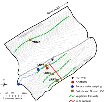
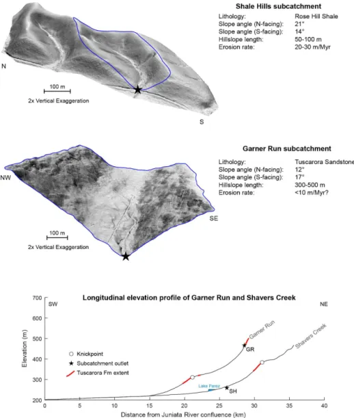
A central underlying hypothesis of SSHCZO work is that the use of geomorphological and land use analysis can in-form sampling strategy so that measurements can be lim-ited in number. Therefore, we start by describing the current knowledge of the geomorphological setting of the Garner Run subcatchment and land use. The subcatchment drains a synclinal valley underlain by the Silurian Tuscarora Forma-tion between the NW–SE trending ridges of Tussey Moun-tain and Leading Ridge (Figs. 3–5). The Tuscarora Forma-tion, which locally consists of nearly pure quartz sandstone with minor interbedded shales, is the ridge-forming unit that caps the highest topography in Shavers Creek watershed. The hillslopes of both Tussey Mountain and Leading Ridge are nearly dip slopes, i.e., the roughly planar hillslopes parallel the bedding in the sandstone (Figs. 4, 5). Indeed, subtle bed-ding planes can be observed in lidar-derived elevation data (Fig. 6b). The strong lithologic control on landscape form is manifested clearly in the high-resolution (1 m) bare-earth lidar topography.
The hillslope morphology of the Garner Run subcatch-ment also contrasts strikingly in several ways from that of Shale Hills. Most notably, the sandstone hillslopes of Tussey Mountain and Leading Ridge are nearly planar in map view: they have not been dissected with the streams and swales common in the shale topography of much of Shavers Creek (Fig. 6). Hillslopes underlain by the Tuscarora Formation are also nearly 10 times longer (300–600 m) than those under-lain by other geologic units within Shavers Creek, includ-ing shales. In Shale Hills, for example, hillslopes are 50– 100 m in length (Fig. 7). Furthermore, the hillslopes at Gar-ner Run are less steep (mean slope: 12–17◦
) compared to those at Shale Hills (mean slope: 14–21◦
), despite having significantly stronger underlying bedrock.
The observation of steeper hillslopes in Shale Hills ver-sus Garner Run is particularly curious given that both sub-catchments are presumed to have experienced similar histo-ries of climate and tectonism. If the two landscapes were in
Figure 5.Map showing Garner Run subcatchment (blue line is the stream). Black dashed lines delineate Harry’s Valley Road. The Harry’s Valley well (HV1) is shown along with the location of the COSMOS unit and the outlet weir (blue dot to the southwest). The blue dot to the northeast indicates the approximate range of surface water sampling that is ongoing. Soil pits have been emplaced as shown, along with the Ground HOG deployment. Location of vege-tation and ground-penetrating radar (GPR) transects reported in this paper are also shown. Tower HOG location is along the crest of Tussey Mountain to the northeast of the Garner Run subcatchment (Fig. 3).
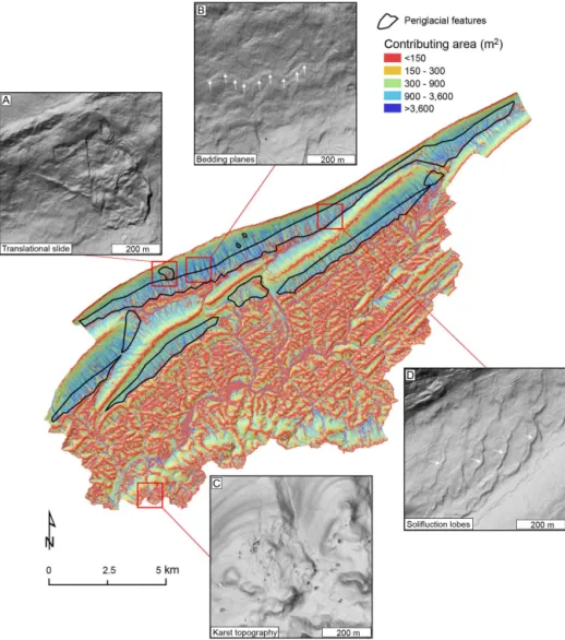
Figure 6.Map of bedrock and periglacial process controls on topography in Shavers Creek watershed. The contributing area was determined using the D-Infinity flow routing algorithm (Tarboton, 1997). The map highlights spatial variations in drainage density that correspond to sandstone (low drainage density and long hillslopes), shale (high drainage density and short hillslopes), and carbonate (intermediate drainage density and hillslope length) bedrock (see Fig. 4). Black outlines correspond to periglacial features expressed in the 1 m lidar topography, such as landslides(a)and solifluction lobes(d). Sandstone bedding planes(b)and limestone karst topography(c)are also prominent.
Two issues may explain this apparent contradiction. First, while the morphology of the Shale Hills catchment bears lit-tle resemblance to the underlying structure of steeply dipping shale beds, the topography of Garner Run is nearly entirely controlled by underlying Paleozoic structure (Fig. 4). Specif-ically, hillslope angles reflect dip slopes rather than morpho-dynamic equilibrium. Second, as a headwater stream in the Shavers Creek watershed, Garner Run is isolated from the regional base level controls that influence downstream catch-ments such as Shale Hills (Fig. 6).
Specifically, analysis of stream longitudinal profiles on Garner Run and the main stem of Shavers Creek reveals prominent knickpoints at elevations of∼320 and 380 m, re-spectively (Fig. 7). Such breaks in channel slope geomorphi-cally insulate the upper stream reaches from the main stem
of Shavers Creek and could be consistent with different rates of local river incision into bedrock in the upper and lower reaches (e.g., Whipple et al., 2013). Published cosmogenic nuclide-derived bedrock lowering rates ranging from 5 to 10 m Myr−1 from similar nearby watersheds (Miller et al.,
2013; Portenga et al., 2013) may be a good estimate for rates in Garner Run upstream of the knickpoint (Fig. 7). These rates are indeed 3–4 times lower than bedrock lowering rates inferred for the Shale Hills catchment (20–40 m Myr−1; Ma
et al., 2013; West et al., 2013, 2014), which lies downstream of the knickpoint on Shavers Creek.
Figure 7.Perspective slopeshade maps (darker shades: steeper slopes) of Shale Hills (top panel) and Garner Run (middle panel) subcatch-ments, emphasizing differences in slope asymmetry and hillslope length. Soil production and erosion rates for Shale Hills subcatchment were measured based on U-series isotopes and meteoric10Be concentrations in regolith, respectively (Ma et al., 2013; West et al., 2013, 2014). Erosion rate for Garner Run subcatchment is estimated based on detrital10Be concentrations from nearby sandstone catchments with simi-lar relief (Miller et al., 2013). Bottom panel shows stream longitudinal profiles, highlighting the lithologic control on knickpoint locations. Note the location of the Shale Hills subcatchment (SH) downstream of the knickpoint on Shavers Creek and the location of the Garner Run subcatchment (GR) upstream of the knickpoint on Garner Run.
stream capture and drainage reorganization (e.g., Willett et al., 2014), or temporal and spatial variations in bedrock ex-posure at the surface (e.g., Cook et al., 2009). Testing these competing controls will require additional direct measure-ments of bedrock lowering rates with cosmogenic nuclides at Garner Run, in addition to bedrock river incision models that can account for both variations in rock strength and tem-poral changes in relative base level.
In addition to variations in structure, lithology, and base level, Quaternary climate variations have left a strong im-print on the landscape of Garner Run and Shavers Creek in general. While the relict of the periglacial processes at Shale
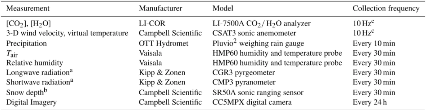
Table 2.Measurements and instrumentation for Tower HOG system.
Measurement Manufacturer Model Collection frequency
[CO2], [H2O] LI-COR LI-7500A CO2/H2O analyzer 10 Hzc 3-D wind velocity, virtual temperature Campbell Scientific CSAT3 sonic anemometer 10 Hzc Precipitation OTT Hydromet Pluvio2weighing rain gauge Every 10 min Tair Vaisala HMP60 humidity and temperature probe Every 30 min
Relative humidity Vaisala HMP60 humidity and temperature probe Every 30 min Longwave radiationa Kipp & Zonen CGR3 pyrgeometer Every 30 min Shortwave radiationa Kipp & Zonen CMP3 pyranometer Every 30 min Snow depthb Campbell Scientific SR50A sonic ranging sensor Every 30 min Digital Imagery Campbell Scientific CC5MPX digital camera Every 24 h
aAll four components of radiation (upwelling and downwelling (longwave and shortwave)) will only be measured at Shale Hills Tower HOG due to the location of the
Garner Run Tower HOG. To model Garner Run we will use the Shale Hills data.bOriginally designed as part of tower system but will be deployed at Leading Ridge valley floor (LRVF) Ground HOG location because the Garner Run tower will be located outside of the catchment.cThe turbulent fluxes (sensible and latent heat) and the momentum flux are computed at 30 min intervals via eddy covariance using these data collected at 10 Hz.
the catchment – Tussey Mountain hillslope – is steeper at the top, has greater relief, retains evidence of past translational slides, and contains open, unvegetated boulder fields. At the foot of the Tussey Mountain hillslope is a strong slope break that demarcates a low-sloping region characterized by abun-dant solifluction lobes, which appear to have accumulated as a large, valley-filling deposit (Figs. 6, 7). Such features were either not as active or their evidence has been erased or buried at the Shale Hills subcatchment.
Many of these geomorphological features have controlled or been imprinted on CZ processes and human activities in Garner Run. For example, the modern flow pathways for sur-face and groundwater in Garner Run are significantly influ-enced by the forcing factors of tectonism, climate, and an-thropogenic activity. Flow pathways are influenced (i) by to-pography inherited from geologic events from 108years be-fore present, (ii) by variations in soil grain size as dictated by periglacial processes operating 104years ago, and (iii) by modern land use over the last 102–103years.
In terms of land use, the influence of anthropogenic activ-ity in the catchment is relatively minor and consistent with the surrounding region. Neither Shale Hills nor Garner Run subcatchments show signs of having been plowed or farmed in row-crop agriculture, although some grazing may have oc-curred. The top of one of the ridges in Shale Hills appears to define a field edge. Both subcatchments were forested for at least 100 years. Based on historic aerial photographs, both watersheds contained intact, closed canopy forests in 1938 and show no sign of obvious stand level disturbance since that year. In the mid 1800s, significant quantities of char-coal were made in this region to run several nearby iron fur-naces. Given that charcoal hearths have been identified in the subcatchments from lidar, the subcatchments were probably cleared in the mid to late 1800s as most available wood was used for charcoal making. This land use was also often asso-ciated with fires.
This short analysis of the geomorphology and land use highlights the influence of the forcing mechanisms (tecton-ism, climate, anthropogenic activity) that operate over a wide range of timescales and yet influence modern CZ processes. The CZO efforts document the importance of providing geo-logic and geomorphic context for investigation of the CZ.
3.2 Water and energy flux measurements at Garner Run: Tower HOG
Surface energy balance measurements (eddy covariance measurements of sensible and latent heat fluxes or upwelling terrestrial radiation or skin temperature) are needed to con-strain Flux–PIHM (Shi et al., 2014b). Measurements of pre-cipitation, atmospheric state, and incoming radiation are needed as inputs to the model. These measurements provide the data needed to simulate the catchment hydrology that is critical to understanding today’s WEGSS fluxes. In addition, these fluxes are drivers for millennial-timescale landscape evolution (Fig. 1).
Instrumentation for measurements of water and energy flux measurements are designed as part of the “tower hydro-logical observation gear” – referred to here as Tower HOG (Tables 2 and S1). Precipitation will be measured near Gar-ner Run on a road crossing Tussey Mountain that is also the site of a preexisting communications tower (see Fig. 3). A disdrometer (LPM, Theis Clima GmbH) and weighing rain gauge have been in use at Shale Hills since 2009 and 2006, respectively, to measure precipitation. To measure precipita-tion amount at Garner Run, we are installing a simpler instru-ment (Pluvio2, OTT Hydromet weighing rain gauge). Mea-surements will be compared to the National Atmospheric Deposition Program (NADP) measurements and samples of rainwater. According to the nearest NADP site, Garner Run receives 1006 mm year−1precipitation with an average pH of
5.0 (Thomas et al., 2013).
tower on the Tussey Mountain ridgeline (Fig. 3). Although located outside of the subcatchment, the measurement foot-print for the tower will be sensitive to fluxes from forests representative of those in Garner Run. The complex terrain at Shale Hills and Garner Run makes eddy covariance mea-surements difficult to interpret in stable micrometeorological conditions. Since the primary energy partitioning happens during the day when the atmosphere is typically unstable, daytime sensible and latent heat flux measurements are suffi-cient to constrain the hydrologic modeling system. Daytime carbon dioxide flux measurements will inform the biogeo-chemical modeling system.
3.3 Vegetation mapping
Vegetation impacts today’s WEGSS fluxes and is known to have influenced regolith formation and sediment transport over geologic time. As we study subcatchments to under-stand budgets, we seek to learn enough about vegetation to extrapolate WEGSS fluxes to the Shavers Creek watershed. As described below, we once again use the geomorphological framework to design the measurement strategy for vegeta-tion. We also want to understand the biogeochemical controls on fluxes of nutrients such as nitrate out of Shavers Creek. Ultimately, an OSSE will be run to compare measurements to model predictions as a way to determine the important pa-rameters for predicting carbon and nitrogen fluxes. It may also be necessary to determine the effect of individual tree species on N flux (Williard et al., 2005).
As part of the geomorphological measurement strategy, we mapped the vegetation in Garner Run subcatchment across the Ground HOG catena (ridge top, midslope, and valley floor positions on one side of catchment and one midslope site on the other side; Fig. 5). The objective of the catena-based stratified sampling design was to measure spatial vari-ability in vegetation, under the assumption that landscape position was an important control on vegetation. These mea-surements set the stage for planned remeamea-surements to under-stand temporal variability. For example, future assessments will quantify aboveground biomass, an important carbon pool. Variability in forest composition, standing biomass, and productivity across a watershed is generally related to gradients in biotic and abiotic resources such as soil chem-istry or structure, water flux, and incoming solar energy. Therefore, the relatively restricted vegetation analysis design (Fig. 5) will be upscaled based on the team’s developing knowledge of the distribution of soils across the watershed as well as lidar-based estimates of tree biomass and seasonal patterns of leaf area index and tree diameter growth. Given that we have not yet run an OSSE for C or N fluxes, our mea-surements of vegetation are relatively broad to enable such future analysis.
Vegetation measurements are important not only for C and N fluxes but also for water flux. At Shale Hills, seasonal variation in tree transpiration has been estimated using tree
sap flux sensors (Meinzer et al., 2013). While we sampled many different tree species in multiple locations at Shale Hills (Fig. 2), a more restricted number will be sampled at Garner Run. For example, sap flux sensors are planned for only the midslope positions of Ground HOG (Fig. 5). While eddy flux and soil moisture dynamics provide estimates of total transpiration and evaporation, sap flux provides direct estimates of tree transpiration that can constrain model pre-dictions of transpiration. Collectively, these measures will help evaluate Flux–PIHM model processes. In addition, all approaches to measuring water fluxes are imperfect; errors can best be constrained when multiple approaches are used.
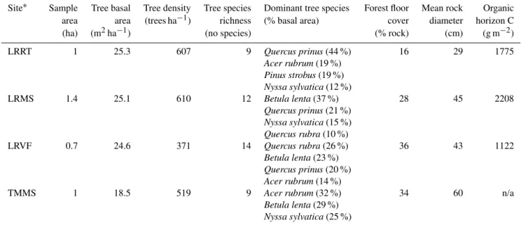
In addition to these sap flux measurements limited to mids-lope pits, vegetation has been sampled in linear transects par-allel to the slope contour at each of the four soil pits (Fig. 5; Sect. 3.4), i.e., at Leading Ridge ridge top (LRRT), Lead-ing Ridge midslope (LRMS), LeadLead-ing Ridge valley floor (LRVF), and Tussey Mountain midslope (TMMS). Each veg-etation transect was 10 m along the direction perpendicular to the valley axis and∼700–1400 m parallel to the valley axis. Measurements along the transects yielded vegetation and forest floor cover data for 4.1 ha in the subcatchment (Ta-ble 3). The transects provide vegetation input data for land surface hydrologic models and also evaluation data for a spatially distributed biogeochemistry model (Flux–PIHM– BGC; Table 1). In the transected area, 2241 trees > 10 cm di-ameter at breast height were measured, mapped, and perma-nently tagged. Understory vegetation composition was mea-sured at 5 m intervals along transects, and coarse woody de-bris was measured in 25 m planar transects parallel to the main transect, spaced every 100 m. Forest floor cover was classified as rock (typically boulder clasts from periglacial block fall), bare soil, or leaf litter every 1 m along each tran-sect, and the dimensions (a,b,caxes) of the five largest ex-posed rocks were recorded every 25 m. Forest floor biomass was measured every 25 m along transects by removing the organic horizon from a 0.03 m2area for laboratory analysis: samples were dried, weighed, and measured for carbon loss on ignition.
The transect observations document variations in vegeta-tion along the catena (Table 3), as well as spatial variavegeta-tion in vegetation at each position. For example, mean tree basal area (BA; the ratio of the total cross-sectional area of stems to land surface area) in the LRRT transect is 25.3 m2ha−1with
measurements ranging from 0 to 79 m2ha−1. The
subcatch-ment contains a dry oak-heath community type (Fike, 1999), primarily consisting of chestnut oak (Q. montana), red maple (Acer rubrum), black birch (Betula lenta), black gum (Nyssa sylvatica), and white pine (Pinus strobus) in the overstory, with a thick heath understory of mountain laurel (Kalmia lat-ifolia), blueberry (Vaccinium sp.) and huckleberry ( Gaylus-sacia sp.) species, and rhododendron (Rhododendron maxi-mum) along Garner Run.
Table 3.Vegetation sampling in the Garner Run subcatchment.
Site∗ Sample Tree basal Tree density Tree species Dominant tree species Forest floor Mean rock Organic
area area (trees ha−1) richness (% basal area) cover diameter horizon C
(ha) (m2ha−1) (no species) (% rock) (cm) (g m−2)
LRRT 1 25.3 607 9 Quercus prinus(44 %) 16 29 1775
Acer rubrum(19 %)
Pinus strobus(19 %)
Nyssa sylvatica(12 %)
LRMS 1.4 25.1 610 12 Betula lenta(37 %) 28 45 2208
Quercus prinus(21 %)
Nyssa sylvatica(15 %)
Quercus rubra(10 %)
LRVF 0.7 24.6 371 14 Quercus rubra(26 %) 36 43 1122
Betula lenta(23 %)
Quercus prinus(20 %)
Acer rubrum(14 %)
TMMS 1 18.5 519 9 Acer rubrum(32 %) 34 60 n/a
Betula lenta(29 %)
Nyssa sylvatica(25 %)
∗LRRT: Leading Ridge ridge top; LRMS: Leading Ridge midslope; LRVF: Leading Ridge valley floor; TMMS: Tussey Mountain midslope. Measurements were made in
linear belt transects 700–1400 m long and 10 m wide centered at each soil pit position (Fig. 5).
and observations are showing is important in the new sub-catchment: the fraction of land surface covered by boulders. At LRRT, 16 % of points sampled every meter fell on rock. Furthermore, rock coverage at some transect points was as high as 100 % or as low as 0 %. Vegetation and surface rock-iness data from transects will be combined with a suite of ground and remotely sensed measurements from the water-shed such as slope, curvature, aspect, solar radiation, and soil depth to model vegetation dynamics from environmen-tal conditions and interpolate vegetation structure in areas of the watershed not directly sampled. Future remeasure-ments along transects will allow assessment of carbon up-take in vegetation, as well as changes in forest composition and structure.
Additional key vegetation parameters will be assessed at the soil pits described in Sect. 4.4 and Table S2. These addi-tional measurements include root distributions, leaf area in-dex (LAI; described in the next paragraph), litter fall, tree diameter growth, and tree sap flux. Root distributions are being measured at all four soil pits in Garner Run using soil cores to assess the high length densities near the sur-face. Root distributions, combined with soil water deple-tion patterns, can allow the estimadeple-tion of the depth of tree water use over the season. Depth of tree water use, an in-put parameter in the PIHM suite of models, is currently de-rived from a lookup table (http://www.ral.ucar.edu/research/ land/technology/lsm/parameters/VEGPARM.TBL) to deter-mine the rooting depth of each land cover type. We will explore whether the use of field-measured rooting depth as model input improves the modeling of water uptake. In ad-dition, profile wall mapping is being used to analyze the
ar-chitecture, mycorrhizal colonization, and anatomy of deep roots. By characterizing and understanding the controls on root traits along a hillslope, we will eventually be able to use such observations to inform models of both water cycling (Flux–PIHM) and regolith formation (RT–Flux–PIHM; see Table 1).
At weekly intervals in the spring and fall and monthly in-tervals during the summer, LAI will be assessed with a Li-2200 plant canopy analyzer (LI-COR Inc., Lincoln, Nebraska USA). The Moderate Resolution Imaging Spectroradiome-ter (MODIS) also provides remotely sensed 8-day compos-ite LAI (Knyazikhin et al., 1999; Myneni et al., 2002). The MODIS LAI product, however, has a spatial resolution of 1 km2, which cannot resolve the spatial structure in LAI within small watersheds. The product also has a notable bias compared to field measurements (e.g., Shi et al., 2013). The LAI field measurements will be used for detailed informa-tion on leaf phenology, which is an important driver for the modeling of water and carbon fluxes for land surface and hydrologic models (e.g., PIHM, Flux–PIHM; Table 1), and provides calibration or evaluation data for biogeochemistry models like Flux–PIHM–BGC (Naithani et al., 2013; Shi et al., 2013).
assess-ment. One of the key model outputs of Flux–PIHM–BGC is NPP, which can be evaluated using these measured data.
3.4 Soil pit measurements and Ground HOG instrumentation
3.4.1 Soil observations
The uplands of the Garner Run subcatchment land surface falls into one of three categories: (i) fully soil mantled with few boulders emerging at the ground surface, (ii) boulder-covered with tree canopy, and (iii) boulder-boulder-covered without tree canopy. The coarse blocks of the Tuscarora sandstone range in diameter from∼10 to 200 cm, making it challeng-ing to excavate large soil pits (Table 3). To assess the spatial heterogeneity of soils in the Garner Run subcatchment, we therefore focused efforts on four soil pits: three on the north-facing planar slope of Leading Ridge (LRRT, LRMS, LRVF) and one midslope pit on the south-facing slope of Tussey Mountain (TMMS) (Fig. 5). Three pits were dug by hand un-til deepening was impossible (LRRT, LRMS, and TMMS). The LRVF pit was dug by hand and then deepened using a jackhammer until the inferred contact with intact bedrock was reached. The pits were excavated in the following soil se-ries: TMMS, LRRT, and LRMS (Hazleton–Dekalb associa-tion, very steep), and LRVF (Andover extremely stony loam, 0–8 % slopes). This deployment of observations in soil pits along a catena, with an additional pit on the opposite valley wall, is here referred to as Ground HOG (Fig. 5 and Figs. S1, S2 in the Supplement) and is the result of our focus on a min-imalist sampling design.
This design was informed by observations at Shale Hills and the new subcatchment and by modeling conceptualiza-tions. As discussed earlier, the Shale Hills subcatchment up-land up-land surface falls into one of two categories: hillslopes or swales. In contrast, we observed little evidence for swales in Garner Run. All four pits in the new subcatchment were therefore located on roughly planar or somewhat convex-up hillslopes (see below). The rationale for the positions of the pits is as follows. First, regolith formation at a ridge top is the simplest to understand and model (see, for example, Lebe-deva et al., 2007, 2010) because net flux of water is largely downward and net earth material flux is upward over ge-ological time. We are now developing Regolith–RT–PIHM to simulate regolith development quantitatively for such 1-D systems, using constraints from cosmogenic isotope analysis (Table 1). The next level of complexity is a convex-upward but otherwise planar hillslope. The intent for Regolith–RT– PIHM is that it will be able to model hillslopes as 2-D sys-tems (e.g., Lebedeva and Brantley, 2013). Soil pits along a convex-upward but otherwise planar hillslope such as those described for Shale Hills (Jin et al., 2010) can be used to pa-rameterize both 1-D and 2-D models of regolith formation. Third, while both planar hillslopes and swales are impor-tant at Shale Hills (Graham and Lin, 2010; Jin et al., 2011;
Thomas et al., 2013) the lack of swales at Garner Run allows focus on just one catena in the minimalist design. (In fact the lack of swales in the sandstone catchment is one of the ob-servations that we hope we can eventually explain). Finally, the importance of aspect in soil development and WEGSS fluxes has been noted on shale at Shale Hills (Graham and Lin, 2010, 2011; Ma et al., 2011; West et al., 2014), as well as on sandstones in Pennsylvania (Carter and Ciolkosz, 1991). For that reason, Ground HOG includes one pit on the north-ern side of the catchment (Fig. 5).
We will use numerical models to explore regolith forma-tion and to extrapolate to other hillslopes within Shavers Creek watershed. This highlights the importance of under-standing the soil to the CZ effort. Soil provides a record of both transport of rock-derived material as well as fluxes of water over the period of pedogenesis. For example, the pits at Garner Run are characterized from the land surface down-ward by a thin organic layer, a rocky layer, a leached layer characterized by sand-sized grains with few large clasts, a sandy mineral soil with a thin layer of accumulated organic and sesquioxide material, and a deeper clay-rich layer with larger interspersed rock fragments (Fig. S3; Table S2). Depth intervals of the soil every 10 cm and from basal rocks show variations in chemistry (Tables S3, S4) and are being ana-lyzed for grain size, organic matter, and mineralogy.
These soil observations yield further clues to the his-tory of the landscape. The Garner Run subcatchment has been mapped to lie on Lower Silurian Tuscarora sandstone (Flueckinger, 1969). Interpreted as reworked beach sedi-ments (Cotter, 1982), this sandstone has been metamor-phosed to a highly indurated quartzite. Bulk compositions of five rocks collected from the bottom of the five Ground HOG pits were averaged to estimate composition of the protolith (Table S3). These samples contain > 96 wt% SiO2, very
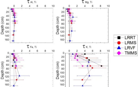
sim-ilar to published Tuscarora compositions (Cotter, 1982). Mi-nor titanium (Ti), generally present in sandstones in highly insoluble minerals, was present in the parent (Table S3) and at even higher concentration in soils (Table S4). This enrich-ment in soil could be due to several processes during weath-ering: for example, retention of Ti from the protolith, losses of elements other than Ti, or addition of Ti to the soil. If Ti in the soil was derived from protolith, loss or gain of other elements in the sandstone can be calculated from the mass transfer coefficient,τij, whereiis Ti andjis an element that was lost or gained (Anderson et al., 2002; Brimhall and Di-etrich, 1987). Assuming the Ti in soil was derived from the protolith,τT i,j values equal 0 within error for Al, Mg, and Fe, indicating that they were neither added nor depleted com-pared to Ti. In contrast,τT i,K> 0, consistent with addition of K to the soil (Fig. 8). Error bars on many of the elements are very large because of the variability in the low concentrations of all elements except Si and O.
Figure 8.Plots of normalized concentration (τ) versus depth for soils analyzed from the four Garner Run subcatchment soil pits (LRVF, LRMS, LRRT, TMMS).Yaxis indicates the depth below the organic–mineral horizon interface.τis the mass transfer coefficient determined using parent composition estimated as the average of five rocks (Table S3) from the bottom of several of the pits based on the assumption that Ti derives from protolith and is immobile. If parent is correctly estimated,τ= −1 when an element is 100 % depleted,τ=0 when no loss or gain has occurred, and isτ >0 when the element has been added to the profile compared to Ti in the parent material.
on hillslopes likely developed not only from rock in place but also from colluvium (Fig. 5). Furthermore, previous re-searchers have pointed out that soils in central Pennsylvania commonly show a brown-over-red layering that may indicate two generations of weathering, i.e., a previously weathered red layer which was then covered by a colluvial layer that ex-perienced additional weathering (the brown layer) (Hoover and Ciolkosz, 1988). Although the soils here did not show a strong brown-over-red color signature (Fig. S3), clay-rich soil at depth may document soil formation before the LGM (Table S2). The addition of K to the soils, even in the resid-ual soils at the ridgetop (Fig. S3), is another complexity. K could have been added as exogenous dust inputs which were very important during and immediately after glacial periods (Ciolkosz et al., 1990). Alternatively, K-containing clay par-ticles could have percolated downward from weathering of the overlying units such as the Rose Hill shale before it was eroded away (Fig. 4). Such movement of fines downward from the Rose Hill have been observed at Shale Hills (Jin et al., 2010): such particles could have been added to the un-derlying Tuscarora and then retained in the soil. In that case, the assumed protolith composition could be erroneous, espe-cially if Ti was added from the downward infiltrating fines. K enrichment could also be explained by shales within the Tuscarora formation itself (Flueckinger, 1969). If these in-terfingered shales were the protolith of the observed soils, this would mean that our estimated protolith composition was K-deficient. Thus, soil analysis (Fig. 8) leads to inter-esting hypotheses that will be investigated.
3.4.2 Ground HOG
The Ground HOG instrumentation enables the in situ mea-surement of soil moisture and temperature, as well as gas and pore-fluid compositions, all at multiple depths (Figs. 5, S2). Ground HOG complements the atmospheric measurements at Tower HOG (Sect. 3.2). Because Ground HOG sites are difficult to access, measurements were automated to the ex-tent possible. However, the lack of access to electricity and the cost of automated sensors (for CO2for example) meant
that a completely automated monitoring system was unfeasi-ble as well. Therefore, our final approach (Fig. S2) included a few automated components recording a continuous time se-ries of data, coupled with additional components to be mon-itored manually but with lower temporal resolution.
“D-20”). At these four depths we installed one to four component devices of the Ground HOG in each pit.
Automated soil moisture and temperature sensors (Hy-dra Probe, Stevens Water Monitoring Systems, Inc. Portland, OR) were emplaced to monitor at 10, 20, and 40 cm depths on the uphill face of each pit (Fig. S2). In addition, time-domain reflectrometry (TDR) waveguides (Jackson et al., 2000) for manual point estimates of soil moisture were in-stalled at the same depths plus D-20 on the uphill pit face and the left and right pit faces (facing uphill). Waveguides are paired metal rods on a single cable that conduct a signal for time-domain reflectometry. The rods are 20 cm long and handmade (Hoekstra and Delaney, 1974, Topp et al., 1980; Topp and Ferre, 2002). We placed 12 (four depths and three pit faces) in each pit. The automated sensors were emplaced at depths expected to have the most dynamic soil moisture. In contrast, the waveguides measure deep soil moisture where temporal variability is expected to be low. The use of waveg-uides added spatial replication at all depths (Figs. 5, S2).
Colocated with every soil moisture waveguide is an ac-cess tube to sample soil gas for measurements of the depth distribution of CO2and O2at a low temporal frequency. At
20 cm below the soil surface and 20 cm above the bottom of the uphill face of the pit, sensors are continuously mea-suring soil CO2 (GP001 CO2 probe, Forerunner Research,
Canada) and O2(SO-110 Sensor, Apogee Instruments, Utah,
USA) at the two midslope catena positions. We selected the midslope catenas for these sensors because they provide the best locations for contrasting north and south aspects. We placed one sensor at the D-20 location to document controls on acid and oxidative weathering near the bedrock interface. The second sensor is near the surface to monitor a zone of high biological CO2 and O2 processing. We did not install
the sensors at the shallowest depth (10 cm) because we found that high diffusion and advection at shallower depths causes the gas concentrations at 10 cm to reflect atmospheric condi-tions, providing less information on soil biology (Jin et al., 2014; Hasenmueller et al., 2015).
Lysimeters (Super Quartz, Prenart Equipment ApS, Den-mark) have been emplaced to allow periodic manual sam-pling of soil pore water for chemical analysis at 20 and D-20 cm depths in all catena locations. The rationale for these depths is the same as described above for the automated CO2
and O2 sensors (they are colocated in the midslope pits).
Overall, these Ground HOG measurements will parameter-ize the regolith formation models (Table 1) and will be used to test hypotheses linking hydrology, biotic production and consumption of soil gases, and weathering rates.
3.5 Upscaling from the pits to the catena using geophysics
To supplement the Ground HOG observations, we use geo-physical and large-footprint methods to interpolate between and extrapolate beyond soil pits. For example, a cosmic-ray
neutron detector (CR-1000B, Hydroinnova Inc.) has been emplaced to measure large-scale (∼0.5 km radius) average soil moisture every 30 min. This COSMOS unit, already used in a variety of ecosystems (Zreda et al., 2013), will measure spatially averaged (3-D) soil moisture content within the wa-tershed. Data processing methods have been developed that accounts for various types of moisture storage (e.g., canopy storage, snow, water vapor; Franz et al., 2013; Zweck et al., 2013). The sensor has been installed near the LRVF pit to provide spatially averaged moisture estimates across the val-ley.
The COSMOS fills in the gap between small-scale point measurements (Fig. 5) and large-scale satellite remote sens-ing. The footprint of COSMOS is optimal for hydrometeoro-logical model calibration and validation in small watersheds. One sensor was installed at Shale Hills in 2011, and we are currently testing the COSMOS data with PIHM. We antici-pate that the results from both catchments will yield insights into the capabilities of cosmic-ray moisture sensing technol-ogy in steep terrain and will offer insights into the problem of upscaling soil moisture measurements.
Ground HOG measurements will be further comple-mented by geophysical mapping along the catenas, includ-ing ground-penetratinclud-ing radar (GPR) transects of subsurface structure. Electromagnetic induction (EMI) mapping of soil electric conductivity will similarly be used to measure soil spatial variations between pits. We plan repeated GPR and EMI surveys, in combination with terrain analysis using li-dar topography, to identify subsurface hydrological features and soil distribution using published procedures (Zhu et al., 2010a, b). We will also field-check regolith depths using augers, drills, etc. With repeated geophysical surveys over time (e.g., different seasons and/or before and after storm events), we can also explore temporal changes in hetero-geneous soilscapes and subsurface hydrologic dynamics, as demonstrated at Shale Hills (Guo et al., 2014; Zhang et al., 2014).
Such geophysical mapping is necessary to link between and compare with soil pit point measurements. For exam-ple, depth to bedrock along the catenas will be mapped using the geophysical surveys and compared to pit measurements (Fig. 5). These data can be used for upscaling biogeochemi-cal patterns and processes. For example, we expect that soil depth and soil moisture exert the strongest controls on vari-ation in soil gas concentrvari-ations, as observed in many places, including Shale Hills (Hasenmueller et al., 2015; Jin et al., 2014). Empirical relationships among these variables devel-oped at Ground HOG points can be coupled with catchment scale soil moisture (from COSMOS) and soil depth (from GPR) data to upscale soil gas characteristics to the whole catchment.
Figure 9.Ground-penetrating radar (GPR) transect of the Leading Ridge catena, showing inferred location of bedrock–soil interface (yellow dashed curve). The three soil pits (LRRT, LRMS, LRVF) are indicated by stars, with their observed depth to bedrock indi-cated by red arrow. LRRT and LRMS were dug by hand until refusal and LRVF was dug by hand and deepened with a jack hammer. GPR data are exaggerated 10 times in vertical dimension as compared to surface topography. Summary bedrock depths are tabulated in Ta-ble 4.
the three major monitoring sites (LRVF, LRMS, LRRT) is shown in Fig. 9. Multiple GPR traverses were completed by pulling the antennae along the ground surface. A distance-calibrated survey wheel with encoder was bolted onto these antennae to provide greater control of signal pulse trans-mission and data collection. The survey wheel occasionally slipped in the challenging terrain, resulting in some errors. Relative elevation data were collected as described below along the traverse line to surface-normalize the data.
A traverse line from near Garner Run to the summit was established that ascends Leading Ridge in a nominally west to east direction from ∼494 to ∼588 m a.s.l. (Fig. 9). The
Table 4.Frequency distribution of bedrock depth measurements along GPR transect (Fig. 9).
Depth to bedrock Upper section Lower section
Shallow (< 0.5 m) 0.00 0.00 Moderately deep (0.5–1 m) 0.26 0.04
Deep (1–1.5 m) 0.51 0.48
Very deep (> 1.5 m) 0.24 0.48
dominant soils mapped along this traverse line (Table S2) in-clude Andover, Albrights, Hazleton, and Dekalb. The very deep, poorly drained Andover and moderately well to some-what poorly drained Albrights soils have been reported in general to have formed in colluvium derived from acid sand-stone and shale on upland toe-slope and foot-slope posi-tions. The moderately deep, excessively drained Dekalb and the deep and very deep, well-drained Hazleton soils formed on higher-lying slope positions in residuum weathered from acid sandstone. These soils have moderate potential for pen-etration with GPR.
The traverse line was cleared of debris but the ground surface remained highly irregular with numerous rock frag-ments and exposed tree roots that often halted the movement and caused poor coupling of the antennae with the ground. Flags were inserted in the ground at noticeable breaks in the topography along the traverse line. User marks were inserted on the radar records as the antenna passed these survey flags. Later, the elevations of these points were determined using an engineering level and stadia rod. The elevation data were entered into the radar data files and used to surface-normalize or terrain-correct the radar records.
In this preliminary investigation, the soil–bedrock inter-face was not easy to identify. This was attributed to poor an-tenna coupling with the ground surface in the challenging rocky terrain, noise in the radar records caused by rock frag-ments in the overlying soil, irregular and fractured bedrock surfaces, and varying degrees of hardness in both rock frag-ments and the underlying bedrock. These factors weakened the amplitude, consistency, and continuity of reflections from the soil–bedrock interface. Nevertheless, preliminary results are described below.