THE USE OF TECHNOLOGY IN PORTUGUESE HOSPITALS

(1)

–

THE CASE OF MRI

ANA CLÁUDIA DIAS MENDES CORREIA MOURA

STUDENT NUMBER 414

A Project carried out for the Applied Policy Analysis course, under the supervision of:

Professor Pedro Pita Barros

(2)

1

Abstract

We study the determinants of MRI use across Portuguese NHS hospitals for patients

belonging to specific DRGs.

Using data on individual hospital admissions, we estimate a probit model including

individual-, hospital-, time- and region-specific variables in order to explain the

probability of a patient being sent for MRI.

Results convey

a tightening effect on the hospital’s budget constraint

in the end of each

year. Hospitals seem to account for regional characteristics when defining adoption

patterns. Individual-specific variables are good predictors of MRI use. Measures taken

by the Government only impact the short run. Finally, the gains from an MRI scan, as

far as the probability of death is concerned, occur mainly for less severe patients.

Keywords: technology use; MRI; Portuguese hospitals;

patients’ survival

.

I would like to express my gratitude to Professor Pedro Pita Barros for his guidance

(3)

2

1. Introduction

The expenditure with the Health sector has been steadily increasing in developed

economies during the last decades. About half of this growth is due to technological

progress, according to the Congressional Budget Office (2008). Some authors go even

further and claim that it is not technology itself that is driving up health expenditures,

but rather the way it is (inefficiently) adopted and used

–

Chandra and Skinner (2011).

The aim of this project is to give an insight on the factors that determine the way

technology is used. More specifically, we focus on the case of Magnetic Resonance

Imaging (hereby MRI) scans carried out at Portuguese National Health System (NHS)

hospitals over patients with specific medical conditions, given by a set of Diagnosis

Related Groups between 2006 and 2010.

We propose a probit model that accounts for four dimensions that can possibly

explain the probability of a patient being sent for an MRI: time, hospital characteristics,

individual characteristics and region specificities. If variations in the use of MRI scans

cannot be explained by the characteristics of each patient and the associated episode,

then they reflect differences either in adoption or in clinical procedures across hospitals.

Overall, we

find evidence of a tightening effect on the hospital’s budget

constraint in the end of the year, meaning that there is a fall in the number of patients

being sent for MRI. Results also convey that hospitals adapt their technology adoption

patterns to the characteristics of the region they are located in. Measures taken by the

Government only impact the short run and the gains from an MRI scan occur mainly for

less severe patients.

The remainder of this project goes as follows. The next section presents a brief

(4)

3 Methodology is covered in section 4, whereas section 5 presents some descriptive

statistics. Section 6 characterizes the datasets and variables used in the empirical

analysis, whose results are presented in section 7. Section 8 develops on the effect of an

MRI scan on patients’ survival. Finally, section 9

concludes.

2. Literature Review

We begin with general considerations regarding the link between technological

innovation and health care spending growth and only then we move to literature

specifically aimed at studying technology adoption and use.

The Congressional Budget Office (2008) looks in detail into the factors

underlying the growth of health care spending in the US. The authors associate about

half of the long term growth in health expenditure with technological breakthroughs,

their adoption and diffusion.

Both Chandra and Skinner (2011) and Baiker and Chandra (2011) elaborate on

the idea that it is not technological progress itself the responsible for the rise in costs,

but the mechanisms promoting an inefficient use of technology. In the former piece of

literature, the authors defend that countries not adopting treatments with low

cost-effectiveness ratios end up with great cost increases and small improvements in health

outcomes. In the latter, it is pointed that productive inefficiency can arise from a wrong

order of technology adoption (low-value technologies being adopted before high-value

ones), which can alter the shape of the production function so that we end up with

increasing marginal returns, meaning that one would like to further increase health

spending.

As far as technology adoption itself is concerned, there are two theoretical

(5)

4 technology adoption with the nature of the payment system in place. Conclusions are

that only the homogeneous DRG payment scheme leads to the optimal level of

technology adoption by the hospital. Both the heterogeneous DRG system and the cost

reimbursement are associated with over-adoption.

Dengler (2006) models the decision of hospitals on the time of technology

adoption accounting for two sources of inefficiency: a business stealing effect and a

preemption effect. The model is tested against U.S. panel data and the preemption effect

is found to be significant but of small magnitude, meaning that there is no big advantage

in being the leader rather than the follower as the former cannot prevent the latter from

adopting. Hence, it is the business stealing effect that dominates.

The focus on MRI technology is common in the literature. Using U.S. data,

Baker (2001) finds evidence that a larger share of managed care activity is associated

with a lower adoption probability. Also, being either a large or a specialized hospital

has a positive impact on the likelihood of adoption, while variables such as urbanization

and the number of hospitals in the neighborhood have a negative effect. Controlling for

the presence of MRI substitutes

–

i.e. computed tomography (CT)

–

yields similar

results. Teplensky et al. (1995) also elaborate on MRI adoption by U.S. hospitals. Using

Cox regression, they find that it is very much driven by the desire of the hospital to be

seen as a technological leader and by expectations of future revenues.

Oh et al. (2005) propose a model of determinants of MRI and CT diffusion in

which they account for purchasing power, patient’s needs, physicians demand,

Government regulations and the degree of flexibility of payment methods, both to

hospitals and to physicians. The model is tested using cross-sectional data on all OECD

(6)

5 health expenditure

per capita (a measure of purchasing power) and flexible payment

methods to hospitals positively influence the diffusion of CTs and MRIs.

Kung et al. (2005) use a panel data setting consisting on data regarding Taiwan’s

population and use multiple regression analysis as a means to explain the determinants

of average uses of both CT and MRI per 1000 people per year. Conclusions are that the

number of hospital-based physicians, the number of hospital beds, the number of MRI

units and the ratio of female population have a positive impact on the average uses of

MRI while the average regional income has a negative one. Results for CT are similar.

3. Background on MRI

MRI is an imaging technique that allows for producing high quality images of

body tissues, which

began to be commercially available in the 80’s.

Its pace of diffusion

was too slow when comparing to similar devices (CT), which may result from the

combination of a large initial investment with the operational costs and necessary site

preparation. The fact that the clinical role of MRI was still not well-established,

implying a high degree of uncertainty regarding the profitability of the devices may also

have played a role (Hillman and Schwartz, 1986).

When MRI scanners became available, many people saw this technique as a less

costly substitute of exploratory surgery and predicted a fall in health expenditure as a

considerable number of surgeries would be replaced by MRIs. However, its nature also

makes more people willing to use it, so that the final effect turned out to be an increase

in total health expenditure (CBO, 2008).

4. Methodology

First of all, it is worth defining the concept of Diagnosis Related Groups (DRG).

(7)

6 clinical status and consumption of resources. That is, patients who are made similar

diagnosis and hence are expected to consume a similar amount of resources during their

stay at the hospital are classified in the same DRG.

To begin with the analysis, we look at the DRG (AP21 version) codes for

medical procedures in order to identify those that correspond to MRI scans. These are

codes 8891, 8892, 8893, 8894, 8895, 8896, 8897 and 8899. The next step is to identify

the ten DRG groups whose patients got more MRI scans. Indeed, because there are so

many groups and it would be hard to extract any evidence by considering them all

together, we focus on the ten which present a higher absolute frequency of patients

getting MRIs. One should note that this approach disables us to account for an eventual

second MRI got by the same individual. However, due to the relatively rare occurrence

of second MRIs, we do consider the consequences of such simplification to be

negligible. For 2010, the corresponding DRGs are 2, 11, 12, 13, 14, 25, 243, 533, 810

and 832. An ordered rank of these ten DRGs using as criteria the number of patients

sent for MRI follows.

Table 1: The ten DRGs with higher absolute frequency of patients sent for MRI

1

DRG

# Patients

getting MRI

#

MRIs

# Patients getting

>1 MRI

Total

DRG

episodes

% getting MRI

14

2.071

2.130

59

15.159 13,66%

533

634

678

44

5.830 10,87%

2

503

510

7

2.110 23,84%

243

456

496

40

3.505 13,01%

832

455

469

14

2.978 15,28%

11

422

430

8

907 46,53%

25

372

381

9

1.878 19,81%

13

324

429

105

740 43,78%

810

294

300

6

3.316 8,87%

12

293

339

45

1.216 24,10%

1

(8)

7 As conveyed by column 4, the number of individuals being subject to more than

one MRI is low and only in the case of DRG13 one could claim the proposed approach

to be flawed. Still, the fact that a relatively high percentage of DRG13 patients get more

than one MRI is most likely related to specificities of the associated condition

2

.

Also worth considering is the percentage of patients classified in the ten DRGs

who were sent for an MRI. In fact, when one looks at the ten above listed DRGs, it is

impossible to tell whether the majority of patients classified under that DRG code needs

such examination or if it is just the case that there is a large number of patients being

classified under that code. Column 6 presents the figures in relative terms for 2010 and

one can conclude that the percentage of patients sent for MRI varies a lot depending on

the respective DRG, which is probably a consequence of the specificities of the

condition associated with each DRG.

However, the DRGs that exhibit the highest

absolute frequency of patients sent for the examination are not those presenting the

highest percentage of patients getting an MRI.

At this point, one might argue that the DRGs whose patients got more MRI

scans may vary over time and hence the approach hereby followed would not be correct.

Yet, there seems to be some persistence regarding this rank of DRGs. As a matter of

fact, for the datasets corresponding to the remaining years the DRGs making it to the

ranking are exactly the same, despite some changes in the order. Hence, we shall stick

with this list of DRGs for the rest of the analysis, implying no loss of generality.

A feature of the data worth exploring is the evolution of the number of patients

being sent for an MRI scan over the year

as a tightening effect on the hospital’s budget

constraint might occur at the end of the year. The next section develops on this matter.

2

(9)

8 As far as regression analysis is concerned, the dependent variable is the

probability of an individual being sent for MRI, which, by construction, only takes

values between zero and one. Therefore, we use the probit model as an attempt to find

out which factors do actually play a role in explaining the probability of a given

individual being sent for an MRI scan.

Another approach to the problem would be a two-part model in which hospitals

decide first on whether to adopt MRI technology or not and then decide on how many

patients to send for MRI. The probit model is chosen over this alternative because we

lack information regarding the place where the MRI was done (inside the hospital vs.

outside the hospital in case the hospital does not own the equipment). Thus, we cannot

know exactly which hospitals adopted MRI technology and when they did so, which

makes the two-part model option unfeasible.

We account for individual-, hospital- and region-specific factors when

specifying the probit model. As for time variables, these are included as well in order to

capture both the tightening on the hospita

l’s

budget constraint in the final months of the

year and the overtime trend of MRI use. The general model specification is the

following

3

.

(

) ( )

, where

is a dummy variable equal to one in case the individual is subject to an

MRI during his stay in the hospital and zero otherwise.

,

and

are vectors including the individual-, time-, hospital- and region-specific

variables, respectively.

3

(10)

9 In the end we test whether MRI helps survival by running a probit model whose

dependent variable equals one in case the patient has died during his stay at the hospital

and zero if not. The dummy variable capturing whether the individual was sent for MRI

is included in the regressors, together with other individual- and hospital-specific

variables.

5. Descriptive Statistics

In the current section we look at the evolution of the number of patients being

sent for MRI scan over the year. One expects it to fall in the last months of the year

relatively to the remaining months due to the possible

tightening of the hospital’s

budget constraint. As a matter of fact, such behavior does show up in the data. Using

data for 2010, in the case of DRGs 2, 14, 25, 533 and 832 there is a clear downward

trend in the number of patients getting MRIs in the last months of the year. As for the

remaining DRGs there is only evidence of a decrease for the figure corresponding to

December. Still, that figure is the lowest of the year in the vast majority of the

considered DRGs. The graphs depicting the evolution of the number of patients

belonging to each DRG that were sent for MRI scans in 2010 are shown in the

appendix.

It is worth noting that the possibility of ‘avoiding’ an MRI is inf

luenced by

the degree of severity with which the condition corresponding to a certain DRG is

associated to

4

.

This pattern of behavior is common to all the years considered in the sample.

However, descriptive evidence is not enough to state

that the tightening of the hospital’s

budget constraint plays a role in explaining differences in treatment for similar patients.

In order to address this point, one needs to perform regression analysis.

4

(11)

10

6. Data

In this project we use two data sources. First, we use data on individual hospital

admissions at NHS hospitals collected by Administração Central do Sistema de Saúde

ranging from 2006 to 2010. Individual-, time- and hospital-specific variables are either

taken from these datasets or built upon them.

More specifically, individual variables include a dummy for gender, taking value

one for females and zero for males;

the patient’s age

expressed in years and its square;

an interaction term between gender and age; the number of procedures the patient is

subject to and the number of diagnosis he is made, as controls for illness severity; and

the mortality rate referring to the individual’s DRG for the hospital where he is treated

,

during the three months previous to his release date.

Time variables consist on the admission year and eleven dummies ranging from

January to November in order to account for the admission month.

Hospital variables include a dummy taking value one if the hospital had already

been transformed in an EPE

5

at the admission time and zero if not; another taking value

one if the hospital belongs to a hospital center at the admission date and zero otherwise;

a third one equaling one if a contract was celebrated with the Ministry of Health for the

corresponding year and zero otherwise

6

; one taking value one in case of teaching

hospitals and zero otherwise; two other dummies taking value one in case of District

5

An EPE hospital is considered to be out of the Government sphere as far as its budget is concerned, as it enjoys an enterprise-like status. Though their expenditures need not be predicted in the General Budget, EPE hospitals are subject to financial control by the Government. Conversely, SPA hospitals belong to the public sphere and their expenses must be predicted in the General Budget.

6

(12)

11 and Level 1 hospitals, respectively

–

Central hospitals are set as benchmark

7

. Hospital

size is captured by the total number of patients admitted during a certain year.

We complement the analysis with regional variables taken from Instituto

Nacional de Estatística. These are the average income, the percentage of high school

and college graduates, the number of physicians per 1000 inhabitants and the percentage

of elderly population. We add regional population and population density (simple and

squared terms).

Variables capturing income and education are available per NUTS II,

whereas the remaining ones are available per NUTS III.

We match each individual in the dataset with the region where he receives

treatment rather than that where he lives. This allows to test whether hospitals located in

different regions differ in clinical practices and adoption patterns.

Regional variables play an additional and important role. They avoid a possible

endogeneity problem caused by the introduction of the mortality rate referring to the

individual’s DRG for the hospital where he is treated during the three months previous

to his release date. Indeed, some of the factors simultaneously affecting this regressor

and clinical practices are related with the demand side and, thus, included in

.

The final sample consists in 194.516 individual observations belonging to the

ten above mentioned DRGs from which 26.703 were sent for an MRI scan.

7. Empirical Analysis and Results

We run a probit model whose dependent variable is a dummy taking value one

in case the individual is sent for MRI and value zero otherwise. The independent

variables are those mentioned in the previous section. The results follow in column (1)

of table 2. Recall that the coefficients of a probit regression tell us the direction of the

7

(13)

12 marginal effect but not its magnitude. Therefore, whenever marginal effects are

mentioned, these are evaluated at the means of the independent variables.

Table 2: Results of probit model estimation

Pr[Mri]

(1)

(2)

Gender

-0.412

***

-0.416

***

Age

0.033

***

0.034

***

Age squared

-0.001

***

-0.001

***

Gender * age

0.006

***

0.006

***

Total number of procedures

0.099

***

0.104

***

Total number of diagnoses

-0.052

***

-0.050

***

Mortality rate

-3.069

***

-3.061

***

Admission year

-0.032

***

0.130

***

Admitted in January

0.031

*

0.031

*

Admitted in February

0.048

***

0.042

**

Admitted in March

0.068

***

0.068

***

Admitted in April

0.070

***

0.062

***

Admitted in May

0.075

***

0.066

***

Admitted in June

0.045

**

0.042

**

Admitted in July

0.078

***

0.076

***

Admitted in August

0.090

***

0.093

***

Admitted in September

0.084

***

0.085

***

Admitted in October

0.091

***

0.088

***

Admitted in November

0.074

***

0.076

***

Epe hospital

-0.167

***

0.122

***

Hospital center

-0.085

***

-0.041

**

Contract with Min. of Health

-0.036

**

-0.017

Total patients admitted / 1000

0.007

***

0.001

**

District hospital

-0.142

***

-3.223

***

Level1 hospital

-0.614

***

-2.683

Teaching hospital

-0.253

***

-3.278

Average Regional income

0.005

***

-0.000

Region population > 65 (%)

-0.046

***

-0.021

# physicians per 1000 inhabitants

0.001 -0.339

***

High school graduates (%)

0.047

***

-0.023

***

College graduates (%)

-0.111

***

-0.011

Region population / 100000

-0.155

***

-1.259

***

Region population / 100000 squared

0.002

***

0.057

***

Population density / 1000

-0.506

***

15.798

***

Population density / 1000 squared

0.001

***

-0.010

***

Constant

60.05

***

-256.9

***

Hospital fixed-effects

No

Yes

N

R2

194516

0,1599

194122

0,1928

*

(14)

13 Overall, the pseudo-R

2

of the model is about 16%, which is fairly reasonable as

there are many other factors influencing the probability of an individual being sent for

MRI that are not being accounted for in the model. Only the coefficient referring to the

number of physicians in the region is not statistically distinguishable from zero.

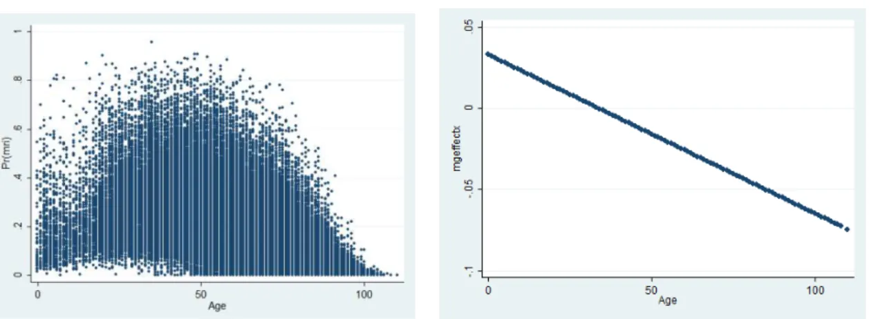
The patient’s age has an interesting pattern of behaviour.

Its impact on the

probability of being sent for an MRI is positive up to a certain threshold, exhibiting

decreasing marginal returns. After that point, we have that the impact of age on the

probability of an individual being sent for MRI is negative. By plotting the patient’s age

and predicted values of

one can observe an inverted-U relationship with an

inflection point around 33 years old

8

. The exact impact of this variable on the

probability of being subject to an MRI depends on the individual’s age –

it is associated

with an expected drop of 0,035

percentage points evaluated at 69,816, the mean of age.

The fact that the patient is female is associated with lower probability of being

sent for an MRI, pointing to the existence of gender discrimination regarding MRI use.

9

As far as the interaction term is concerned, its coefficient tells us how the impact of age

varies according to gender. We have that the interaction term between gender and age

8

This coincides with the domain of the ages of patients being sent for MRI, which ranges from 0 to 104. 9

See Perelman, Mateus and Fernandes (2010) for more on gender differences. They study the case of cardiac heart disease in Portugal and conclude that there is evidence of such discrimination favouring men, especially either prior to acute disease detection or in the case of emergency episodes.

Graphic 1: Scatterplot of individual's age and

(15)

14 bears a positive coefficient. Since the direction of the marginal impact of age varies

depending on the value taken by the regressor, it is useful to look at the effect evaluated

at the mean. That is, at the mean, the marginal effect associated with age is negative, so

we have that its magnitude is lower if the patient is female. In case we are at a point

where the marginal effect of age is positive, then being a female is associated with a

probability of being sent for an MRI that is higher than that for males.

The mortality rate of the corresponding DRG, for the hospital where the patient

was treated, during the three months previous to his release date is also associated with

a drop on the probability of being sent for an MRI as its coefficient bears a negative

sign. The impact of the

severity of the patient’s condition

, in turn, plays an ambiguous

role in explaining the probability of being sent for MRI. In fact, the effects of one extra

procedure and diagnosis on the probability of MRI use go in opposite directions: the

former is associated with an increase whereas the latter has a negative impact. This

result suggests that what matters for the decision on whether to send a patient for MRI

is not how many diagnoses he is made, but rather which diagnoses he is made.

Regarding the time variables, there is evidence of a tightening effect on the

budget constraint of the hospital as all the monthly dummies bear a positive coefficient.

Therefore, one can conclude that a patient admitted in any month from January to

November has a higher probability of being sent for an MRI scan than a similar patient

that is admitted in December, other things equal. Hence, we have a difference in

procedures that is actually reflecting an inefficiency as it cannot be explained by

individual-specific characteristics but rather depends on the time of the year the patient

enters the hospital. Additionally, there seems to be an overtime decreasing trend on the

(16)

15 both these patterns of behaviour vary with the type of hospital that is being considered.

The following table summarizes the results per type of hospital.

10

Table 3: Time variables per type of hospital

Hospital

Overtime trend Tightening of budget constraint

All

Negative

Yes

Central

Positive

Yes

District

Not significant

Yes, though not always significant

Level 1

Positive

Not significant

For the hospital specific variables, we have that an individual being treated in

hospital which is either an EPE or part of a hospital centre has a lower probability of

being sent for MRI than a patient who receives treatment at a hospital which is either an

SPA or does not belong to a hospital centre. Likewise, being treated in a hospital which

celebrated a contract with the Ministry of Health is associated with a probability of

being sent for MRI that is lower than the one of a similar patient treated in a hospital

that did not celebrate such contract.

The size of the hospital is positively associated with the probability of MRI use

as the coefficient associated with the number of patients admitted during the year bears

a positive sign. Conversely, receiving treatment either at a district hospital or a level 1

hospital is associated with a lower probability of MRI use than in the case of central

hospitals. This reinforces the idea that the size of the hospital plays an important role as

hospitals classified as central hospitals are larger than the others. The fact that the

hospital is a teaching hospital exerts a negative impact on the probability of being sent

for MRI, compared to those which are not teaching hospitals.

Now focusing on the determinants of health care demand, there is evidence on

the fact that the probability of an individual being sent for MRI is higher in regions

where average income is higher. The percentage of people above 65, in turn, bears a

10

(17)

16 negative sign suggesting that regions with higher percentage of elderly people tend to

use less technology. Education has an interesting effect as a larger percentage of high

school graduates is associated with a greater probability of MRI use. However, the

higher the percentage of college graduates, the lower the probability of MRI use.

It is worth to develop further on the mechanism trough which these region

specific variables affect the probability of an individual being sent for MRI as adoption

plays a central role in it. The reasoning goes like this: take a hospital located in a low

average income region; most likely, its expectations regarding demand for health care in

general and for hi-tech health care devices in particular are much lower than those of a

hospital located in a wealthier region because wealthier people demand more health

care. Hence, anticipating this lower demand, the hospital is likely to buy less (or even

do not buy at all) MRI equipment since it may feel that the large investment is not worth

it. As a consequence, other things equal, individuals living in regions with lower

average income are less likely to be sent for MRI because there are less scans. An

analogous thinking applies to the remaining region-specific variables.

The coefficients of the urbanization variables suggest that the probability of MRI

use is lower in more urbanized areas as the overall effect of the urbanization variables at

the mean is negative. This result is similar to that obtained in Baker (2001).

Including the hospital fixed effects in the model is a way of considering

differences in clinical practice and hospital preferences regarding technology adoption.

In order to account for the hospital fixed effects in the model, we introduce 80 dummies

(18)

17 correspond to 80 of the 81 hospitals in the sample.

11

This model uses fewer observations

as those referring to hospitals P12, P32, P46, P55, P63 and P65 are automatically

dropped by Stata on the grounds that they predict failure perfectly. P69 is also omitted

because of collinearity. Results are presented in column (2) of table 1.

The pseudo-R

2

of this model is 19, 28%, above that obtained by omitting the

fixed-effects, meaning that hospital characteristics do matter when it comes to predict

the probability of MRI use. This is probably due to differences in the adoption rule

across hospitals. The results are somehow different from those of the previous

specification. While the impact of individual-specific variables is very similar to the

previous one, the time, hospital- and region-specific variables suffered some changes. In

the former case,

there is still evidence of a tightening effect on the hospital’s budget

constraint, but the overtime trend of MRI utilization becomes positive. In the case of the

hospital-specific variables, we have that being an EPE hospital has now a positive effect

on the probability of an individual being sent for MRI. Both the variables corresponding

to the hospital where the patient is treated being part of a hospital centre and to hospital

size keep exerting similar impacts on the probability of MRI use. The remaining

hospital variables lose their significance. As for the region-specific variables, both the

number of physicians and the percentage of high school graduates in the region are

associated with a lower probability of the patient being sent for an MRI scan. Regarding

the variables capturing the degree of urbanization, the number of inhabitants living in

the region still exerts a negative impact when evaluated at its mean, but population

density now contributes towards a higher probability of MRI use. The remaining

variables contained in this vector become statistically undistinguishable from zero.

11

(19)

18 We also address the question of whether patients who were transferred from

another hospital to the current one have a higher probability of being sent for MRI.

Overall, we conclude that the reason why these patients are transferred is more likely to

be linked to the fact that the chances of having access to an MRI scan in the hospital of

origin were low

12

, rather than with more severe medical conditions.

13

At this point we replace the time variables that have been used throughout the

analysis by interactions between the admission year and the admission month

–

i.e.

binary variable that equals one if the patient is admitted in January 2010 and zero

otherwise. This allows every admission month to have a different impact on the

probability that the individual is sent for an MRI depending on the admission year,

whereas before the impact was the same regardless of whether the patient was admitted

at the hospital in January 2008 and in January 2010.

Therefore, the initial model is estimated again, now including these new

time-specific variables rather than the old ones. Eleven equations are estimated: one

including all DRGs and ten others including only one DRG - it may be that the effects

on the probability of an individual being sent for an MRI scan vary across DRGs and

such possibility was disregarded in the previous analysis. A constant is included and

January 2006 is set as benchmark. Additional variables are included when necessary in

order to account for seasonality effects such as the fall in the number of patients sent for

MRI during the summer months. The hospital fixed-effects are disregarded from now

on. The results are discussed in the following lines and presented in the appendix.

12

Note that here what is important is not whether the hospital has MRI equipment or not. Since the MRI scan can be made out of the hospital, what matters is the access that patients have to the examination. 13

(20)

19

-0,3 -0,2 -0,1 0 0,1 0,2 0,3 Fe b May Au g N o v Fe b Ma y Au g N o v Fe b Ma y Au g N o v Fe b Ma y Au g N o v Fe b Ma y

Aug No

v

2006 2007 2008 2009 2010

Coefficient 95% Confidence Interval

As for the model considering the ten DRGs altogether, the sign of the

coefficients bear by individual, hospital and region-specific variables, remains

unchanged relatively to the first model specification.

The analysis of the results of the ten probit models regarding each DRG

individually is not going to be exhaustive. A brief comparison with those obtained for

the whole dataset follows. As far as the significance of the coefficients is concerned, we

have that several variables are no longer statistically distinguishable from zero. Among

those that more often lose their significant are the interaction term between gender and

age, the binary variable capturing the celebration of a contract with the Ministry of

Health and variables such as population density and population squared. Conversely, the

number of physicians in the region gains statistical significance in eight of the ten cases,

though its sign varies depending on the DRG that is considered. Regarding both the sign

and magnitude of the marginal effects, the vast majority of the effects previously found

continues to show up.

Particular emphasis is to be put on the negative coefficients of the new time

variables. Indeed, one can associate them with specific events affecting the economic

and social spheres, which can be linked with the Health sector and affect the use of MRI

technology. The graph below depicts the coefficients associated with the time variables

for the regression including all the DRGs.

(21)

20 First, we highlight the curious pattern of evolution of the series depicted above:

2007 and 2008 are very similar to each other, presenting a relatively flat trend; in the

end of 2008 there is a clear negative jump in the series and from that point on there

seems to be a slightly negative trend along the years of 2009 and 2010 (note that, again,

these two years are very similar to each other).

The bold dots represent the months whose probit coefficients are both negative

and statistically significant: January, April and June, 2009; January, February, May and

June, 2010 and the period ranging from September to December, 2010.

The negative coefficient associated with January 2009 may be linked with the

Supplementary General Budget and the revision of the Stability and Growth Program

which took place during that month. The negative sign corresponding to January and

February 2010 can be linked with the General Budget that was approved in January and

included the usual measures aimed at containing public expenditure in the Health sector.

The period ranging from May to June 2010, in turn, follows the implementation of a

plan developed by the Ministry of Health that was specifically aimed at reducing

expenditure in Portuguese hospitals, which started in late May. As for the final months

of 2010, they follow the announcement of the 3

rd

Stability and Growth Program, which

occurred on the 29

th

of September of that year.

14

As for the remaining bold dots, we could not find any relevant event occurring at

the time that could affect technology use by Portuguese hospitals. Nevertheless, one

recognizes that the effects of the austerity measures mentioned in the previous

paragraphs are in the right direction as a decrease on the probability of a given

individual being sent for MRI is reflected in a fall in overall MRI costs. However, it

14

(22)

21

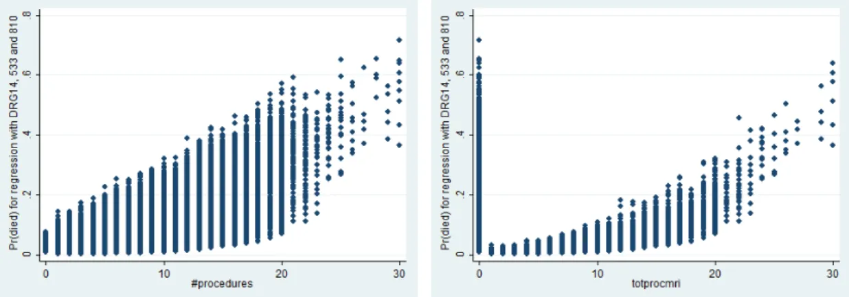
Graphic 5: Scatterplot of number of procedures and predicted values of the probability of death for patients belonging to the 3 DRGs, who were sent for MRI.

seems that the effect of the austerity measures fades away too rapidly, highlighting the

fact that if the Government wants to limit the public expenditure with the Health sector,

then it should opt for a structural reform rather than short term measures.

8. MRI effect on patients’ survival

Finally, we test whether being sent for an MRI does have a positive impact on

the pati

ent’s probability of survival. We

take DRGs 14, 533 and 810, which are those

whose patients more often die and estimate the following probit model.

(

) ( )

, where the dependent variable takes value one if the patient died and zero otherwise.

The independent variables are a binary variable equaling one if the patient was sent for

an MRI and zero otherwise and two vectors containing the previous individual and

hospital variables. Two variables are added to the former vector, which are interactions

between the two measures of illness severity and the fact that a patient is sent for MRI.

We run four probit models, one for each DRG and another one gathering all the

three DRGs. For mean values of both measures of illness severity, being sent for an

MRI does help patients’ survival as the total impact of being sent for

such examination

on the probability of death is negative. This occurs in each of the four regressions.

(23)

22 The new interaction terms allow us to determine where the main gains in

survival come from. Indeed, comparing graphs 3 and 4, one observes that the main

gains from an MRI scan occur mainly for the less severe cases. The scatterplots for the

other interaction term have a similar shape.

The above scatterplots also convey the fact that a high percentage of the most

severe patients is already being sent for MRI

–

4 out of 5 patients who were subject to

29 procedures were sent for the scan. However, those who experience the higher gains

from the examination are those suffering from less severe conditions. Thus, in case of a

contraction on the budget constraint of a hospital, priority should be given to less severe

patients rather than to more severe ones as the former are those who benefit more from

the scan. Conversely, in case of patients suffering from very severe conditions

(particularly those who are made a large number of diagnoses) being sent for an MRI

does not

improve patients’ survival

–

this is can be due to an incomplete control of

illness severity. Such result seems counterintuitive but comes clear-cut from the total

effect of a discrete change of

from 0 to 1 on the probability of death, which

depends on severity of the patient’s condition

: the coefficient associated with the

interaction term of

with the number of diagnoses the patients is made bears a

positive sign and its absolute value exceeds that of the interaction term associated with

the number of procedures. In this sense, patients suffering from more severe conditions

are probably too ill to benefit from the examination.

Note that one cannot state that an MRI exerts a negative impact on survival as it

is no more than a diagnosis tool. Moreover, patients yield benefits from the scanning,

(24)

23 analysis as these could not be measured properly. If total benefits instead of benefits in

terms of probability of death were considered, then conclusions could be altered.

9. Conclusions

This project intends to clarify on the determinants of MRI use for patients with

specific medical conditions, who were admitted at Portuguese NHS hospitals during the

period ranging from 2006 to 2010.

Overall, individual variables are found to be very good predictors of MRI use, as

expected. Indeed, not only their coefficients are very significant, but also their

magnitude is independent of model specification. Variables capturing hospital

characteristics also play a role, though many lose their significance when hospital

fixed-effects are considered in the model specification. As for region-specific variables, one

can say that hospitals seem to account for the characteristics of the regions where they

are located when deciding on their adoption patterns.

There is evidence of a tightening effect on the hospital budget constraint in the

end of the year. This inefficiency suggests that the management of the hospital budget

can be improved. An option to be considered would be not sending for MRI less severe

cases occurring in the beginning of the year as a means to save resources for more

severe cases taking place in the end of the year. Whether correcting this inefficiency

will lead to savings is not clear as the number of patients sent for an MRI scan would

most likely not fall. Nevertheless, it would certainly increase patient’s welfare. Indeed,

the total benefits from sending to an MRI a patient who is in a very severe condition are

likely to be higher than the costs of not sending someone whose condition is not that

(25)

24 year instead of less severe ones occurring in the beginning of the year can be seen as

socially desirable according to the Kaldor-Hicks compensation criteria.

MRI scans are found to help patients’

survival, mainly for those suffering from

less severe conditions. In the case of patients suffering from more severe conditions, the

benefits from an MRI scan in terms of probability of survival are dominated by illness

severity. Nevertheless, this result is not to be taken too far as there are other benefits

from the MRI scan rather than those related to the probability of death. On top of this,

the fact that illness severity is also being poorly measured by the total number of

procedures and diagnoses is likely to have contributed to the result. Still, if one only

cares about patients’ probability of death, then a

policy implication can be drawn: in

case of a fall on the resources available to a given hospital, priority should be given to

less severe cases as these are those who benefit the most from an MRI - the examination

is likely not to yield any significant benefits as far as the probability of death of patients

suffering from more severe conditions is concerned. By adopting this policy we are

improving welfare. Indeed, patients in more severe conditions do not significantly

benefit from the scan, whereas those suffering from less severe conditions do benefit

from it

–

this is a Pareto move as it allows patients in less severe conditions to be better

off without harming those in worse medical conditions (their welfare remains constant).

Note that, again, the number of MRIs most likely will not fall. The only change is that

the patients being sent for the examination are in a better medical condition.

All in all, given the nature of the inefficiencies found in the use of MRI across

Portuguese NHS hospitals for patients suffering from specific conditions, it is not clear

whether correcting them would allow for cost reductions. Still, there is definitely room

(26)

25

10. References

Baicker, Katherine and Amitabh Chandra.

2011. “Aspirin, Angioplasty and Proton

Beam Therapy: The Economics of Smarter Health Care Spending.”

http://www.kc.frb.org/publicat/sympos/2011/2011.BaickerandChandra.paper.pdf.

Baker, Laurence.

2001. “Managed care and technology adoption in health care:

Evidence from Magnetic Resonance Imaging.”

Journal of Health Economics, 20:

395-421.

Barros, Pedro Pita, and Xavier Martinez-Giralt.

2009

. “Technolo

gical adoption in

health care.”

http://digital.csic.es/bitstream/10261/35483/1/79009.pdf.

Cameron, A. Colin and Pravin K. Trivedi.

2009. “Binary Outcome Models.” In

Microeconometrics, 8

th

edition, 463-474. New York: Cambridge University Press.

Chandra, Amitabh and Jonathan S. Skinner.

2011. “Technology Growth and

Expenditure in Health Sector.”

NBER Working Paper 16953.

Congressional Budget Office.

January 2008, Technological Change and the Growth of

Health Care Spending.

Dengler, Philipp Schmidt-.

2006. “The timing of new technology adoption: the case of

MRI.”

http://personal.lse.ac.uk/schmidt1/mri_june.pdf.

Hillman, Alan and J. Sanford Schwartz.

1986. “The diffusion of MRI: Patterns of

siting and ownership in an era of changing incentives.”

American Journal of

Roentgenology, 142: 963-969.

Kung, Pei-Tseng, Wen-Chen Tsai, Chih-Liang Yaung and Kai-Ping Liao.

2005.

“Determinants of computed tomography and magnetic resonance imaging utilization in

Taiwan.”

International Journal of Technology Assessment in Health Care, 21(1): 1-8.

Oh, Eun-Hwan, Yuichi Imanaka, and Edward Evans.

2005. “Determinants of the

diffusion of computed tomography and magnetic imaging.”

International Journal of

Technology Assessment in Health Care, 21(1): 73-80.

Perelman, Julian, Céu Mateus and Ana Fernandes.

2010. “

Gender equity in

treatment for cardiac heart disease in Portugal

.”

Social Science & Medicine, 71(1):

25-29.

Teplensky, Jill D., Mark V. Pauly, John R. Kimberly, Alan L. Hillman and J.

Sanford Schwartz

. 1995. “Hospital adoption of medical technology: An empirical test

(27)

THE USE OF TECHNOLOGY IN PORTUGUESE HOSPITALS

–

THE CASE OF MRI - APPENDICES

ANA CLÁUDIA DIAS MENDES CORREIA MOURA

STUDENT NUMBER 414

A Project carried out in the Applied Policy Economics area, under the supervision of:

Professor Pedro Pita Barros

(28)

(29)

2 analysis, one finds evidence of a negative overtime trend of MRI use as well as a

tightening effect on the hospital’s budget constraint taking place in December. In this

section, I look deeper at this pattern of behavior and check whether it differs with the

type of hospital: central, district and level 1.

In fact, for the case of central hospitals, there is still evidence of a tightening

effect on the hospital’s budget constraint, but the sign of the o

vertime trend on MRI use

is positive. Regarding district hospitals, there is evidence of the tightening effect,

though not for all the months as some of them lost their significance. The coefficient

that yields the overtime trend also becomes non-significant. Finally, level 1 hospitals

exhibit a positive overtime trend on the use of MRI scans and show no evidence of a

tightening effect on their budget constraints.

a)

For central hospitals:

Probit regression Number of obs = 86103 LR chi2(34) = 12630.56 Prob > chi2 = 0.0000 Log likelihood = -32736.632 Pseudo R2 = 0.1617

(30)

3

hcenter | -.0506056 .0284304 -1.78 0.075 -.1063282 .0051169 contract | -.1905186 .0248991 -7.65 0.000 -.23932 -.1417172 totinterns | .008565 .0003711 23.08 0.000 .0078376 .0092923 distrital | -.7213586 .0626243 -11.52 0.000 -.8441001 -.5986172 nivel1 | (omitted)

ensino | -.3208708 .03205 -10.01 0.000 -.3836876 -.2580541 income | .0009631 .0006078 1.58 0.113 -.0002281 .0021544 elderly | -.0577392 .0914599 -0.63 0.528 -.2369974 .121519 physicians | .0079909 .0243632 0.33 0.743 -.03976 .0557419 hschool | -.0429995 .0110224 -3.90 0.000 -.0646029 -.021396 college | -.0544654 .0240155 -2.27 0.023 -.1015348 -.0073959 pop | .8209526 .2872198 2.86 0.004 .2580122 1.383893 pop2 | -.0214527 .0077149 -2.78 0.005 -.0365737 -.0063317 dpop | -4.388516 4.815025 -0.91 0.362 -13.82579 5.048759 dpop2 | .0006261 .0020337 0.31 0.758 -.0033598 .0046121 _cons | -110.7944 35.62393 -3.11 0.002 -180.616 -40.97274

b)

For district hospitals:

--- mri | Coef. Std. Err. z P>|z| [95% Conf. Interval] ---+--- gender | -.516586 .0453082 -11.40 0.000 -.6053884 -.4277835 age | .0317086 .0019238 16.48 0.000 .027938 .0354792 age2 | -.0004885 .0000159 -30.69 0.000 -.0005197 -.0004573 genderage | .0071496 .000672 10.64 0.000 .0058326 .0084667 totproc | .1081159 .0021415 50.48 0.000 .1039186 .1123133 totdiag | -.0578624 .0029748 -19.45 0.000 -.0636928 -.052032 mrate | -3.112418 .1724115 -18.05 0.000 -3.450338 -2.774498 year | -.0071624 .0050189 -1.43 0.154 -.0169993 .0026745 adjan | -.0044052 .0252042 -0.17 0.861 -.0538046 .0449942 adfeb | .0293076 .025831 1.13 0.257 -.0213203 .0799354 admar | .0477923 .0251426 1.90 0.057 -.0014864 .097071 adapr | .0519402 .0207675 2.50 0.012 .0112366 .0926438 admay | .0594043 .0265083 2.24 0.025 .0074491 .1113596 adjun | .0305324 .0270678 1.13 0.259 -.0225196 .0835844 adjul | .0674495 .0265822 2.54 0.011 .0153494 .1195497 adaug | .0343651 .0269694 1.27 0.203 -.018494 .0872241 adsep | .0708732 .0269677 2.63 0.009 .0180174 .1237289 adoct | .0925414 .0263104 3.52 0.000 .040974 .1441089 adnov | .070316 .0266292 2.64 0.008 .0181238 .1225082 epe | .029332 .0180565 1.62 0.104 -.0060582 .0647222 hcenter | -.1328612 .0152915 -8.69 0.000 -.162832 -.1028904 contract | .0181658 .0255307 0.71 0.477 -.0318734 .068205 totinterns | .0128394 .0006179 20.78 0.000 .0116284 .0140505 distrital | (omitted)

nivel1 | (omitted)

(31)

4

Log likelihood = -1059.2357 Pseudo R2 = 0.2041

--- mri | Coef. Std. Err. z P>|z| [95% Conf. Interval] ---+--- gender | -1.019932 .2783452 -3.66 0.000 -1.565478 -.4743852 age | .0039634 .011871 0.33 0.738 -.0193034 .0272301 age2 | -.0003241 .0000937 -3.46 0.001 -.0005077 -.0001404 genderage | .014501 .0039685 3.65 0.000 .0067229 .0222791 totproc | .141077 .0110814 12.73 0.000 .1193579 .1627962 totdiag | -.0730495 .0154794 -4.72 0.000 -.1033885 -.0427104 mrate | -.4752486 .3616484 -1.31 0.189 -1.184066 .2335693 year | .2834349 .0456386 6.21 0.000 .1939849 .3728849 adjan | .0970396 .1224182 0.79 0.428 -.1428956 .3369748 adfeb | .1171819 .1272977 0.92 0.357 -.132317 .3666807 admar | .1487235 .1230027 1.21 0.227 -.0923574 .3898044 adapr | .0886665 .0985699 0.90 0.368 -.1045268 .2818599 admay | .0974091 .1348154 0.72 0.470 -.1668242 .3616423 adjun | .1514557 .1362668 1.11 0.266 -.1156222 .4185336 adjul | .0591196 .1378887 0.43 0.668 -.2111373 .3293764 adaug | -.0297607 .1439081 -0.21 0.836 -.3118155 .252294 adsep | .0482225 .1422212 0.34 0.735 -.2305261 .326971 adoct | .1552915 .1347659 1.15 0.249 -.1088448 .4194279 adnov | .1690035 .1356304 1.25 0.213 -.0968271 .4348341 epe | -.2822461 .2269928 -1.24 0.214 -.7271439 .1626516 hcenter | .0067172 .1103334 0.06 0.951 -.2095323 .2229667 contract | .2459139 .4299667 0.57 0.567 -.5968055 1.088633 totinterns | .0557567 .0206431 2.70 0.007 .015297 .0962165 distrital | (omitted)

nivel1 | (omitted) ensino | (omitted)

income | -.0089733 .0031958 -2.81 0.005 -.0152369 -.0027097 elderly | .2074338 .0513005 4.04 0.000 .1068866 .3079811 physicians | .0613139 .0980986 0.63 0.532 -.1309557 .2535836 hschool | -.1256668 .0490991 -2.56 0.010 -.2218994 -.0294343 college | .0867352 .0616306 1.41 0.159 -.0340586 .207529 pop | -.2145631 .1591718 -1.35 0.178 -.5265341 .0974079 pop2 | .0919869 .0209822 4.38 0.000 .0508626 .1331113 dpop | 3.000871 1.702882 1.76 0.078 -.3367161 6.338459 dpop2 | -.0067146 .0013389 -5.01 0.000 -.0093389 -.0040903 _cons | -566.7172 91.03508 -6.23 0.000 -745.1427 -388.2917

3. Transferred patients

(32)

5 average. Hence, the reason why these patients are transferred is more likely to be linked

to the fact that the chances of

having access to an MRI scan in the hospital of origin

were low

1

, rather than with more severe medical conditions

–

one expects patients to be

independently and identically distributed across hospitals, so that the probability that a

more severe one shows up is the same across hospitals. This variable is disregarded in

the main analysis as it implies a large loss of observations.

The regression table relative to this analysis is presented below.

adjan | .1315498 .0493884 2.66 0.008 .0347504 .2283491 adfeb | .0947136 .051102 1.85 0.064 -.0054445 .1948717 admar | .1173838 .0497736 2.36 0.018 .0198293 .2149384 adapr | .1036135 .0510928 2.03 0.043 .0034735 .2037535 admay | .1104024 .0504682 2.19 0.029 .0114865 .2093182 adjun | .1413863 .0506874 2.79 0.005 .0420407 .2407318 adjul | .1627495 .050729 3.21 0.001 .0633224 .2621765 adaug | .1985464 .0506997 3.92 0.000 .0991768 .297916 adsep | .1628059 .0507174 3.21 0.001 .0634016 .2622101 adoct | .1548554 .0502388 3.08 0.002 .0563892 .2533216 adnov | .1262391 .0507543 2.49 0.013 .0267625 .2257158 epe | -.2467363 .0254775 -9.68 0.000 -.2966713 -.1968014 hcenter | .2945691 .0264213 11.15 0.000 .2427843 .346354 contract | -.2809066 .0432739 -6.49 0.000 -.3657219 -.1960914 totinterns | .0145707 .0013121 11.11 0.000 .0119991 .0171423 distrital | -.1086734 .0314198 -3.46 0.001 -.170255 -.0470918 nivel1 | -.6715543 .06978 -9.62 0.000 -.8083206 -.5347881 ensino | -.0870849 .0381078 -2.29 0.022 -.1617748 -.0123951 income | .0090671 .0012158 7.46 0.000 .0066843 .01145 elderly | .0555203 .0121819 4.56 0.000 .0316442 .0793964 physicians | -.0286771 .0067171 -4.27 0.000 -.0418423 -.0155118 hschool | -.0010876 .0275972 -0.04 0.969 -.0551771 .053002 college | -.2326342 .0255964 -9.09 0.000 -.2828023 -.1824662 pop | -.0980163 .0340619 -2.88 0.004 -.1647765 -.0312561 pop2 | .0014872 .000875 1.70 0.089 -.0002278 .0032021 dpop | 3.914751 .3902852 10.03 0.000 3.149806 4.679696 dpop2 | -.0017519 .0002333 -7.51 0.000 -.0022092 -.0012947 transferido | .0510356 .0261801 1.95 0.051 -.0002764 .1023477

1

(33)

6 admission month

The eleven regression tables for these regressions are presented below. The

coefficients for the interactions between the admission year and the admission month

that are statistically significant and bear a negative sign are highlighted in red.

a)

For all the DRGs together:

(34)

7

apr2008 | .0583151 .0420763 1.39 0.166 -.024153 .1407832 may2008 | .0996629 .0419898 2.37 0.018 .0173644 .1819615 jun2008 | .063416 .0428379 1.48 0.139 -.0205447 .1473766 jul2008 | .0723648 .0416856 1.74 0.083 -.0093374 .1540671 aug2008 | .1053245 .0421832 2.50 0.013 .022647 .1880021 sep2008 | .0831625 .0419927 1.98 0.048 .0008583 .1654667 oct2008 | .1431187 .0406529 3.52 0.000 .0634405 .2227968 nov2008 | .0673401 .0412256 1.63 0.102 -.0134607 .1481408 dec2008 | -.0170116 .0423676 -0.40 0.688 -.1000507 .0660274

feb2009 | -.0375333 .0427529 -0.88 0.380 -.1213273 .0462608 mar2009 | -.0379001 .0413885 -0.92 0.360 -.1190201 .0432199

may2009 | -.0542474 .042267 -1.28 0.199 -.1370891 .0285944

jul2009 | .0157551 .041343 0.38 0.703 -.0652757 .0967859 aug2009 | -.0293666 .0418559 -0.70 0.483 -.1114027 .0526696 sep2009 | .0009829 .0415533 0.02 0.981 -.08046 .0824258 oct2009 | -.024499 .0415038 -0.59 0.555 -.105845 .0568469 nov2009 | -.0244977 .0411288 -0.60 0.551 -.1051087 .0561132 dec2009 | -.046943 .0413121 -1.14 0.256 -.1279133 .0340273

mar2010 | -.0478459 .0409935 -1.17 0.243 -.1281916 .0324998 apr2010 | -.0627723 .0417501 -1.50 0.133 -.1446009 .0190564

aug2010 | -.0580922 .0422829 -1.37 0.169 -.1409653 .0247808

_cons | -2.902781 .1388553 -20.91 0.000 -3.174933 -2.63063

b)

For DRG533: