CALCULATION OF PARAMETER RANGES FOR ROBUST GAIN TUNING
OF POWER SYSTEM CONTROLLERS
Ricardo Vasques de Oliveira
∗Rodrigo Andrade Ramos
†Newton Geraldo Bretas
†∗Departamento de Engenharia Elétrica - Universidade Tecnológica Federal do Paraná,
Via do Conhecimento, Km 1, 85503-390, Pato Branco, PR, Brasil.
†Departamento de Engenharia Elétrica - Escola de Engenharia de São Carlos - USP
Av. Trabalhador São-carlense, 400, 13566-590, São Carlos, SP, Brasil.
RESUMO
Cálculo de Faixas de Parâmetro para o Ajuste Robusto do Ganho de Controladores de Sistemas de Potência O presente trabalho propõe uma ferramenta computacional para auxiliar engenheiros de sistemas de potência no ajuste em campo de controladores de amortecimento e reguladores automáticos de tensão. A abordagem proposta gera faixas de valores de parâmetros para o ajuste em campo dos controla-dores do sistema. As faixas de valores geradas teoricamente garantem a estabilidade para o sistema em malha fechada. Estas faixas de valores são dadas na forma de valores limites para os ganhos estáticos dos controladores de interesse, de maneira que o engenheiro responsável pelo ajuste em campo dos controladores tenha garantia da estabilidade do sistema durante o ajuste do ganho do controlador. Esta característica da abordagem proposta é altamente desejavel do ponto de vista prático, pois a etapa de comissionamento de controla-dores de amortecimento e regulacontrola-dores automáticos de tensão sempre envolve algum reajuste dos ganhos dos controlares, devido às diferenças entre o modelo nominal e o comporta-mento real do sistema. Considerando essas diferenças como incertezas no modelo, a ferramenta proposta é capaz de ga-rantir estabilidade para o modelo incerto usando uma abor-dagem baseada em desigualdades matriciais lineares. A
me-Artigo submetido em 26/01/2011 (Id.: 1257) Revisado em 15/07/2011, 28/09/2011
Aceito sob recomendação do Editor Associado Prof. Takashi Yoneyama
todologia proposta pode ser também aplicada para o ajuste de outros tipos de parâmetros de controladores de amorte-cimento, assim como para o ajuste de outros tipos de con-troladores (por exemplo, reguladores de velocidade). Dois modelos de sistemas de potência tipicamente utilizados em estudos de estabilidade são considerados para a aplicação e avaliação da ferramenta proposta.
PALAVRAS-CHAVE: Dinâmica e controle de sistemas de po-tência, estabilidade a pequenas perturbações, estabilizador de sistemas de potência, regulador automático de tensão, con-trole robusto, desigualdade matricial linear.
ABSTRACT
and AVR commissioning stage always involve some read-justment of the controller gains to account for the differences between the nominal model and the actual behavior of the system. By capturing these differences as uncertainties in the model, this computational tool is able to guarantee stabil-ity for the whole uncertain model using an approach based on linear matrix inequalities. It is also important to remark that the tool proposed in this paper can also be applied to other types of parameters of either PSSs or Power Oscilla-tion Dampers, as well as other types of controllers (such as speed governors, for example). To show its effectiveness, ap-plications of the proposed tool to two benchmarks for small signal stability studies are presented at the end of this paper.
KEYWORDS: Power system dynamics and control, small signal stability, power system stabilizer, automatic voltage regulator, robust control, linear matrix inequality.
1
INTRODUCTION
The reliability and performance of power systems, in tran-sient and steady-state conditions, strongly depend on the de-sign and field tuning of the system controllers (stabilizers, automatic voltage regulators, speed governors, and so on). In most cases, power system controllers, even when designed by methodologies that ensure some level of robustness with respect to variations of the system operating conditions, re-quire additional tuning during the commissioning stage in or-der to provide an acceptable performance for the closed loop power system. This retuning may be necessary, for example, due to normal changes in the operating conditions of the sys-tem. The topology and the typical daily load curve of power systems may naturally change along the time, which lead to the need for a field retuning of the controllers.
The need for the treatment of the mentioned power sys-tem characteristics has lead to the development of many ap-proaches for the design and tuning of PSSs and damping con-trollers (Bomfim et al., 2000; Zanchin and Bazanella, 2003; Abdel-Magid and Abido, 2003; Zanetta and Cruz, 2005; Cai and Erlich, 2005; de Oliveira et al., 2010a; Gurrala and Sen, 2010; Jabr et al., 2010; Furini et al., 2011). However, most design and tuning procedures based on robust control techniques proposed up to now do not consider the need of a field retuning of the designed controllers.
It is worth mentioning that the engineer who carries out the controller (PSS, AVR, and so on) retuning in field tests is not usually the same engineer who designed it. In this way, the engineer responsible for the controller retuning may not know the theoretical limits within which the controller pa-rameters can be changed to ensure the desired small-signal stability margin for the system. Furthermore, the commis-sioning of power system controllers is typically an
empiri-cal procedure which consists in introducing small changes in the static gain of the controller and carefully monitoring the power station dynamics in the control room until an accept-able response is obtained.
In this context, this work proposes a tool to assist power system engineers in retuning and/or commissioning of PSSs and/or AVRs. This tool provides theoretical limits for the en-gineer to carry out a safe field retuning, thus avoiding that the new gain settings threaten the power system reliability and stability. Using these theoretical limits, a range of values is provided, in such a way that any value within this range can be used in the retuning of the controller static gain, result-ing in guaranteed closed loop stability from the theoretical viewpoint. It is also important to remark that a certain small-signal stability margin may be the chosen criterion for which a theoretical guarantee must be sought, and this is indeed the approach used in this paper, to comply with the typical prac-tice in power system stabilizer design and assessment. This guarantee is obtained using a formulation based on linear ma-trix inequalities (LMIs).
The methodologies for the tuning of PSS usually supply fixed values for the parameters to be tuned. Abdel-Magid and Abido (2003), Cai and Erlich (2005), and Jabr et al. (2010), for example, have presented procedures to determine fixed values for the parameters of the PSS to be tuned (i.e., fixed settings for the PSS parameter). Different from the typical tuning approaches, this paper proposes a methodology that provides continuous parameter ranges for the field tuning of PSS. Besides, the approach proposed in this paper is also ap-plicable to AVR and other kinds of power system controllers.
The paper is structured as follows. Section 2 depicts the fundamentals employed in the formulation of the proposed tool and Section 3 presents the computational tool itself. The evaluation of the proposed tool is carried out by applying it to two benchmark test systems in Section 4, and Section 5 presents the conclusions taken from this evaluation and from the overall approach presented in this paper.
2
FUNDAMENTALS OF THE PROPOSED
TOOL
The development of the computational tool proposed in this work was based on the theory of Affine Parameter-Dependent Lyapunov Functions, particularly those that can be put in the form of LMIs (Gahinet et al., 1996; Oliveira and Peres, 2005). This section presents the fundamentals of this development to enable a better comprehension of the overall mechanism of the proposed tool.
˙˜
x=f(˜x,u˜,˜z), (1)
0=g(˜x,u˜,˜z), (2)
˜
y=h(x˜,˜u,˜z), (3)
wherex˙˜∈Rnis the system state vector,u˜∈Rpis the con-trol input vector,˜y∈Rqis the measured output, andz∈Rm is the vector with the algebraic variables. However, when it comes to controller design and small signal stability studies in power systems, models obtained from the linearization of equations (1)-(3) are usually employed.
The equation resulting from the linearization of (2) is typi-cally eliminated by substituting it into the equations resultant from (1) and (3). The resulting linearized model of a power system can be represented by
˙
x=Ax+Bu, (4)
˙
y=Cx+Du. (5)
In (4)-(5),x∈Rncorresponds to the deviation from an equi-librium point˜xeof (1) and (3). In a similar way,u∈Rpand y ∈ Rq represent the deviations from u˜
e and˜ye, respec-tively. Linear controllers for power systems can be repre-sented by models in the form
˙
xc=Acxc+Bcu, (6)
u=Ccxc, (7)
wherexc ∈ Rs is the vector with the controller state vari-ables. The closed-loop model of the controlled power sys-tem, obtained from the connection of (4)-(5) with (6)-(7), considering the controller parameter dependence, can be rep-resented by
˙¯
x=A¯(ρ)¯x, (8)
wherex¯= [x xc]T and
¯
A=
[
A BCc(ρ)
Bc(ρ)C Ac(ρ) +Bc(ρ)DCc(ρ)
]
. (9)
In (8), ρ ∈ Rk is a vector with the controller parameters
to be tuned. The controller parameters are considered to be
time invariant (i.e.,ρ˙ = 0) in this work, given that the static gains of power system controllers are usually fixed after the commissioning stage. MatrixA¯(ρ)is affine parameter-dependent, that is,
¯
A(ρ) =A¯0+A¯1ρ1+· · ·+A¯kρk, (10)
whereA¯0,A¯1,· · ·,A¯kare constant matrices. Since eachρi, fori= 1,· · ·, k,is associated with one of the controllers to be commissioned or retuned, the coefficients of the matrix
¯
Aidescribe the manner in which the i-th parameter affects the dynamics of the whole system.
The developments in this paper are based on the assumption that each parameterρibelongs to a known range defined by its extreme limitsρ
iandρ¯i, that is,
ρi∈[ρiρ¯i], (11)
whereρiis the lower bound andρ¯iis the upper bound for the range of values of parameterρi. Both bounds are specified in advance in order to define an acceptable uncertainty range for the parameter of the controller to be tuned. These specified bounds for the parameter vector describe an hyper-rectangle inRk, whose the vertices are given by
v:={(ρ1,· · ·, ρk) :ρi∈[ρiρ¯i] }
. (12)
A quadratic Lyapunov function for (8) may be written as
V(x¯, ρ) =¯xTP(ρ)¯x, (13)
whereP(ρ)is also an affine function given by
P(ρ) =P0+P1ρ1+· · ·+Pkρk. (14)
Sufficient conditions for stability of (8) can be written in the form of LMIs. Defining
ρavg:= [
1+ ¯ρ1 2 ,· · ·,
k+ ¯ρk
2
]
whereρavgis the average value of the parameter vector, it is possible to state (Gahinet et al., 1996) that the system (8) is affinely quadratically stable ifA¯(ρavg)is stable and
P0+P1ρ1+· · ·+Pkρk ≻0, (16)
¯
A(ρ)TP(ρ) +P(ρ)A¯(ρ) +∑k
i=1ρ 2
iµiI≺0, (17) ¯
ATiPi+PiA¯i+µiI≻0, (18)
for allγ∈ν,µi≻0andi= 1,· · · , k.From (10) and (14), inequality (17) may be rewritten as
¯
AT0P0+P0A¯0
+∑k
i=1ρi(
¯
A0TPi+PiA¯0+A¯TiP0+P0A¯i)
+∑i<j
i>0ρiρj(
¯
AiTPj+PjA¯i+A¯TjPi+PiA¯j)
+∑k
i=1ρ 2
i(A¯Ti Pi+PiA¯i) + ∑k
i=1ρ 2
iµiI≺0, (19)
for i = 1,· · ·, k. It is worth mentioning that the scalarµ
is included in the LMI formulation to reduce control formu-lation conservatism and to avoid numerical problems in the solver employed to resolve the LMIs.
From the controller tuning viewpoint, it is mandatory that the variations in the operating conditions of the system are taken into account. Therefore, to comply with the typical practice
in power systems, a number of linearized models (which can be extracted from the daily load curves, for example) in the form of (8) are employed in the formulation so the changes in the operating conditions are properly addressed.
Taking multiple operating conditions into account, the sys-tem (8) can be rewritten in the form
˙¯
x=A¯j(ρ)x¯, (20)
wherej= 1,· · ·, L,
¯
Aj(ρ) =
[
Aj BjCC(ρ)
BC(ρ)Cj AC(ρ) +BC(ρ)DjCC(ρ)
]
,
(21)
and L is the number of operating conditions considered to generate the parameter range.
Furthermore, the typical practice in small-signal stability analysis and control of power systems dictates that a cer-tain small-signal stability margin must be respected in the overall closed loop system (Gomes et al., 2003), to avoid that eigenvalues with very low damping ratio pose a threat to system stability with respect to variations in the operating conditions. The proposed tool can comply with this practice by means of the regional pole placement technique (Chilali et al., 1999; de Oliveira et al., 2010a). Using this technique, LMIs (16)-(18) are transformed into
P0+P1ρ1+· · ·+Pkρk ≻0, (22)
sinθ(A¯(ρ)T
jP(ρ) +P(ρ)A¯(ρ)j )
cosθ(
P(ρ)A¯(ρ)j−A¯(ρ)T
jP(ρ) )
cosθ(¯
A(ρ)T
jP(ρ)−P(ρ)A¯(ρ)j )T
sinθ(A¯(ρ)T
jP(ρ) +P(ρ)A¯(ρ)j )
+ ∑k
i=1ρ 2
iµiI≺0, (23)
¯
ATijPi+PiA¯ij+µiI≻0, (24)
fori = 1,· · · , kandj = 1,· · ·, L. In (23),θ = cos−1ζ 0,
withζ0 being the minimal damping ratio for the response
modes of all power system models.
If a feasible solution to LMIs (22)-(24) is found, the resulting parameter range ensures that the eigenvalues of all the con-sidered power system models (with the inclusion of the tuned controllers) will present damping ratios higher thanζ0.
3
DESCRIPTION OF THE PROPOSED
COMPUTATIONAL TOOL
Classical phase compensation is the approach usually em-ployed by the industry to design PSSs. The traditional struc-ture of a phase compensator is shown in the block diagram in Fig. 1, with the washout block added to ensure zero gain in steady-state conditions. In Fig. 1, the subscriptidenotes the
In this paper, two lead-lag blocks were used for each retuned PSS, which corresponds to Fig. 1 withnc= 2. In this work,
yicorresponds to the speed deviation of thei-th system gen-erator anduiis thei-th stabilizing signal applied to the ref-erence of the AVR. This stabilizing control loop is a decen-tralized control loop, since it adopts a local measurement.
Figure 1: Block diagram of a typical PSS based on phase compensation.
In order to include such a controller in the formulation (22)-(24) (more specifically in matrixA¯(ρ)j), the block diagram model showed in Fig. 1 was converted to its corresponding state-space model (6)-(7) (Further details about such model conversion may be found in de Oliveira et al. (2010a)).
The AVR has a significant impact on the small signal stability margin of power systems (Kundur, 1994; Machowski et al., 2008; Ramos, 2009). In this way, the tuning of this kind of regulator is quite important for the stability and reliability of power systems. In this study, the AVR is assumed as a first-order regulator, whose block diagram is given in Fig. 2. In this figure, Ke is the AVR static gain, Te is the AVR time constant,EF Dis the voltage applied to the field circuit,Vtis terminal voltage,Vref is the reference voltage for the AVR, anduis the stabilizing signal from the PSS.
Figure 2: Block diagram of the AVR employed in power sys-tem model.
The computational tool proposed in this paper is based on the application of the fundamentals described in the previ-ous section to the problem of generating a range of values for theKpss_iand/orKe_istatic gains to be employed in the commissioning or retuning of the controllers. Theρ param-eter vector, presented in the formulation (22)-(24), is com-posed by the static gains of the controllers (ρi =Kpss_i or
ρi=Ke_i).
These parameters were chosen because some operating con-ditions of power systems demand a retuning of the static gain of PSSs and/or AVRs to improve the system small-signal
sta-bility margin and avoid detrimental sustained oscillations in the operation of the corresponding generators.
As previously mentioned, the range of parameter values gen-erated by the proposed tool ensures that the eigenvalues of each of the considered power system models with the retuned controllers will exhibit damping ratios higher than a pre-specified value (ζ0). To illustrate this feature, Fig. 3 presents
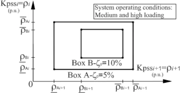
a hypothetical range ofKpssvalues guaranteeing a damping ratio higher than 5% (Range A) for the eigenvalues of power system models in medium and high loading conditions. If a damping ratio higher than 10% is sought for the same condi-tions, usually the corresponding range ofKpssvalues (Range B) will be smaller than the previous one, as also illustrated in Fig. 3 (although this is not a rule, given the nonlinear na-ture of the power system model). According to Fig. 3, any value ofKpss = ρbelonging to the range A ([ρAρ¯A]), for example, provides a PSS tuning which ensures a damping ra-tio higher than 5% for the eigenvalues of the power system models in the adopted loading conditions. The lower and up-per bounds for the parameter range (ρandρ¯, respectively) are generated by the tool proposed in this paper.
Figure 3: Illustrative example of the proposed parameter ranges for hypothetical retuning of a single PSS.
This proposed formulation allows two retuning strategies: the retuning of only one controller gain at a time or the si-multaneous retuning of multiple controller gains. In the for-mer strategy, the parameter range is calculated only for one controller, considering a multimachine system model with all the other controllers unchanged. This is the most common situation, where the controller of a single plant is being com-missioned or retuned while the others are under operation, and is also the situation illustrated in Fig. 3.
criterion for all eigenvalues of each of the considered power system models.
As described in the previous section, these parameter ranges or boxes are calculated by means of an algorithm which in-volves LMIs (22)-(24). Roughly speaking, the algorithm consists in finding a feasible solution to the mentioned LMIs after setting the bounds forρi parameters ([ρi ρ¯i]), choos-ing the system operatchoos-ing points of interest, and definchoos-ing the desired minimum damping ratio for the eigenvalues of all power system models.
The algorithm begins with the choice of the controllers to be tuned, system operating conditions of interest, and desired minimum damping ratio. Given that commissioning or re-tuning of PSS/AVR gains are the problems being addressed in this paper, the nominal values of the parameter to be tuned (Kpss0_i=ρi{o}/Ke0_i=ρi{o}) are given in advance by the
outcome of the PSS/AVR design problem. The limits forρi parameters ([ρiρ¯i]) are determined by means of small param-eter changes (∆ρ) as the algorithm iterates. The algorithm employs positive and negative changes with magnitude∆ρ
with respect to the nominal value of theρiparameter (ρi{o})
in order to determine the new limits of the safe parameter range (ρi{k} =ρi{k−1}−∆ρandρ¯i{k} = ¯ρi{k−1}+ ∆ρ).
The value of∆ρmay be chosen as a percentage of the nom-inal value of theρiparameter.
Figure 4: Illustrative example of the proposed parameter ranges for hypothetical retuning of two PSSs at once.
The algorithm iterates until the solver employed to resolve the LMIs (22)-(24) fails to find a feasible solution to the problem. It is worth mentioning that for the vast majority of LMI solvers available to carry out this algorithm, failure to reach a solution to LMIs (22)-(24) does not necessarily imply the non-existence of a feasible solution for them.
As an empirical strategy to explore the nature of the PSS and AVR retuning problem, in order to search for a wider range of safe parameter values, the algorithm initially ap-plies negative changes with respect to the nominal value of the ρi parameter. After finding a lower bound on the pa-rameter range (ρi{k}), positive changes are applied until the
upper bound of the parameter range (ρ¯i{k}) is found in a
sim-ilar manner. The algorithm searches for the lower bound of the parameter range first due to the practical importance of this bound in the PSS adjustment, since the border between the acceptable and unacceptable small-signal stability mar-gin for the system is usually reached with the lowest accept-able value of the PSS gain. On the other hand, the upper bound of the parameter range is usually chosen with the ob-jective of avoiding saturation of the controller output and un-desired amplification of high-frequency dynamics. Fig. 5 il-lustrates this strategy. This example considers the retuning of only one PSS gain and a desired minimum damping ratio of 10%. In Fig. 5,ρi{0}is the nominal value of the
param-eter (i.e., nominal value of the static gain of the i-th PSS to be tuned), ρ
i{2=lower} is the lower bound of the
gener-ated parameter range,ρ¯i{F inal=upper}is the upper bound of
the generated parameter range. In other words, ρ
i{2=lower}
andρ¯i{F inal=upper}are the lowest and highest values for the
static gain that formally assure a damping ratio of 10% for the response modes of the power system with the tuned con-trollers.
Under the previously stated context, the computational tool for PSS and AVR gain retuning proposed in this paper con-sists in the following algorithm:
Step 1: Choose the controllers to be tuned, the operating conditions of interest, and the minimum damping ratio for the close loop system with the tuned controllers;
Step 2: Initialize the parameter bounds using the nominal value of the parameter (ρi{0}= ¯ρi{0}=ρi{0});
Step 3: Set k:=0 and choose the value of∆ρto be employed in the calculation of the parameter bounds (ρi{k+1}and
¯
ρi{k+1});
Step 4: Set k=k+1 and determine thek-thupdate on the pa-rameter bounds byρi{k}=ρi{k−1}−∆ρandρ¯i{k}=
¯
ρi{k−1} (note that the upper bound is kept constant in
this step);
Step 5: Minimizeµsubject to LMIs (22)-(24);
Step 6: If a feasible solution was found in Step 5, return to Step 4; Otherwise, setρi{k−1}=ρi{f inal_min}; Step 7: Set k=k+1 and determine thek-thparameter bounds
by ρ¯i{k} = ¯ρi{k−1}+ ∆ρandρi{k} = ρi{k−1}(note
that the lower bound is kept constant in this step);
Step 8: Minimizeµsubject to LMIs (22)-(24);
Step 10: Setρ¯i{k−1} = ¯ρi{f inal_max}and stop; The
result-ing range of parameter values to be employed in the commissioning or retuning of the controllers is given by[ρ
i{f inal_min},ρ¯i{f inal_max}].
Figure 5: Illustration of the iterative process employed in the calculation of the range of parameter values.
4
TESTS AND RESULTS
A number of tests have been performed to validate and eval-uate the outcomes of the proposed tool. The tests were carried out based on two power system models which are benchmarks for small signal stability studies (Kundur, 1994; Rogers, 2000). After evaluating the convergence properties of the proposed algorithm, the robustness of the resulting ranges of parameter values with respect to the desired small-signal stability margin were validated by means of linear and non-linear analyses.
In the system representation used for these tests, the genera-tors were described by a two-axis model (Kundur, 1994; An-derson and Fouad, 2003; Machowski et al., 2008). As afore-mentioned, the AVR is discribed by a first-order model. The transmission system was modeled as a passive circuit and the system loads were represented by constant impedances. The state-space model of the synchronous generator, with its AVR, as well as the model of the PSS are presented in the ap-pendix. However, it is important to emphasize that the pro-posed approach is general enough to cope with other kinds of system models, with no modifications in the overall algo-rithm of the computational tool.
In the test, due to practical considerations, the algorithm is fi-nalized when the upper bound of the parameter range reaches values higher than 50 p.u. for the PSS gains and higher than 400 p.u. for the AVR gains, since high values of static gains may lead to the saturation of the controller output and unde-sired amplification of high-frequency dynamics. In the cal-culation of the parameter ranges for the PSSs, the magnitude of∆ρwas chosen as 4 p.u. for the algorithm iterations.
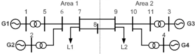
The first adopted test system corresponds to a simple multi-machine power system which was chosen with the purpose of clarifying the application of the proposed tool. Its single line diagram is shown in Fig. 6 and its complete data can be obtained in Kundur (1994).
Figure 6: Single line diagram of the test system 1.
PSSs were placed only in the generators G1 and G3, which, according to a residue analysis (Pagola et al., 1989; Martins and Lima, 1990), is enough to properly damp the power sys-tem electromechanical modes. Table 1 shows the eigenvalues related to the electromechanical modes of the test system 1, in the base case condition, with the two PSSs. The PSSs placed in the test system 1 were taken from the literature and therefore details regarding the design of these controllers may be obtained in Kundur (1994). The eigenvalues of test system 1 in open-loop (without the PSSs) and the transfer functions of the system PSSs can be found in the appendix. It is important to emphasize that the design of PSS is not the aim of this work, since the proposed approach was formu-lated to generate robust parameter ranges for the field tuning of PSS previously designed by some design methodology.
Table 1: Eigenvalues corresponding to the electromechanical modes of test system before the PSS retuning.
Oscillations Modes
Eigenvalues (1/s)
Damping Ratio (%) Inter-area −0.27±j3.77 7.22
Local −1.23±j7.09 17.12
Local −1.26±j7.35 16.86
power variation was distributed among all system generators, weighted by their corresponding inertia constants.
A damping ratio of 5% was initially sought as desired small-signal stability margin for the power system with the retuned controller. The algorithm took 9 iterations and the resulting range of parameter value is depicted in Fig. 7. Each iteration, corresponding to the solution of LMIs (22)-(24), was carried out using the solver ‘mincx’, available in the LMI Toolbox of MATLAB (Gahinet et al., 1995), and the whole iterative process took about 18 minutes in a computer equipped with an i7 3.0 GHz processor and 8GB of RAM memory. This same computer is also employed in all the subsequent tests.
In the sequence, the parameter range was recalculated con-sidering a damping ratio of 10% for the response modes of the power system with the retuned controller. The algorithm took about 10 minutes (corresponding to 5 iterations) to pro-vide a solution. The resulting parameter range is also de-picted in Fig. 7, considering also the algorithm evolution. Since the nominal value of the parameter (ρ1{o}= 20) is not
enough to provide a damping ratio higher than 10% for the system response modes, the algorithm was initialized with the maximum allowable value of gain (ρ1{o}= 50).
Accord-ing to the parameter ranges presented in Fig. 7, it is possi-ble to see that the engineer responsipossi-ble for the PSS tuning may employ static gain values from 16 to 50 p.u. (30 to 50 p.u.) with the assurance that the system will present response modes with damping ratio higher than 5% (10%) for the re-sponse modes of the power system.
0 5 10 16 20 24 28 30 32 34 36 38 40 42 44 46 48 50
4 5 6 7 8 9 10 11
Static Gain Kpss1 (p.u.)
Damping Ratio (%)
Parameter Range A Parameter Range B
ρ1{Final_min}
ρ1{Final_min} ρ1{0}
ρ
ρ
1{0}
1{Final_max}
Figure 7: Ranges of values for the retuning of the PSS at generator G3.
Fig. 8 shows the eigenvalues related to the closed-loop model of test system 1 with the retuned PSS, in the base case operat-ing condition, consideroperat-ing five different values of static gain belonging to the parameter range that ensures damping ratio higher than 5% (gains belonging to parameter range A pre-sented in Fig. 7). In Fig. 8, it is possible to verify that the five different values of static gain belonging to the generated
parameter ranges have assured a damping ratio higher than 5% for the response modes of the power system.
These five gain values, together with other ten gain values, were also evaluated considering the other employed operat-ing conditions. As expected, all the considered gain values provided the small-signal stability margin specified in the control problem formulation, in all operating conditions con-sidered.
It is worth mentioning that depending on the amount of PSSs placed in the system and which PSSs will be tuned, a given small-signal stability margin may not be achieved by a re-tuning procedure. In such case, new PSSs or simultaneous retuning of various system PSSs may be required to accom-plish the desired small-signal stability margin.
−3 −2.5 −2 −1.5 −1 −0.5 0
0 1 2 3 4 5 6 7 8 9
Real (1/s)
Imaginary (rad/s)
Kpss1=16 Kpss1=25 Kpss1=35 Kpss1=45 Kpss1=50
Inter−area Mode
5% Local Modes
Figure 8: Eigenvalues of the test system 1 after the applica-tion of the proposed tool, considering 5 different gain values for the retuning of the PSS at generator G3.
The approach was also employed to simultaneously gener-ate the parameter ranges for the two PSSs of test system 1. This evaluation took into account the same operating condi-tions and minimum damping ratios (5% and 10%) employed in the previous test. The parameter ranges were determined by the algorithm in 9 iterations for damping ratio of 5% (for which the overall process took about 2 hours and 12 min-utes) and 5 iterations for damping ratio of 10% (for which the overall process took about 1 hours and 6 minutes). The resulting parameter boxes are presented in Fig. 9. Analyzing the resulting parameter box A (box B) in Fig. 9, it is possible to see that the gains of the PSSs placed in generators G1 and G3 may be simultaneously set between 16 and 50 p.u. (30 and 50 p.u.) with the assurance of damping ratio higher than 5% (10%) for response modes of the power system with the retuned PSSs.
0 16 30 50 0
16 30 50
Static Gain Kpss2 (p.u.)
Static Gain Kpss1 (p.u.)
0
0
Parameter Box B
Parameter Box A
ζ =5% ζ =10%
Figure 9: Ranges of values for the retuning of the PSSs at generators G1 and G3.
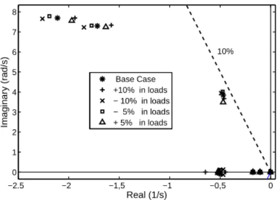
specified in the control problem formulation, in all consid-ered operating conditions. Fig. 10 presents the poles related to the electromechanical modes of the system in five different operating conditions, considering only one point belonging to parameter box B (Kpss1=37 and Kpss2=32). The anal-ysis presented in Fig. 10 shows that, after the retuning of the PSSs placed in generators G1 and G3, the test system 1 kept the small-signal stability margin specified in the control problem formulation for the five different operating condi-tions.
−2.5 −2 −1,5 −1 −0,5 0
0 1 2 3 4 5 6 7 8
Real (1/s)
Imaginary (rad/s)
Base Case +10% in loads − 10% in loads − 5% in loads + 5% in loads
10%
Figure 10: Eigenvalues of the test system 1 after the appli-cation of the proposed tool, considering 5 different operating conditions for the retuning of the PSSs at generators G1 and G3.
Nonlinear analyses, considering the power system before and after the PSS tuning, were also performed in order to validate the linear ones. Fig. 11 presents nonlinear response corre-sponding to the speed of generator G4, in a case where the loads were increased by 7.5% with respect to their base case levels. The retuning of the PSSs at generators G1 and G3 has improved the damping of the response modes observed in rotor speed of generator G4.
2 3 4 5 6 7 8 9 10
376.8 376.9 377 377.1 377.2 377.3 377.4 377.5 377.6
Time (s)
Rotor Speed (rad/s)
Kpss1=Kpss2=20 (Before tuning) Kpss1=40 − Kpss2=20 Kpss1=40 − Kpss2=40
Figure 11: Speed response of generator G4 considering the system operating with the PSSs before and after the retuning.
Different from the studies carried out in de Oliveira et al. (2010b), in this work the methodology is also applied to tune AVRs. After generating parameter ranges just for PSSs, the approach was employed to generate parameter ranges just for AVRs (with nominal PSSs in operation, but with their param-eters unchanged) and also for AVRs and PSSs, simultane-ously. This evaluation took into account a minimum damp-ing ratio of 5% and the same operatdamp-ing conditions employed in the previous test. Since the AVR gains are usually higher than the PSS gains, the calculation of the parameter ranges for the AVR consider gain deviations of 20 p.u. for the al-gorithm iterations (i.e.,∆ρ=20 p.u.). The nominal parame-ters of the AVRs employed in the model of test system 1 are Ke=200 p.u. and Te=0.01 s. Fig. 12 presents the parame-ter box deparame-termined for the simultaneous tuning of the AVRs placed in generators G1 and G3. The parameter box gener-ated for the simultaneous tuning of the AVR and PSS placed in generator G3 is presented in Fig. 13. Fig. 14 shows the eigenvalues related to the closed-loop model of test system 1, in the base case operating condition, after the retuning of the AVR and PSS (different values of static gains belonging to the parameter box presented in Fig. 13 were considered).
0 136 200 320 350
0 136 200 320 350
Static Gain Ke2 (p.u.)
Static Gain Ke1 (p.u.)
0 ζ =5%
Parameter Box
0 12 20 50 60 0
160 200 220 250
Static Gain Kpss1 (p.u.)
Static Gain Ke1 (p.u.)
0 ζ =5%
Parameter Box (PSS + AVR)
Figure 13: Ranges of values for the retuning of the PSS and AVR at generator G3.
Analyzing Fig. 12, it is possible to see that any values of
Ke_1andKe_2between 136 and 320 p.u. (i.e., any values
be-longing to resulting parameter box) assure the desired small signal stability margin for the power system (damping ratio higher than 5%) in all the considered operating conditions. It must be highlighted at this point that the lower limits in Fig. 12 were defined by nonlinear simulations that ensured a minimum steady-state error of 1% for the terminal voltages of both generators (otherwise, smaller gains could ensure the desired damping but not be practical, in the sense that they do not provide a satisfactory voltage regulation). The param-eter box presented in Fig. 13 shows that the static gain of the PSS and AVR placed in generator G3 may be simultaneously set from 12 to 50 p.u. and from 160 to 220 p.u., respectively (i.e.,12 ≤Kpss ≤50and160 ≤ Ke ≤ 220), with assur-ance of damping ratio higher than 5% for response modes of the power system with the retuned controllers. In Fig. 14, it is possible to notice that the different values of static gains belonging to the parameter box presented in Fig. 13 (PSS and AVR gains) assured the small-signal stability margin speci-fied in the control problem formulation.
−3 −2.5 −2 −1.5 −1 −0.5 0
0 2 4 6 8 10
Real (1/s)
Imaginary (rad/s) Kpss1=12 and Ke1=160
Kpss1=50 and Ke1=160
Kpss1=50 and Ke1=220
Local Modes 5%
Inter−area Mode
Figure 14: Eigenvalues of the test system 1 after the retuning of the PSS and AVR at generator G3, considering different gain values.
It is important to observe that the algorithm usually finds a conservative range due to the control formulation conser-vatism and numerical characteristics in the solver employed to resolve the LMIs. However, the parameter range found by the proposed tool always ensures the robustness and the specified small-signal stability margin for the power system with the retuned controllers.
In a second sequence of tests, the effectiveness of the pro-posed tool is evaluated in a larger power system correspond-ing to the reduced-order model of the New England system (Rogers, 2000). This system is constituted by 39 buses and 10 generators. The single line diagram of this system is shown in Fig. 15. Generator G10, shown in Fig. 15, is an equivalent of the New York system. The eigenvalues cor-responding to the 9 electromechanical modes of test system 2 in open- loop (without the PSSs) are presented in the ap-pendix.
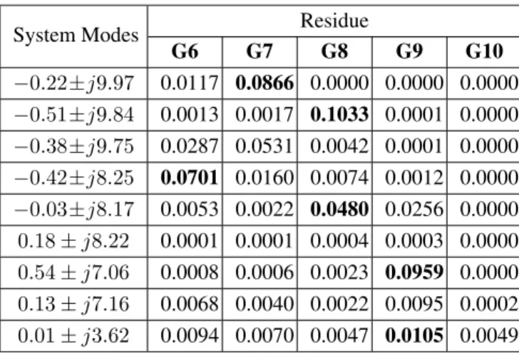
Again, a base case and two other operating points, related to variations of±10%in the values of the base case loads, were employed in these tests. A residue analysis has shown that 8 PSSs are enough to properly damp the electromechanical oscillations and provide a good small signal stability margin for the system. The absolute values of the residues related to the open-loop transfer function of test system 2, for each electromechanical mode, are presented in the appendix. The residues were calculated considering the transfer function be-tweenui (i-th stabilizing signal) andyi (speed deviation of the i-th generator). As result of this residue analysis, con-trollers were placed in generators G1, G2, G3, G4, G6, G7, G8 and G9 of test system 2.
The PSSs for test system 2 were designed taking into account the operating point regarding the base case. The design was based on the residue technique (Sadikovic et al., 2005; Fu-rini et al., 2011), which takes into account the coordination between the designed controllers. The PSSs were sequen-tially designed, which means that each of the controllers is designed one at a time. It is worth mentioning again that the design and placement of PSSs are not the focus of this work. The parameters of the PSSs placed in this test system are also presented in the appendix.
Figure 15: Single line diagram of test system 2.
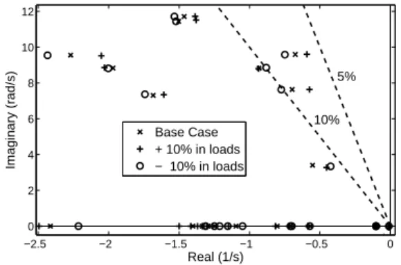
damped modes, considering the three operating conditions, are located between the two dashed lines of Fig. 16.
−2.5 −2 −1.5 −1 −0.5 0
0 2 4 6 8 10 12
Real (1/s)
Imaginary (rad/s)
Base Case + 10% in loads − 10% in loads
10% 5%
Figure 16: Eigenvalues of the test system 2 before the appli-cation of the proposed tool.
A modal analysis of the test system 2 has showed that con-troller placed in generator G4 presents the best controllabil-ity index to improve the damping of the two least damped modes. Based on this analysis, it was found that the state variables of the PSS at generator G4 had the highest partic-ipation factors with respect to the least damped modes and, therefore, the PSS of G4 was chosen as the one for retun-ing in this application of the proposed tool. The participation factors of the generator speed, in the least damped mode of the test system 2 (λ =-0,84+j10,93), are presented in the appendix. Damping ratios of 5% and 10% were sought as desired small-signal stability margins for the power system with the retuned PSS. The parameter ranges were determined by the algorithm in 12 iterations for a minimum damping ra-tio of 5% (for which overall iterative process took about 29
hours and 44 minutes) and 6 iterations for a minimum damp-ing ratio of 10% (for which the process took about 14 hours and 52 minutes). The resulting parameter ranges are pre-sented in Fig. 17. Analyzing Fig. 17, it is possible to see that the engineer in charge of the tuning of PSS placed in genera-tor G4 may set the controller gain between 4 and 50 p.u. (26 and 50 p.u.) with the assurance that the system will present response modes with damping ratio higher than 5% (10%).
0 4 8 26 50
4 5 6 7 8 9 10 11
Static Gain Kpss (p.u.)
Damping Ratio (%)
Parameter Range A Parameter Range B
Figure 17: Ranges of values for the retuning of the PSS placed in generator G4 of the test system 2.
The robustness of the resulting parameter ranges was vali-dated by means of linear and non-linear analyses. Fig. 18 shows the eigenvalues associated to the closed-loop models of the test system, for 4 different values of the PSS gain of generator G4 that are within the two ranges shown in Fig. 17. It can be seen that the desired small-signal stability margins of 5% and 10% are both satisfied when using these gains. Similar results were obtained for the system operating at low and high load levels, with respect to the base case.
Non-linear simulations before and after the retuning of the PSS of generator G4, were also carried out in order to val-idate the results observed in linear analysis. The speed re-sponse of generator G4 is presented in Fig. 19, in a case where the loads were increased by 7.5% with respect to their base case levels. The PSS retuning has significantly im-proved the damping of the modes of this speed response, which can be observed in Fig. 19.
stability, so he/she does not have to rely entirely on his/her judgment.
−2.5 −2 −1.5 −1 −0.5 0
0 2 4 6 8 10 12 14
Real (1/s)
Imaginary (rad/s)
Kpss1=26 Kpss1=30 Kpss1=40 Kpss1=50
10% 5%
Figure 18: Eigenvalues of the test system 2 after the appli-cation of the proposed tool, for 4 different gain values of the retuned PSS of generator G4.
2 3 4 5 6 7 8 9 10
376.6 376.8 377 377.2 377.4 377.6 377.8
Time (s)
Rotor Speed (rad/s)
G4 Speed − Kpss1=50 G4 Speed − Kpss1=26 G4 Speed − Kpss1=8
Figure 19: Speed response corresponding to generator G4 operating with the PSS before and after the retuning.
5
CONCLUSIONS
This paper presented a computational tool capable of gen-erating a range of parameter values to assist the engineers in charge of controller commissioning or retuning, in such a way that a guarantee of closed loop stability is provided for any gain adjustment made within this range. The main advantage of the application of this tool is the confidence it provides to the responsible engineer when approving a gain adjustment, during the commissioning stage, which is differ-ent from the one determined at the design stage based on the nominal model.
If the changes in the topology and/or operating conditions of the system (that can be extracted from the daily load curves and contingency lists for stability analysis, which are readily available at power system utilities) are adequately modeled in
the proposed tool, the engineer in charge of controller com-missioning does not have to rely entirely on his/her empirical knowledge about the system to perform the gain retuning in the field. It is also important to remark that, due to the possi-bility of application of the same technique to any parameter variation in the model, the same tool can be used to retune the phase compensation parameters of a PSS in order to provide a range of guaranteed small signal stability margin.
The results obtained with the tests have showed that the pro-posed tool successfully generated ranges of static gain val-ues for PSSs and AVRs that ensure stability robustness and the fulfillment of a minimum damping ratio criterion for the closed loop power system.
Future directions of this work include the application of this methodology to the tuning of other kinds of power system controllers. Different LMI formulations will also be inves-tigated in order to reduce the computational effort required to solve the control problem. Furthermore, the investigation of some model order reduction techniques, in order to find out the most suitable ones to be used in conjunction with this algorithm, is also a future direction of this research.
A
APPENDIX
The model of thei-th synchronous generator with its AVR is given by:
˙
δi=ωsωi−ωs, (A.1)
˙
ωi=
1 2H
[
Pmi−Eqi′ Iqi−E′diIdi−(x′di−x′qi)IdiIqi ]
,
(A.2)
˙
E′
qi=
1
τ′
doi [
(xdi−x′di)Idi+EF Di−Eqi′ ]
, (A.3)
˙
Edi′ =
1
τ′
doi [
(x′qi−xqi)Iqi−Edi′ ]
, (A.4)
˙
EF Di=
1
Tei
[Kei(Vref i− |Vti|+Vpssi)−EF Di], (A.5)
whereδis the generator power angle,ωis the rotor angular speed, ω0 is the synchronous machine speed,E′d is the
di-rect axis transient voltage,E′qis the quadrature axis transient voltage,Iqis the quadrature axis current,Idis the direct axis current,EF Dis the voltage applied to the field circuit by the AVR,Vtis terminal voltage,Vrefis the reference voltage for the AVR, andVpssis the stabilizing signal from the PSS.
˙
x1=Kpssω˙ −
1
Tw
x1, (A.6)
˙
x2= 1
T2
[x1+T1x˙1−x2], (A.7)
˙
Vpss=
1
T2
[x2+T1x˙2−Vpss]. (A.8)
In (A.6)-(A.8),x1,x2, andVpss are the state variables re-lated to the PSS model. Additional details regarding the sys-tem model and its respective parameters can be obtained in Kundur (1994), Anderson and Fouad (2003), and Machowski et al. (2008).
The eigenvalues related to the electromechanical modes of the test system 1 without PSSs are presented in Table A.1 and the transfer function corresponding to the PSSs placed in test system 1 is given by
Fpss1(s) =Fpss2(s) =
= 20 (10s)(0.05s+ 1)(3.00s+ 1)
(10s+ 1)(0.02s+ 1)(5.40s+ 1). (A.9)
Table A.1: Eigenvalues corresponding to the electromechan-ical modes of test system before the PSS retuning.
Oscillations Modes
Eigenvalues (1/s)
Damping Ratio (%)
Inter-area 0.06±j3.55 -1.80
Local −0.42±j6.82 6.14
Local −0.40±j7.05 5.64
The absolute values of the residues related to the open-loop transfer function of test system 2, for each electromechanical mode, are presented in Tables A.2 and A.3.
The absolute values of the participation factors of the gen-erator speed in the least damped mode of the test system 2 are presented in Table A.4. The speed of the generator was chosen due to the fact that the electromechanical oscillations usually have a strong participation on this variable.
The parameters of the existing PSSs in the test system 2 be-fore retuning are presented in Table A.5. Note that, after the retuning suggested by the proposed tool, any Kpss in the range between 4 p.u. and 50 p.u. can be used, and the system will still present a 5% minimum damping as a small-signal stability margin. The engineer in charge of the PSS retuning can then confidently choose, using his/her own judgment, the
Table A.2: Eigenvalues corresponding to the electromechani-cal modes of test system 2 in open-loop and absolute values of the residues regarding the generators G1 to G5.
System Modes Residue
G1 G2 G3 G4 G5
−0.22±j9.97 0.0001 0.0000 0.0001 0.0862 0.0141 −0.51±j9.84 0.0161 0.0001 0.0001 0.0016 0.0009 −0.38±j9.75 0.0007 0.0001 0.0003 0.0813 0.0346 −0.42±j8.25 0.0018 0.0005 0.0004 0.0043 0.0431 −0.03±j8.17 0.0140 0.0080 0.0043 0.0032 0.0113
0.18±j8.22 0.0001 0.0542 0.0689 0.0001 0.0002
0.54±j7.06 0.0003 0.0122 0.0137 0.0017 0.0023
0.13±j7.16 0.0010 0.0258 0.0228 0.0194 0.0347
0.01±j3.62 0.0040 0.0051 0.0066 0.0089 0.0094
Table A.3: Eigenvalues corresponding to the electromechani-cal modes of test system 2 in open-loop and absolute values of the residues regarding the generators G6 to G10.
System Modes Residue
G6 G7 G8 G9 G10
−0.22±j9.97 0.0117 0.0866 0.0000 0.0000 0.0000 −0.51±j9.84 0.0013 0.0017 0.1033 0.0001 0.0000 −0.38±j9.75 0.0287 0.0531 0.0042 0.0001 0.0000 −0.42±j8.25 0.0701 0.0160 0.0074 0.0012 0.0000 −0.03±j8.17 0.0053 0.0022 0.0480 0.0256 0.0000
0.18±j8.22 0.0001 0.0001 0.0004 0.0003 0.0000
0.54±j7.06 0.0008 0.0006 0.0023 0.0959 0.0000
0.13±j7.16 0.0068 0.0040 0.0022 0.0095 0.0002
0.01±j3.62 0.0094 0.0070 0.0047 0.0105 0.0049
best value of gain within this range that suits other practical requirements as well, such as the avoidance of saturation of PSS outputs when responding to typical perturbations, for example.
ACKNOWLEDGEMENTS
Table A.4: Absolute values of the participation factors of the generator speed in the least damped mode of the test system 2 with the 8 PSSs.
Generator Variable Participation Factors
(λ=−0.84 +j10.93)
G1 ωG1 0.0022
G2 ωG2 0.0002
G3 ωG3 0.0009
G4 ωG4 0.3229
G5 ωG5 0.0727
G6 ωG6 0.0176
G7 ωG7 0.0037
G8 ωG8 0.0001
G9 ωG9 0.0003
G10 ωG10 0.0000
Table A.5: Parameters of the Existing PSSs in the Test Sys-tem 2 before Retuning of the PSS in G4.
Generator Tw (s) Kpss
(p.u.)
T11(s) (nc= 2)
T21(s) (nc= 2)
G1 10 8.00 0.2111 0.1044
G2 10 9.00 0.2200 0.1505
G3 10 9.00 0.2004 0.1773
G4 10 8.00 0.1973 0.1329
G6 10 10.00 0.2075 0.1656
G7 10 9.00 0.2096 0.1537
G8 10 8.00 0.1709 0.1127
G9 10 9.00 0.2051 0.1005
REFERENCES
Abdel-Magid, Y. and Abido, M. (2003). Optimal multiob-jective design of robust power system stabilizers using genetic algorithms, IEEE Transactions on Power Sys-tems18(3): 1125–1132.
Anderson, P. and Fouad, A. (2003). Power System Control and Stability, IEEE Press, New York - NY.
Bomfim, A., Taranto, G. and Falcao, D. (2000). Simultane-ous tuning of power system damping controllers using genetic algorithms, IEEE Transactions on Power Sys-tems15(1): 163–169.
Cai, L.-J. and Erlich, I. (2005). Simultaneous coordinated tuning of pss and facts damping controllers in large
power systems, IEEE Transactions on Power Systems
20(1): 294–300.
Chilali, M., Gahinet, P. and Apkarian, P. (1999). Robust pole placement in lmi regions,IEEE Transactions on Auto-matic Control44(12): 2257–2270.
de Oliveira, R. V., Ramos, R. A. and Bretas, N. G. (2010a). An algorithm for computerized automatic tuning of power system stabilizers,Control Engineering Practice
18(1): 45–54.
de Oliveira, R. V., Ramos, R. A. and Bretas, N. G. (2010b). Ferramenta para ajuste robusto de controladores de amortecimento para sistemas eltricos de potncia,Anais do XVIII Congresso Brasileiro de Automtica, Bonito, MS, Brasil, pp. 1894–1900.
Furini, M., Pereira, A. and Araujo, P. (2011). Pole placement by coordinated tuning of power system stabilizers and facts-pod stabilizers, International Journal of Electri-cal Power & Energy Systems33(3): 615–622.
Gahinet, P., Apkarian, P. and Chilali, M. (1996). Affine parameter-dependent lyapunov functions and real para-metric uncertainty, IEEE Transactions on Automatic Control41(3): 436–442.
Gahinet, P., Nemirovski, A., Laub, A. J. and Chilali, M. (1995). LMI control toolbox user’s guide, The Math-works Inc.
Gomes, S., J., Martins, N. and Portela, C. (2003). Com-puting small-signal stability boundaries for large-scale power systems, IEEE Transactions on Power Systems
18(2): 747–752.
Gurrala, G. and Sen, I. (2010). Power system stabilizers de-sign for interconnected power systems,IEEE Transac-tions on Power Systems25(2): 1042–1051.
Jabr, R., Pal, B., Martins, N. and Ferraz, J. (2010). Robust and coordinated tuning of power system stabiliser gains using sequential linear programming,IET Generation, Transmission Distribution4(8): 893–904.
Kundur, P. (1994). Power system stability and control, EPRI Editors, McGraw-Hill, New York, NY.
Machowski, J., Bialek, J. W. and Bumby, J. R. (2008).Power System Dynamics - Stability and Control, John Wiley & Sons, Chichester, UK.
Oliveira, R. C. and Peres, P. L. (2005). Stability of poly-topes of matrices via affine parameter-dependent lya-punov functions: Asymptotically exact lmi conditions,
Linear Algebra and its Applications405(1): 209–228.
Pagola, F., Perez-Arriaga, I. and Verghese, G. (1989). On sensitivities, residues and participations: applica-tions to oscillatory stability analysis and control,IEEE Transactions on Power Systems4(1): 278–285.
Perez-Arriaga, I., Verghese, G. and Schweppe, F. (1982). Selective modal analysis with applications to electric power systems, part i: Heuristic introduction, IEEE Transactions on Power Apparatus and Systems PAS– 101(9): 3117–3125.
Ramos, R. A. (2009). Stability analysis of power sys-tems considering avr and pss output limiters, Interna-tional Journal of Electrical Power & Energy Systems
31(4): 153–159.
Rogers, G. (2000). Power system oscillations, Kluwer, Norwell-MA.
Sadikovic, R., Korba, P. and Andersson, G. (2005). Appli-cation of facts devices for damping of power system oscillations,IEEE Russia Power Tech, 2005, pp. 1 –6.
Verghese, G., Perez-Arriaga, I. and Schweppe, F. (1982). Selective modal analysis with applications to electric power systems, part ii: The dynamic stability problem,
IEEE Transactions on Power Apparatus and Systems
PAS-101(9): 3126–3134.
Zanchin, V. and Bazanella, A. (2003). Robust output feed-back design with application to power systems, 42nd IEEE Conference on Decision and Control, 2003. Pro-ceedings., Vol. 4, pp. 3870–3875.