Vol. 33, No. 01, pp. 145 - 153, January - March, 2016 dx.doi.org/10.1590/0104-6632.20160331s00002846
ROBUST CONTROL OF WIENER SYSTEMS:
APPLICATION TO A pH NEUTRALIZATION
PROCESS
S. I. Biagiola, O. E. Agamennoni
1and J. L. Figueroa
* Instituto de Investigaciones en Ingeniería Eléctrica –IIIE (UNS-CONICET),Departamento de Ingeniería Eléctrica y de Computadoras, Universidad Nacional del Sur,
Avda. Alem 1253, (8000) Bahía Blanca, Argentina. Phone: + 54 291 4595101 ext. 3325, Fax: + 54 291 4595154
E-mail: [email protected]
(Submitted: July 18, 2013 ; Revised: February 6, 2015 ; Accepted: February 21, 2015)
Abstract - In this paper, the robustness of a typical control scheme for Wiener systems is studied. These systems consist of the cascade connection of a linear time invariant system and a static nonlinearity. To control this kind of systems, several approaches were discussed in the literature. Most of these control schemes involve transformation of the measured variable as well as the setpoint, by the inverse of the nonlinear gain. The approach followed in this work uses the inverse model of the static nonlinear gain, while the uncertainty in the Wiener model is treated as a partitioned problem. The linear block is considered as a parameter-affine-dependent model and, on the other hand, the nonlinear block uncertainty is analyzed as a conic-sector. The robustness analysis is performed using -theory. The results are evaluated on the basis of a simulation of a pH neutralization process.
Keywords: Wiener Models; Process Control; Uncertainty; Robustness.
INTRODUCTION
Many contributions for controller design are based on the assumption of a linear model of the system. However, in some cases it is difficult to represent a given process using a linear model. This situation takes place, for example, when a highly nonlinear system undergoes operating point changes along a wide region. For this reason, in the last decades, there has been much interest in nonlinear model-based control within the chemical engineering com-munity. A critical step in the application of these methods is the development of a suitable model of the process dynamics. In this sense, Sjöberg et al.
(1995) describe several approaches for model devel-opment and this approach can be specially appealing
as regards control process applications. In particular, the Wiener model (WM) can be mentioned (Pearson and Pottmann, 2000) due to its wide diffusion and applicability in control. The WM consists of a cas-cade connection of a linear time invariant (LTI) sys-tem followed by a static nonlinearity.
A highly cited paper regarding Wiener model iden-tification is the contribution by Gómez and Baeyens (2004), in which noniterative algorithms for the iden-tification of both multivariable Hammerstein and Wiener systems were developed. Rational orthonor-mal bases were considered for the representation of the linear subsystem in the case of the Wiener model.
In most of the control applications of Wiener Models, the underlying strategy involves the inverse of the nonlinearity, such as in the works by Gerkšič
et al. (2000), Bloemen et al. (2001a) and Gómez and Baeyens (2000, 2004).
Although much research effort has been dedicated to Wiener models, to the best of our knowledge, a systematic robustness analysis for this scheme under uncertainty has not been developed in the literature.
Since Wiener models could be approximations of the real process, the robustness of the designed con-trol structure may deserve analysis. In order to apply robust control theory, one needs not only a nominal process model, but also a suitable description of the modeling errors, which are typically in the form of some bounds of parameter variations (Wang and Ro-magnoli, 2003). The classical robust control analysis and design methodologies are based on linear models (Doyle, 1982). As regards techniques for robust non-linear control, they usually consist of covering the nonlinearity by an affine convex hull and, then, to perform the analysis on it (Popov, 1962; Bloemen et al., 2001b). However, a dedicated controller design and robustness analysis should be developed for pro-cesses approximated by Wiener models.
In this article, an analysis of the robustness of closed loop Wiener Systems is performed. The un-certainty in the Wiener model is treated as a parti-tioned problem. The linear block is considered as a parameter-affine-dependent model, which is suitable for Lyapunov-based analysis. Therefore, the stated stability problem can be dealt with as a sector bounded uncertainty problem and easily converted to a linear fractional uncertainty model. On the other hand, the nonlinear block uncertainty is analyzed as a conic-sector. The robustness analysis is performed using -theory.
To illustrate the proposed control strategy, a pH neutralization process is selected herein. This pro-cess has been widely recognized in the literature as a challenging problem due to the highly nonlinear and time-varying dynamic nature. From the perspective of system identification, pH processes have often been considered in the literature as having a Wiener structure (Kalafatis et al., 1995). Different Wiener representations have been favorably used for the
pur-these works, we mention the paper by Kalafatis et al. (2005a), in which they evaluated the control of pH processes based on the Wiener model structure, where the static nonlinearity was assumed to represent the titration curve. Moreover, assessment of the condi-tions under which the pH process behaves like an exact Wiener system was accomplished. A simple linearizing feedforward controller was proposed based on an estimation of the inverse titration curve.
Along the same line, Gómez and Baeyens (2004) illustrated the suitability of the proposed methods in the identification of the pH neutralization process. They recognized this dynamic system as a bench-mark drawn from the process control literature.
More research work on this subject is due to Mahmoodi et al. (2009). They employed Laguerre filters and polynomial functions as the linear and nonlinear blocks of the Wiener model, respectively. The so-called Wiener-Laguerre model was used to evaluate identification and nonlinear model predic-tive control of a pH neutralization process.
It must be remarked that, although the study herein developed is in the context of a pH neutraliza-tion reactor control, the conclusions can be directly extended to any other application.
The paper is organized in the following way. In the next section the process description is given. A Wiener model (and the related uncertainty) is then developed. The controller is designed and the simu-lation results are presented. The paper concludes with some final remarks.
PROCESS DESCRIPTION
The control of a pH neutralization processes is a relevant topic in several industries, such as wastewater treatment, pharmaceuticals production, bioprocesses plants, and chemical processing. It is often difficult to achieve a high performance and robust pH control due to their time-varying and severe nonlinear char-acteristics (Henson and Seborg, 1994). Therefore, pH control is frequently conceived as the unavoidable case study for the assessment of novel modeling and control strategies. Actual research work confirms that this process is still interpreted as a control bench-mark (Mahmoodi et al., 2009; Wang and Zhang, 2011; Kim et al., 2012).
solution of composition x1i(t) and a time-varying
volu-metric flow qA(t) is neutralized using an alkaline
so-lution of volumetric flow qB(t) and known
composi-tion made up of base x2i and buffer agent x3i. The
nominal values for qA and qB are 1 and 0.5 L/min,
respectively. Due to the high reaction rates of the acid-base neutralization, chemical equilibrium condi-tions are instantaneously achieved. Moreover, under the assumptions that the acid, the base and the buffer are strong enough, then the total dissociation of the three compounds takes place.
The process dynamic model can be obtained by considering the electroneutrality condition (which is always preserved) and through mass balances of equivalent chemical species (known as chemical in-variants) that were introduced in Gustafsson and Waller (1983). For this specific case, under the previ-ous assumptions, the dynamic behavior of the pro-cess can be described considering the state variables:
x1=[A-], x2=[B+] and x3=[X-]. Therefore, the mathe-matical model of the process can be written in the following way (Galán, 2000):
1 1 1
( )
A A B
i
q q q
x x x
V V
(1)
2 2 2
( )
B A B
i
q q q
x x x
V V
(2)
3 3 3
( )
B A B
i
q q q
x x x
V V
(3)
2 3 1
3 ( , )
0
1 /
w
x w
K
F x x x x
x
K K
(4)
where =10-pH. Kw and Kx are the dissociation
con-stants of the buffer and the water, respectively. The parameters of the system represented by Equations (1)-(4) are addressed in Table 1. Equation (4) was
deduced by McAvoy et al. (1972), and it takes the standard form of the widely used implicit expression that connects pH with the states of the process.
Now, making xx2x1, it is possible to reduce the process model to:
2 1
( )
B A A B
i i
q q q q
x x x x
V V V
(5)
3 3 3
( )
B A B
i
q q q
x x x
V V
(6)
3 3
3 ( , , )
0
1 /
w
x w
K
F x x x x
x
K K
(7)
Table 1: Neutralization Parameters.
Parameter Value
x1i 0.0012 mol HCl/l
x2i 0.0020 mol NaOH/l
x3i 0.0025 mol NaHCO3/l
Kx 10-7 mol/l
Kw 10-14 mol2/l2
qA 1 l/m
V 2.5 l
WIENER MODEL
Figure 1 depicts a Wiener model. It consists of a LTI system described in a state space form (this de-scription for the linear block was used by, for exam-ple, Bruls et al. (1999), Westwick and Verhaegen (1996) and Lussón Cervantes et al. (2003)) (A,B,C) followed by a static nonlinearity N(.). That is, the linear model maps the input signal qB( )t into the intermediate variable v(t), and the overall model out-put is y(t)=N(v(t)). In this scheme, the bar over qB
means deviation: i.e., qB qBqB s, , where qB,s stands
for the steady-state value of this physical variable.
) (t
qB v(t)
y
(
t
)
( ) ( ) ( ) ( ) ( )
B
t A t Bq t
v t C t
(.)
N
In this case, the relation between the input and the output is represented by the following model:
( ) ( ) ( )
( ) ( ) B
t A t Bq t
v t C t
(8)
where the linear description of the process results from a linearization around the steady state
Ts A B B i A B A i B i
s x q x q q q x q q q
x 2 1 3 . The
output variable y(t) is the deviation variable for the measured pH. Note that Equation (7) can be rewrit-ten as the following third-order polynomial:
3 2 3 3 2 ( , , ) 0 w x w w x x x Kh x x x x
K K K x K K K (9)
Then, the resulting linear model is:
2 1 3 2 2 0 0 0 ln(10) ln(10)i i A
B A
B A
B A i A
B A
x w x
x x q
q q
V V q q
A B q q x q
C D V V q q
K K K
dh dh d d where
3 33 2 w x w
x x
K K
h
x x x K
K K
Note that computation of the following linear model matrix in the steady-state
s C B A 0
involves the entries of the matrices (A,B,C) that must be evaluated for qB=qB,s, qA=qA,s, x1i= x1i,s, x2i= x2i,s,
x3i= x3i,s, pH=pHs.
The nominal linear model is computed at qB,s=0.5.
Then, to determine the values for the static nonlinear gain, the values of q are varied in the range [0,1].
This also implies that the linear model will differ from the nominal one. To cope with these changes, the following proposals are considered: a) the linear model includes uncertainties in the entries of the ma-trices (A,B,C) and b) the nonlinear gain is charac-terized (i.e., no uncertainty is present in it).
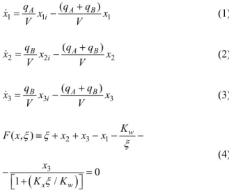
The influence of qB values on the LTI model
pa-rameters was determined and the results are shown in Figure 2.
Figure 2: Parameters of the linear model as a func-tion of qB.
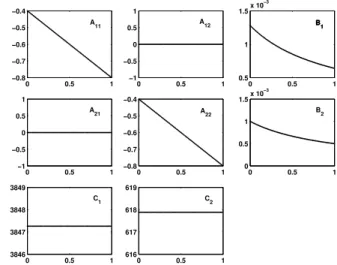
As regards the characterization of the static non-linear gain, the titration curve is approximated by means of a Piecewise Linear (PWL) function. PWL functions have proved to be a very powerful tool in the modeling and analysis of nonlinear systems (Chua and Ying, 1983). The general formulation of PWL functions allows us to represent a continuous nonlinear function through a set of linear expres-sions, each of them valid in a certain operation re-gion. To make this approximation, the range of input variables v (i.e., ) is partitioned into a set of non-empty regions i, such that
1 i i
. In each of these regions, the non-linear function is approxi-mated using a linear (affine) representation. These functions allow the development of a systematic and accurate treatment of the approximation.
It can be proved (Julián et al., 1999) that any con-tinuous nonlinear function N(v): m1 can be uniquely represented using the PWL functions as
1 0 , i i iy f v
(10)0 0.5 1
−0.8 −0.7 −0.6 −0.5 −0.4
0 0.5 1
−1 −0.5 0 0.5 1
0 0.5 1
0.5 1 1.5x 10
−3
0 0.5 1
−1 −0.5 0 0.5 1
0 0.5 1
−0.8 −0.7 −0.6 −0.5 −0.4
0 0.5 1
0 0.5 1 1.5x 10
−3
0 0.5 1
3846 3847 3848 3849
0 0.5 1
616 617 618 619
A11 A12 B1
A21 A22
B1
B2
where i are given parameters that define the
parti-tion of the domain of v, and are functions that in-volve nested absolute values (Julián et al., 1999).
Figure 3 depicts the real curve for the nonlinear gain, as well as the PWL approximation. The pa-rameters identification of the PWL model in Eq. (10) is accomplished using the pH data and the v(t) data obtained with Eq. (8). Therefore, for this pH neu-tralization model description the identified parame-ters are: N=[-3, -1.5, -1.2, 0.4, 1, 3]T, where the superscript N means that this partition is used to represent the gain N.
Figure 3: Nonlinear gain.
WIENER SYSTEM CONTROL
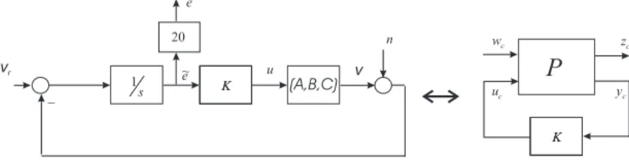
Wigren (1990) presented a structure for the control of Wiener systems. In this scheme (see Figure 4),
two static nonlinearities are included in the loop. Under the hypothesis that N(.) is invertible, the natural selection for the controller nonlinear func-tions is f(.)N-1(.). Note that this is the case of the pH neutralizer.
Figure 4: The closed loop scheme for Wiener Model.
Now, the controller design involves two steps: a) the inversion of the nonlinear gain and, b) the com-putation of a LTI controller in order to compensate for the linear block model of the process.
To compute f(.) we approximate it using a PWL function (Lussón Cervantes et al., 2003); Figure 5 shows this function. The partition of the f-domain is defined as f= [2.5, 3.8, 6.5, 8, 10]T, which corre-sponds to the partition of the pH range.
As mentioned above, the linear controller K
should be designed to compensate for the behavior of the linear dynamic block of the process model. This controller could be designed using any of the classi-cal techniques found in the literature. In our case, we use the H methodology (Gahinet et al., 1995). Let
us consider the reduced loop (i.e., the nonlinearity is excluded) of Figure 6. In this case, the design signals are uc=[u], yc=e~, wc=[vr n]T and zc=[e u] T. The
design transfer function is then
(A,B,C)
vr v
Figure 6: The closed loop scheme for the linear block.
1 2
1 11 12
2 21 22
0 0 0
0 1 1 0
0 20 0 0 0
0 0 0 0 1
0 1 0 0 0
p p
P
p p p
p p p
A B
A B B C
C D D
C D D
The controller (AK, BK, CK) is designed to reduce
the norm of the transfer function between wc and zc,
then the integral action (1/s) is included in the con-troller expression. Note that in this formulation we are minimizing the H norm between the set point
input (vr) and the measurement noise (n) to the
weighed integrated error (e) and the manipulated variable (u) signals. This minimization is performed using the function hinfsyn (Gahinet et al., 1995) that implements the algorithm defined by Doyle et al. (1989). It is important to note the significance of considering the measurement noise because its exist-ence in the complete scheme (which includes the static nonlinearity) could produce a mismatch be-tween the PWL sector of N and the PWL sector of f.
The robustness of this controller is tested against all the uncertainty sources: the linear model
parame-ters variation (Fig. 2), the conic sector of the nonlinear gain model (Fig. 3) and the conic sector related to the controller (Fig. 5). The system used for robustness analysis is described in Figure 7. This analysis is performed using -tools (Gahinet et al., 1995) with
=diag{A, B, N, f} (the uncertainty f in the
forward line does not affect the stability) and the following M- structure:
0 0
0 0
0 0 0 0 0
0 0 0 0 0
0 0 0 0 0
0 0 0 1 0
K
K K K K
M M
M M
K
A BC I I
B C f N A B f B
A B I
C
C D
C C N
In these expressions, the nominal values N (and
f) are computed as the average of the conic sector of Fig. 3 and Fig. 5, and the magnitude of the uncertain-ties depends on the variation of the entries of A, B and the respective conic sectors. Under these definitions, the closed loop becomes robustly stable (=0.74).
Figure 8 shows the simulation results for setpoint changes. Note that the system follows the setpoint with smooth changes in the manipulated variable, even under the wide excursion of the reference sig-nal. An interesting point is that, when we try to fol-low the same setpoint using only the linear controller (i.e., without considering the block f in the feedback loop), the system becomes unstable due to the sig-nificant nonlinearity of the process.
Two additional tests are performed; first we con-sider the effect of the measurement noise. A Gauss-ian noise of varGauss-iance 0.05 is added to the pH out-put. The simulation results are shown in Figure 9. It is important to mention that, when noise vari-ance increases, the performvari-ance of the controller deteriorates and the control system could become unstable.
Figure 8: Closed loop simulations.
Figure 9: Closed loop simulations for noisy meas-urement.
In what follows, the effect of perturbations is evaluated. When load changes are applied to the pro-cess, a fixed Wiener model no longer represents ade-quately the process. For example, the titration curve changes drastically (Kalafatis et al., 2005a; 2005b). To perform a robustness analysis in this case, we con-sider that qA varies between 0.8 and 1.2 and that x1i
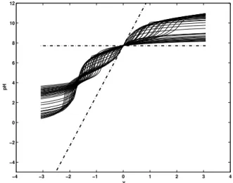
varies between 0.0008 and 0.0014. The effects of these changes on the LTI model parameters and the nonlinear gain are shown in Figure 10 and Figure 11, respectively. From these plots, it is clear that the model uncertainties increase. For this level of uncertainty the system is no longer robustly stable (=1.147).
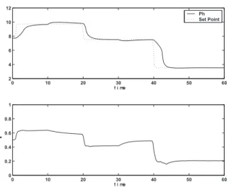
A simulation to evaluate the influence of lower perturbations is shown in Figure 12. In this case, qA
is reduced to 0.9 at t=10 min and x1i is increased to
0.0014 at t=30 min.
0 0.5 1
−1 −0.8 −0.6 −0.4 −0.2
0 0.5 1
−1 −0.5 0 0.5 1
0 0.5 1
0 0.5 1 1.5x 10
−3
0 0.5 1
−1 −0.5 0 0.5 1
0 0.5 1
−1 −0.8 −0.6 −0.4 −0.2
0 0.5 1
0 0.5 1 1.5x 10
−3
0 0.5 1
3846 3847 3848 3849
0 0.5 1
616 617 618 619
A11 A12
A21 A22
B1
B2
C1 C2
Figure 10: Parameters of the linear model as a func-tion of qB for different values of qA and x1i.
−4 −3 −2 −1 0 1 2 3 4
−4 −2 0 2 4 6 8 10 12
v
pH
Figure 11: Nonlinear gain for different values of qA
Figure 12: Closed loop simulations under perturbation.
CONCLUSIONS
In this article, controller design as well as robust-ness analysis of Wiener systems were considered. Wiener systems modeling and control were treated in the context of the more realistic case in which differ-ent sources of uncertainty are presdiffer-ent. For this pur-pose, PWL approximating functions were introduced. As regards the modeling and control approaches proposed in this work, PWL functions proved to be an appropriate and simple tool for uncertainty inclusion, nonlinearity modeling and nonlinearity inversion.
A design technique for the controller synthesis was also proposed. It makes use of well-known tools based on H theory, and it was shown to be a suitable
method for the uncertain feedback structure proposed herein. Stability aspects of the closed loop system under uncertainty were also dealt with using -theory. The different topics developed were tackled together in an application example of significant complexity.
ACKNOWLEDGMENTS
This work was financially supported by the Agen-cia Nacional de Promoción Científica y Tecnológica, CONICET, CIC and Universidad Nacional del Sur, Bahía Blanca, Argentina.
REFERENCES
Biagiola, S. I., Agamennoni, O. E. and Figueroa, J. L.,
H Control of a Wiener type system. International
Bloemen, H. H. J., Chou, C. T., van den Boom, T. J. J., Verdult, V., Verhaegen, M. and Backx, T. C., Wiener model identification and predictive con-trol for dual composition concon-trol of a distillation column. Journal of Process Control, 11(6), 601-620 (2001a).
Bloemen, H. H. J., van den Boom, T. J. J. and Ver-bruggen, H. B., Model-based predictive control for Hammerstein–Wiener systems. International Jour-nal of Control, 74, 482-495 (2001b).
Bruls, J., Chou, C. T., Haverkamp, B. R. J. and Ver-haegen, M., Linear and non-linear system iden-tification using separable least-squares. European Journal of Control, 5, 116-128 (1999).
Chua, L. O. and Ying, L. P., Canonical piecewise-linear analysis, IEEE transactions on circuits and systems. CAS-30, 125-140 (1983).
Cheong, M. Y., Werner, S., Cousseau, J. and Laakso, T., Predistorter identification using the simplicial canonical piecewise linear function. 12th Interna-tional Conference on Telecommunications, Cape Town, South Africa (2005).
Doyle, J. C., Analysis of feedback systems with struc-tured uncertainties. IEE Proceedings – Part D, 129(6), 242-250 (1982).
Doyle, J. C., Glover, K., Khargonekar, P. and Francis, B., State-space solutions to standard H2 and H
control problems. IEEE Transactions on Auto-matic Control, 34, 831-847 (1989).
Gahinet, P., Nemirovski, A., Laub, A. J. and Chilali, M., LMI Control Toolbox, The MathWorks. The MathWorks Inc., Natick, MA, USA (1995). Galán, O., Robust multi-linear model-based control
for nonlinear plants. PhD Thesis, University of Sydney, Australia (2000).
Galán, O., Romagnoli, J. A. and Palazoglu, A., Real-time implementation of multi-linear model-based control strategies: An application to a bench-scale pH neutralization reactor. Journal of Process Con-trol, 14, 571-579 (2004).
Gerkšič, S., Juričic, D., Strmčnic, S. and Matko, D., Wiener model based nonlinear predictive control. International Journal of Systems Science, 31, 189-202 (2000).
Gómez, J. C. and Baeyens, E., Identification of mul-tivariable Hammerstein systems using rational or-thonormal bases. Proceedings of the 39th IEEE Conference on Decision and Control, Sydney, Australia, 3, 2849-2854 (2000).
and reaction invariant control of pH. Chemical Engineering Science, 38, 389-398 (1983).
Henson, M. and Seborg, D., Adaptive nonlinear con-trol of a pH neutralization process. IEEE Trans. Control Syst. Technol., 2, 169-182 (1994). Hunter, I. W. and Korenberg, M. J., The
identifica-tion of nonlinear biological systems: Wiener and Hammerstein cascade models. Biological Cyber-netics, 55(2-3), 135-144 (1986).
Julián, P., Desages, A. C. and Agamennoni, O. E., High level canonical piecewise linear representa-tion using a simplicial partirepresenta-tion. IEEE Transac-tions on Circuits and Systems, CAS-46, 463-480 (1999).
Kalafatis, A., Arifin, N., Wang, L. and Cluett, W. R., A new approach to the identification of pH pro-cesses based on wiener model. Chemical Engi-neering Science, 50, 3693-3701 (1995).
Kalafatis, A. D., Wang, L. and Cluett, W. R., Linear-izing feedforward-feedback control of pH pro-cesses based on the Wiener Model. Journal of Process Control, 15, 103-112 (2005a).
Kalafatis, A. D., Wang, L. and Cluett, W. R., Identifi-cation of time-varing pH processes using sinusoi-dal signals. Automatica, 41, 385-691 (2005b). Kang, H. W., Cho, Y. S. and Youn, D. H., Adaptive
precompensation of Wiener systems. IEEE Trans-actions on Signal Processing, 40(10), 2825-2829 (1998).
Kang, H. W., Cho, Y. S. and Youn, D. H., On com-pensating nonlinear distortions of an OFDM sys-tem using an efficient adaptive predistorter. IEEE Transactions on Communications, 47(4), 522-526 (1999).
Kim, K. K., Ríos-Patrón, E. and Braatz, R. D., Robust nonlinear internal model control of stable Wiener systems. Journal of Process Control, 22, 1468-1477 (2012).
Korenberg, M. J., Identification of biological cas-cades of linear and static nonlinear systems. 16th. Proc. IEEE Midwest Symposium on Circuit The-ory, p. 1-9 (1973).
Lussón Cervantes, A., Agamennoni, O. E. and Figueroa, J. L., A nonlinear model predictive con-trol scheme based on Wiener piecewise linear models. Journal of Process Control, 13, 655-666 (2003).
Mahmoodi, S., Poshtana, J., Jahed-Motlagh, M. R. and Montazeri, A., Nonlinear model predictive control of a pH neutralization process based on Wiener–Laguerre model. Chemical Engineering Journal, 146(3), 328-337 (2009).
McAvoy, T., Hsu, E. and Lowenthal, S., Dynamics of pH in controlled stirred tank reactor. Industrial En-gineering and Chemistry Process Design De-velopment, 11(1), 68-70 (1972).
Norquay, S. J., Palazoglu, A. and Romagnoli, J. A., Model Predictive Control Based on Wiener Mod-els. Chemical Engineering Science, 53(1), 75-84 (1998).
Pajunen, G. A., Adaptive control of Wiener type non-linear systems. Automatica, 28(4), 781-785 (1992). Pearson, R. K. and Pottmann, M., Gray-box
identifi-cation of block-oriented nonlinear models. Jour-nal of Process Control, 10, 301-315 (2000). Popov, V. M., Absolute stability of nonlinear systems
of automatic control. Automation and Remote Control, 22, 857-875 (1962).
Sjöberg, J., Zhang, O., Ljung, L., Benveniste, A., Delyon, B., Glorennec, P. Y., Hjalmarsson, H. and Juditsky, A., Nonlinear black-box modeling in system identification: A unified overview. Auto-matica, 12, 1691-1724 (1995).
Wang, D. and Romagnoli, J. A., Robust model pre-dictive control design using a generalized objec-tive function. Computers and Chemical Engineer-ing, 27, 965-982 (2003).
Wang, Q. and Zhang, J., Wiener model identification and nonlinear model predictive control of a pH neutralization process based on Laguerre filters and least squares support vector machines. J. Zhejiang Univ-Sci C (Comput & Electron), 12(1), 25-35 (2011).
Westwick, D. and Verhaegen, M., Identifying MIMO Wiener systems using subspace model identifica-tions methods. Signal Processing, 52, 235-258 (1996).
Wigren, T., Recursive identification based on the nonlinear Wiener model. PhD Thesis, Uppsala, Sweden (1990).