J. Braz. Soc. Mech. Sci. & Eng. vol.32 número1

(1)

©

Ravindra V.

C. Padmanabhan

C. Sujatha

[email protected] Indian Institute of Technology, Madras Machine Design Section Department of Mechanical Engineering 600036 Chennai, India

Static and Free Vibration Studies on a

Pulley-Belt System with Ground

Stiffness

The static and free vibration behavior of a pulley-belt system with ground stiffness is investigated using a nonlinear model based on Hamilton’s principle. In the equilibrium analysis a computational method based on boundary value problem solvers is adapted to obtain the numerical solution, whereas for free vibration analysis spatial discretization is done using the Galerkin’s method to evaluate the natural frequencies and vibration modes. The study indicates that there is a considerable decrease in equilibrium deflection due to ground stiffness, especially when it is larger than the belt bending stiffness and this effect is more pronounced for higher values of belt bending stiffness. Equilibrium deflections change reasonably with static span tension variation, but are more sensitive to variations of speed and longitudinal stiffness. The natural frequencies of the pulley-belt system increase with ground stiffness, but this is primarily restricted to the lower modes; higher modes are insensitive to ground stiffness.

Keywords: pulley-belt, ground stiffness, static equilibrium, free vibration

Introduction

1_{Since belt drives are widely used in many industrial}

applications, their vibration is of concern to the designer. Belt drive systems exhibit both transverse vibrations in the belt spans as well as rotational vibration of the pulleys. In reality, most of the belt drives are supported on elastic foundation. So in such cases the effect of ground stiffness must be considered in addition to the other parameters.

A number of devices involve transverse vibration of axially moving materials. Thread lines, band saw blades and belts belong to this class. Numerous researchers have examined the dynamic response of such systems. A review of these systems is given by Wickert and Mote (1988). Most studies consider only the pulley rotational motion with the belt only acting as a longitudinal stiffness (Hawker, 1991 and Mote, 1972). In contrast, Beikmann (1992) and Beikmann, Perkins and Ulsoy (1996a and 1996b) treated the belt as a continuum string and developed a model consisting of three pulleys and a tensioner. They captured a linear coupling mechanism between the tensioner rotation and the transverse vibrations of the two spans adjacent to the tensioner. This coupling results from the tensioner’s rotation moving the boundary points of the two adjacent spans. Zhang and Zu (1999) and Zhang, Zu and Hou (2001) further refined this linear model by incorporating belt damping and carried out a complex modal analysis of the hybrid model for the serpentine belt drive system. Parker (2004) developed a spatial discretization of this model extended to an arbitrary number of pulleys.

Oz et al. (1998) examined the transition from axially moving string to beam for an axially accelerating material. Ozkaya and Pakdemirli (2000) investigated the transverse vibrations of an axially accelerating beam with small flexural stiffness. In order to account for the effect of non-zero bending rigidity, Abrate (1992) defined a correction factor. This parameter shows that the effect of bending rigidity is more pronounced on the higher natural frequencies. Jha and Parker (2000) examined the spatial discretization of axially moving media eigenvalue problems in configuration space as well as state space forms.

Kong and Parker (2003) performed equilibrium analysis of serpentine belt drives with belt bending stiffness and studied the pulley-belt vibration coupling. They presented a numerically exact

Paper accepted November, 2009. Technical Editor: Domingos Alves Rade

solution for span and tensioner equilibrium and defined a coupling factor based on the equilibrium for quantifying vibration coupling. As a continuation of this work, Kong and Parker (2004) performed free vibration analysis, about non trivial equilibrium motions, that result from belt bending stiffness. They reformulated the governing equations to the extended operator form which has the structure of a conservative gyroscopic system. The Galerkin method was used for spatial discretization and was applied to the extended operator form.

Parker (1999) investigated the stability of trivial equilibrium of an axially moving string on an elastic foundation. He concluded that whereas an unsupported string has a single critical speed, an elastic foundation introduces additional critical speeds, all of them greater than the one for an unsupported string. Perkins (1990) examined the free and forced response of a string translating across an elastic foundation. The results illustrate the dependence of the string natural frequencies and mode shapes on the foundation stiffness, foundation geometry and string translation speed. Bhat et al. (1982) investigated the dynamic behavior of a moving belt supported on an elastic foundation. They formulated the problem including nonlinear terms arising from large amplitude oscillations, material damping and tension variation along the belt. The spatial response variations with time are presented for different belt velocities. These results indicate that in the absence of damping, the system is unstable for any belt velocity larger than the wave velocity in the belt material. The results are useful in investigating the stability of large continuous conveyor systems supported on elastic foundations. However, they have not examined the effect of foundation stiffness on equilibrium deflections and natural frequencies.

The main objective of this paper is to investigate the effects of ground stiffness on the equilibrium deflections and natural frequencies of a pulley-belt system. The span equilibrium is determined from the set of nonlinear equations. Computation of the natural frequencies and vibration modes is a central task. Based on the solutions thus obtained, the effects of ground stiffness on the system are investigated.

Nomenclature

EA = Axial stiffness of belt,N

EI = Bending stiffness of belt, 2

N.m

i

J = Rotational inertia of pulley i , 2

kg.m

i

(2)

i

P = Belt static tension for span i ,N

ˆ

i

P = Non-dimensional belt static tension for span i

0

P = Initial tension without accessory torques,N

c = Steady state belt speed,m/s

k = Ground stiffness,(N/m)/m

ˆ

k = Non-dimensional ground stiffness

i

l = Length of belt span i ,m

m = Belt mass density,kg/m

i

m = Non-dimensional rotational inertia of pulley i

i

r = Radius of pulley i ,m

s = Non-dimensional belt speed

i

u = Longitudinal displacement of span i

i

w = Transverse displacement of span i

ˆ_i

w = Normalized transverse displacement of span i

i

x = Coordinate along span i

ˆ_i

x = Normalized coordinate along span i

ε = Non-dimensional bending stiffness of belt

γ = Non-dimensional axial stiffness of belt

ω = Non-dimensional natural frequency

i

θ = Rotation of pulley i ,rad

Modeling of the System

A model of a two pulley-belt drive system with ground stiffness is shown in Fig. 1. The ground stiffness k represented in figure is considered per unit length of the span. The individual spans are modeled as Euler-Bernoulli beams translating with constant speed

c. Each individual span is subjected to constant end moments arising from the bending of the continuous belt around the pulleys. Accessory torques M t1

( )

and M2

( )

t are also present and there is

no translation associated with the pulleys.

Figure 1. Two pulley-belt drive system on an elastic foundation.

The dynamic motions are the pulley rotations θi

( )

t , the

transverse and longitudinal displacements, w x ti

( )

i, and u x ti

( )

i,

respectively, for each belt span. The belt modulus EA and mass density m are assumed to be constant. Damping either at the belt-pulley interface or belt-ground interface has not been considered. Slip is not considered at the belt-pulley interface. It is also assumed that belt-pulley contact points do not differ substantially from those defined at equilibrium. The approach used here is similar to that of Kong and Parker (2003, 2004).

All motions are measured relative to a reference state, which corresponds to the equilibrium for a stationary belt with no bending

stiffness, that is, the equilibrium for the system with the belt modelled as a string. Since steady accessory torques are present in the reference state, different spans may have different reference state tensions.

Hamilton’s principle (Meirovitch, 1967) is used to derive the equations of motion. In its mathematical this principle is expressed as

0

J

δ = (1)

(

)

2 t

t

J T V W dt

δ =

_∫

δ −δ +δ (2)

where T is the total kinetic energy of the system, V is the total potential energy of the system and δW is virtual work of non conservative forces and torques. The following notation is used to represent the partial derivatives.

• ui x, and ui t, : first order partial derivatives of ui with

respect to ‘x’ and time ‘t’, respectively;

• ui xx, and ui tt, : second order partial derivatives of ui with

respect to ‘x’ and time ‘t’, respectively;

• ui xt, : mixed second order partial derivative of ui with

respect to time ‘t’ and ‘x’.

Similarly, higher order derivatives can be defined. Also, substitution of w_i in place of u_i gives the derivatives corresponding

to w_i. The expressions for T , V and δW are given by

(

)

2

2 2

2

, ,

1 1 0

1 1

2 2

i

l

i i i t i x i

i i i

c

T J m w cw dx

r θ

= =

⎛ ⎞

= ⎜ + ⎟ + −

⎝ ⎠

∑

&

∑∫

(

)

2 ₂ , , 1 0 1 2 i l

i t i x i i

m u cu c dx

=

+

∑∫

− − (3)

where the term

2 2

1 1

2i i i i

c J r θ = ⎛ ⎞ + ⎜ ⎟ ⎝ ⎠

∑

& _{represents total kinetic energy of}

the two pulleys,

(

)

2 2 , , 1 0 1 2 i l

i t i x i i

m w cw dx

=

−

∑∫

represents total kinetic

energy of the belt mass in bending and

(

)

2 2 , , 1 0 1 2 i l

i t i x i i

m u cu c dx

=

− −

∑∫

represents total kinetic energy of the belt mass in translation.

2

2 2

, , ,

10 10

1 1 1

2 2 2

i i

l l

i

i x i x i i xx i

i i

P

V EA u w dx EIw dx

EA = = ⎛ ⎞ = _⎜ + + _⎟ + ⎝ ⎠

∑

∫

∑

∫

2 2 1 0 1 2 i l i i i kw dx =

+

∑∫

(4)

represents the total potential energy, where the term 2 2 2 , , 1 0 1 1 2 2 i l i

i x i x i i

P

EA u w dx

EA

=

⎛ ₊ ₊ ⎞

⎜ ⎟

⎝ ⎠

∑∫

represents total strain energy of

the belt as a resultant of stretching, linear and non-linear strains, 2 2 , 1 0 1 2 i l

i xx i i

EIw dx

=

∑∫

represents total strain energy of the belt in

k 1 θ 1 M 2 θ 2 M 2

J J₁

(3)

∑∫

represents total strain energy due to

stiffness of the ground acting on spans.

Note that k=0 for i=1, which means there is no ground stiffness (k) associated with belt span 1.

( )

2 2 2

, ,

1 1 1

0, ,

i i

s i x e i x i i i

i i i

W M w t M w l t M

δ δ δ δθ

= = =

=

∑

+

∑

−

∑

(5)

where the term

( )

2

, 1

0,

i s i x i

M δw t

=

∑

represents total virtual work at the

start of the spans,

( )

2 , 1 , i e i x i i

M δw l t

=

∑

represents total virtual work at the end of the

spans and 2 1 i i i Mδθ =

∑

represents total virtual work done by the accessory

torques.

i s

M , i

e

M are the end moments of i-th span start and end points respectively.

The kinematic constraints are

( )

1 0, 0

w t = , w l t1

( )

1, =0, u1

( )

0,t = −r1 1θ , u l t1

( )

1, = −r2 2θ (6)

( )

2 0, 0

w t = , w l t₂

( )

₂, =0, u₂

( )

0,t = −r_{2 2}θ , u l t₂

( )

₂, = −r_{1 1}θ (7) The positive direction of wi is always oriented towards the

inner side of the loop, that of u_i is counterclockwise and that of c

is clockwise; θ_i is positive if its rotation is in the direction of belt travel. The pulleys and spans are numbered sequentially in counterclockwise direction in Fig. 1. Applying Eq. (1), one can get the equations of motion for the spans:

(

2

)

2

, , , , , ,

,

1 2

2

i tt i xt i xx i x i x i i x x

m w − cw +c w −_⎪⎪⎨⎧⎡⎢EA u⎜_⎝⎛ + w ⎟_⎠⎞+P w⎥⎤ ⎬⎪⎫_⎪

⎣ ⎦

⎩ ⎭

, 0

i i xxxx

kw EIw

+ + = , 1, 2i= (8)

(

2

)

2

, , , , ,

,

1

2 0

2

i tt i xt i xx i x i x i x

m u − cu +c u −⎡_⎢EA u⎛_⎜ + w ⎞_⎟+P⎤_⎥ =

⎝ ⎠

⎣ ⎦ ,

1, 2

i= (9)

The term 2

, ,

1 2

i i x i x

P=EA u⎛_⎜ + w ⎞_⎟

⎝ ⎠

% _{is a dynamic tension term and}

includes a nonlinear term due to transverse slope. For practical purposes one can adopt the quasistatic assumption. Under this assumption, the inertia terms associated with axial motion are neglected in Eq. (9) and the dynamic tension P%_i becomes uniform throughout the span,

( )

2

( )

, 0

1

( ) , 0, ,

2

i

l

i i i i i x i i

i

EA

P t u l t u t w x t dx

l

⎡ ⎤

= ⎢ − + ⎥

⎢ ⎥

⎣

∫

⎦

% _,_i₌_{1, 2}₍₁₀₎

Eq. (8) then becomes

(

2

)

(

)

, 2 , , ,

i tt i xt i xx i i i xx i

m w − cw +c w − P%+P w +kw

, 0

i xxxx

EIw

+ = ,i=1, 2 (11)

The kinematic constraints and end moments remain the same as above. The equations for the pulleys are

1 1 1 1 2 1 0

Jθ&&+Pr% −P r% = ; J2 2θ&&−Pr%1 2+P r%2 2=0 (12) where

1 2

1 1 1 2 2 1,

1 0 1 2 l x EA

P r r w dx

l θ θ

⎡ ⎤ = ⎢ − + ⎥ ⎢ ⎥ ⎣

∫

⎦ % _; 2 2

2 2 2 1 1 2,

2 0 1 2 l x EA

P r r w dx

l θ θ

⎡ ⎤

= ⎢ − + ⎥

⎢ ⎥

⎣

∫

⎦

% ₍₁₃₎

The reference equilibrium equations (for stationary condition with no belt bending) are:

1 1 2 1 1 0

Pr−P r+M = ; P r_{2 2}−Pr_{1 2}+M₂=0 (14)

Introducing non-dimensional variables, the above equations can be converted into the non-dimensional form. The variables introduced are: ˆ i i i x x l

= , ˆ i i

i

w w

l

= , 1 2

2

l l

l= + ,

0

EA P

γ= , 0 ˆ i i P P P

= , (15)

2 2 0 ˆ kl k P

= , i₂

i i

J m

mrl

= , 2

2 0

EI P l

ε = , 2 2 0 mc s P = , 2 2 0 2

ˆ P t

t ml

= (16)

where P₀ is the initial tension (uniform) of the string model at rest

with no accessory torques and l is the characteristic length taken as the average span length.

Equilibrium Analysis

Now by substitution of dimensionless variables and eliminating time derivative terms, one can get the following non-dimensional equilibrium equations and boundary conditions. It is to be mentioned here that the hats on the dimensionless variables have been dropped after substitution:

2

2 2

, , 0

i xxxx i i i xx i i

l

w P s T w kw

l

ε ⎛ ⎞_{⎜ ⎟} −⎡_⎣ − + ⎤_⎦ + =

⎝ ⎠ , 0< <x 1,

1, 2

i= (17)

( )

1 0 0

w = ,

( )

1

1, 1 0 xx l w r

= , w1

( )

1 =0,

( )

1 1, 2 1 xx l w r

= (18)

( )

2 0 0

w = ,

( )

2

2, 2 0 xx l w r

= , w2

( )

1 =0,

( )

2 2, 1 1 xx l w r

= (19)

1 2 0

T −T = ; T₂− =T₁ 0 (20)

The dimensionless dynamic tensions are given by

1 2

1 1 2 1,

1 1 0

1

2 x

r r

T w dx

l l

γ⎡ θ θ ⎤

= _⎢ − + _⎥

⎣

∫

⎦;

1 2

2 1

2 2 1 2,

2 2 0

1

2 x

r r

T w dx

l l

γ⎡ θ θ ⎤

= _⎢ − + _⎥

(4)

Equations (17) to (21) represent a mixed differential-integral-algebraic system. The unknowns are w_i and θ_i. The design variables that affect the equilibrium span deflections are the non-dimensional quantities: ground stiffness k, bending stiffness ε2

, initial span tensions Pi, speed s, longitudinal belt stiffness γ and

drive geometry.

From Eq. (20) one can get:

1 2

T =T =T (22)

Now Eq. (21) can be rearranged as follows:

1 2

1 1 1 2 1

1 2 1,

0 1

2 x

T l r r l

w dx

l lθ lθ l

γ = − +

∫

;

1 2

2 2 2 1 2

2 1 2,

0 1

2 x

T l r r l

w dx

l lθ lθ l

γ = − +

∫

(23)

Addition of Eqs. (23) and substitution of Eq. (22) gives:

1 1

2 2

1 2 1 2

1, 2,

0 0

1 1

0

2 x 2 x

l l T l l

w dx w dx

l γ l l

+

⎛ _{⎞ −} ₋ ₌

⎜ ⎟

⎝ ⎠

∫

(24)

Similarly, substitution of Eq. (22) in Eq. (17) gives the following equations for span 1 and span 2, which are acted upon by the stiffness of ground.

2

2 2

1, 1 1,

1

0

xxxx xx

l

w P s T w

l

ε ⎛ ⎞⎜ ⎟ −⎡_⎣ − + ⎤_⎦ =

⎝ ⎠ , 0< <x 1 (25)

2

2 2

2, 2 2, 2

2

0

xxxx xx

l

w P s T w kw

l

ε ⎛ ⎞_{⎜ ⎟} −⎡_⎣ − + ⎤_⎦ + =

⎝ ⎠ , 0< <x 1 (26)

Equations (24) to (26) and boundary conditions (18) and (19) represent an equivalent system to the original system (17) to (21), with the unknowns being w_i and T , 1, 2i= .

Solution Procedure

The above system consists of partial differential equations: Eqs. (25) and (26), and an algebraic equation, Eq. (24). Employing ordinary differential equation (ODE) conversion techniques, the above system can be transformed into a standard form defined on the interval

[ ]

0,1 . This can then be readily implemented in

boundary value problem (BVP) solvers. Here and onwards the acronym BVP is used instead of boundary value problem. The standard form of most BVP solvers is

( )

(

( )

)

1

,

y x = f x y x , a< <x b; g y a

(

( ) ( )

,y b

)

=0 (27)

where f , y and g are n-dimensional vectors and f and g may be nonlinear. This standard form does not contain integral terms or algebraic equations. So, for transforming the equilibrium equations to standard form, the following conversion techniques are used. Since the non-dimensional tensions T_i=T are constant, one can write:

( )

0

dT x

dx = , 0< <x 1 (28)

For the integral terms one can define

( )

2

, 0

1 2

x

i i

I x =

∫

wσ dσ, which

yields the following differential equation:

( )

2

, 1 2

i

i x

dI x w

dx = , i=1, 2 (29)

with Ii

( )

0 =0, and

( )

1

2 , 0

1 1

2

i i x

I =

∫

w dx, which is equivalent to

integral terms in Eq. (24).

Now using the above two conversion techniques, the algebraic equation (24) can be treated as a boundary condition. This process results in the following differential equations:

,x 0

T = , 2

, ,

1 2

i x i x

I = w , 1, 2i= , 0< <x 1 (30)

(

)

2 2

2

, 2 , 2

1 1

0

i i

i xxxx i i xx i

l l

w P s T w kw

l l

ε ε

⎛ ⎞ ⎛ ⎞

− _{⎜ ⎟} − + + _{⎜ ⎟} =

⎝ ⎠ ⎝ ⎠ ,

1, 2

i= , 0< <x 1 (31)

with additional boundary conditions

( )

1 0 0

I = , I2

( )

0 =0,

( )

1 2 1 2

1 2

1

(1) 1 1 0

l l l l

T I I

l γ l l

+

⎛ ⎞ ₋ ₋ ₌

⎜ ⎟

⎝ ⎠ (32)

Now the total number of boundary conditions is 11. The total order of the differential equations is also 11. Hence, the problem can be solved. Equations involving higher derivatives can be converted to standard first order form [Eq. (27)] by defining suitable variables. Now the problem is cast entirely on the interval x∈

[ ]

0,1 irrespective of the length of the different spans. This standard form is readily implemented in BVP solvers. Here a BVP solver from MATLAB (bvp4c) is used.

Free Vibration Analysis

In equilibrium analysis θ_i

( )

t and w x t_i

( )

_i, are measured relative to the reference state corresponding to a stationary system subjected to steady accessory torques. Linearization for small motions about the steady state configuration yields the following non-dimensional equations of motion. Now θi

( )

t and w x ti

( )

i,

represent small vibrations about the steady motion. The hats on the dimensionless variables have been dropped. Steady motion quantities are denoted by cross symbol (×). They can be obtained from equilibrium analysis. The span vibration equations become

2 2

2

1 1

1, 1, 1 1, 1,

1 2

tt xt xx xxxx

l l l

w s w Pw w

l l ε l

⎛ ⎞

⎛ ⎞ ₋ ⎛ ⎞ ₋ ₊

⎜ ⎟

⎜ ⎟ ⎜ ⎟

⎝ ⎠ ⎝ ⎠ ⎝ ⎠

1 1 1 2 2

1, 1, 1,

1 1 0

0

x x xx

r r

w w dx w

l l

θ θ

γ⎛ × ⎞ ×

− ⎜_⎜ − + ⎟_⎟ =

⎝

∫

⎠ (33)

2 2

2

2 2

2, 2, 2 2, 2 2,

2

tt xt xx xxxx

l l l

w s w P w kw w

l l ε l

⎛ ⎞

⎛ ⎞ ₋ ⎛ ⎞ ₋ ₊ ₊

⎜ ⎟

⎜ ⎟ ⎜ ⎟

⎝ ⎠ ⎝ ⎠ ⎝ ⎠

1 2 2 1 1

2, 2, 2,

2 2 0

0

x x xx

r r

w w dx w

l l

θ θ

γ⎛ × ⎞ ×

− ⎜_⎜ − + ⎟_⎟ =

(5)

©

Where

2

1 1 1

P = −P s +P×,

( )

1

2

1 1 2 2

1 1,

1 1 0

1

2 x

r r

P w dx

l l

θ θ

γ × ×

×₌ ⎡_⎢ ₋ ₊ × ⎤_⎥

⎣

∫

⎦ (35)

2

2 2 2

P =P −s +P×,

(

)

1

2

2 2 1 1

2 2,

2 2 0

1

2 x

r r

P w dx

l l

θ θ

γ × ×

×₌ ⎡ ₋ ₊ × ⎤

⎢ ⎥

⎣

∫

⎦ (36)

The boundary conditions are

( )

1 0, 0

w t = , w1

( )

1,t =0, w1,xx

( )

0,t =0, w1,xx

( )

1,t =0 (37)

( )

2 0, 0

w t = , w₂

( )

1,t =0, w_2,_xx

( )

0,t =0, w_2,_xx

( )

1,t =0 (38)

In this case, note that the boundary conditions pertaining to the bending moments are trivial. The pulley vibration equations are:

1 1 1 2 2

1 1, 1, 1,

1 1 0

tt x x

r r

m w w dx

l l

θ θ

θ ₊γ⎛_⎜ ₋ ₊ × ⎞_⎟

⎜ ⎟

⎝

∫

⎠

1 2 2 1 1

2, 2,

2 2 0

0

x x

r r

w w dx

l l

θ θ

γ⎛ × ⎞

− ⎜_⎜ − + ⎟_⎟=

⎝

∫

⎠ (39)

1 2 2 1 1

2 2, 2, 2,

2 2 0

tt x x

r r

m w w dx

l l

θ θ

θ ₊γ⎛_⎜ ₋ ₊ × ⎞_⎟

⎜ ⎟

⎝

∫

⎠

1 1 1 2 2

1, 1,

1 1 0

0

x x

r r

w w dx

l l

θ θ

γ⎛ × ⎞

− ⎜_⎜ − + ⎟_⎟=

⎝

∫

⎠ (40)

It is obvious from the above equations of spans and pulleys that the transverse vibrations of spans are coupled with pulley rotational motions. From Eq. (33) of span 1, if w1,xx 0

×₌

, then the motion is

completely decoupled from the rest of the system, which is true for any other spans between fixed centre pulleys.

Extended Operator Formulation

The above system of equations can be expressed in the extended operator form

MW+GW+KW = F&& & (41)

where the vectors W and F are given by

{

1 2 1 2

}

T

w w θ θ

=

W , F={0 0 0 0}T (42)

Consider a vector U similar to the vector W defined as follows:

{

1 2 1 2

}

T

u u σ σ

=

U (43)

Then, the inner product of W and U is given by

1

2 2

10 1

, i i i i

i i

w u dx θ σ

= =

=

∑

_∫

+

∑

W U (44)

The overbar means complex conjugate. The differential operators M and K are symmetric, while G is skew-symmetric. Therefore, the above linear model constitutes a conservative gyroscopic system. The operators are given below:

1

2

1 0 0 0

0 1 0 0

0 0 0

m m ⎡ ⎤ ⎢ ⎥ ⎢ ⎥ =_⎢ _⎥ ⎢ ⎥ ⎣ ⎦

M (45)

( )

2 0 0 0

0 2 0 0

0 0 0 0

s x s x ⎡ ∂ ⎤ − ⎢ _∂ ⎥ ⎢ ⎥ ⎢ ∂ ⎥ =_⎢ − _⎥ ∂ ⎢ ⎥ ⎢ ⎥ ⎢ ⎥ ⎣ ⎦

G (46)

[

]

K = a b c (47)

where

( )

2 4 1

2

1 2 4 1, 1,

0 1 1, 0 1 1, 0 0 x xx x x

P w dxw

x x x

w dx x w dx x ε γ γ γ × × × × ⎡ ∂ ∂ ∂ ⎤ − + − ⎢ _∂ _∂ _∂ ⎥ ⎢ ⎥ ⎢ ⎥ ⎢ ⎥ = ⎢ ∂ ⎥ ⎢ _∂ ⎥ ⎢ ⎥ ⎢ _∂ ⎥ ⎢ − ⎥ ∂ ⎢ ⎥ ⎣ ⎦

∫

a (48)

( )

2 4 1

2

2 2 4 2, 2,

0 1 2, 0 1 2, 0 0 x xx x x

P k w dxw

x x x

w dx x w dx x ε γ γ γ × × × × ⎡ ⎤ ⎢ _∂ _∂ _∂ ⎥ ⎢₋ _{+ +} ₋ ⎥ ⎢ _∂ _∂ _∂ ⎥ ⎢ ⎥ = ⎢ ∂ ⎥ − ⎢ _∂ ⎥ ⎢ ⎥ ⎢ _∂ ⎥ ⎢ ⎥ ∂ ⎢ ⎥ ⎣ ⎦

∫

b (49)

1 2 1, 1, 1 2 2, 2, 1 2 1 2 2 2 2 2 xx xx xx xx r r w w l l r r w w l l r r l l r r l l γ γ γ γ γ γ γ γ × × × × − ⎡ ⎤ ⎢ ⎥ ⎢ ⎥ − ⎢ ⎥ ⎢ ⎥ = ⎢ ₋ ⎥ ⎢ ⎥ ⎢ ⎥ ⎢ ₋ ⎥ ⎢ ⎥ ⎢ ⎥ ⎣ ⎦

c (50)

Galerkin Discretization

Now one can apply classical Galerkin discretization to the extended operator form, Eq. (41). The extended variable W is expanded in a series of basis functions given by the vector Y:

( ) ( )

10

1 k k k

a t x

= =

∑

Y ψ (51)

Four basis functions for each span are considered which results in a 10 term vector summation of extended vector Y. Here, ψk are

(6)

The global comparison functions which form a complete set are given below:

(

)

{

sin 0 0 0

}

T k = k xπ

ψ , 1, 2,3, 4k=

(

)

{

0 sin 0 0

}

T

k = m xπ

ψ , 5,6,7,8k= , 4m= −k

{

0 0 1 0

}

T k =

ψ , 9k=

{

0 0 0 1

}

T k =

ψ , 10k= (52)

Now, substitute Eq. (51), using Eq. (52), into Eq. (41) and constrain the residual error to be orthogonal to each ψk using the

inner product of Eq. (44). This results in a 10 10× matrix system of equations of motion which is given by

+ + =

1 1 1

M A&& G A& K A 0, i t

eω

=

A ρ (53)

where ρ is given by

{

1 2...10

}

T

a a a

=

ρ (54)

The corresponding eigenvalue problem is

2

-ω 1 +iω 1 + 1 =

Mρ Gρ Kρ 0 (55)

The elements of the matrices 1

M , 1

G and 1

K are given by

1

,

ij j i

M = Mψ ψ , 1

,

ij j i

G = Gψ ψ , 1

,

ij j i

K = Kψ ψ ,

, 1, 2,...10

i j= (56)

The inner products of Eq. (56) are similar to that in Eq. (44).

The matrices 1

M , 1

G and 1

K possess the

symmetry/skew-symmetry of the corresponding differential operators. These properties ensure that the eigenvalues are purely imaginary, as required for a conservative gyroscopic system.

Solution of the Eigenvalue Problem

The matrices 1

M , G1 and 1

K having been evaluated, the next task is to solve the eigenvalue problem Eq. (55). Meirovitch (1974) has developed a method to solve eigenvalue problem of gyroscopic systems. To use this method, one needs to convert Eq. (53) into a state-space form. Introduce two matrices I1 and G1 and a vector

X: I1 is real symmetric matrix and G1 is real skew-symmetric matrix:

⎡ ⎤

= ⎢ ⎥

⎣ ⎦

1

1 1

M o

I

o K ,

⎡ ⎤

= ⎢ ⎥

⎣ ⎦

1 1

G K

G

-K o ,

⎧ ⎫ ⎪ ⎪ = ⎨ ⎬ ⎪ ⎪ ⎩ ⎭ A X

A

&

(57)

Eq. (57) gives the following new matrix form of equations of motion:

=

1 1

I X+G X& 0, X=xei tω (58)

where X is a constant vector with complex elements and iω is a constant complex number.

The corresponding eigenvalue problem becomes

iωI x+G x1 1 =0 (59)

Consider a solution iωr (eigenvalue) and xr (eigenvector) of

the eigenvalue problem Eq. (59). Substitution of this solution into Eq. (59) gives

r r r

iωI x +G x₁ ₁ =0, 1, 2,...10r= (60)

Introduce xr=yr+izr: the vectors yr and zr represent real

and imaginary parts of xr respectively. The corresponding

eigenvalue problems for real part and imaginary parts become

2

r r r

ω I y1 =L y1 ; 2

r r r

ω I z1 =L z1 (61)

where L1 is a real symmetric matrix given by

( ) ( )

( )

⎡ ⎤

⎢ ⎥

= _{= ⎢} _⎥

⎢ ⎥

⎣ ⎦

T -1 T -1

1 1 1 1 1 1 1 T -1

1 1 1 1 ₁ ₁ -1 ₁ ₁ ₁ -1 ₁

G M G +K G M K

L G I G

K M G K M K

(62)

Observe that the equations (61) represent two real symmetric generalized eigenvalue problems. The solutions of these two problems are obtained from MATLAB.

Validation

The present formulation is validated for the equilibrium deflections with the results available in the literature. Kong and Parker (2003) have developed a numerical solution for the case of two pulley-belt system with a tensioner pulley (see Fig. 2) and also obtained an approximate solution using perturbation method. They compared both the solutions. But, for the purpose of validation the equilibrium deflections are plotted for different spans based on the data available and compared with the plots in Kong and Parker (2003).

Figure 2. Two pulley-belt drive system with tensioner.

Figures 3 and 4 show the equilibrium deflections of the spans 1 and 3. The data corresponds to non-dimensional parameters: bending stiffness ε=0.01, speed s=0.6, tensioner stiffness

4

s

k = , axial stiffness γ=400 with belt static tensions

1 2 3 1

P=P =P = . Comparison of the present results with the results of Kong and Parker (2003) shows that the results are in good agreement.

3

u

3

w

c

1

θ

1

M

3

M

3

θ

2

θ

1

J

2

J

3

J

r

k

t

r

1

β

2

β

2

w

2

u u1

1

(7)

Figure 4. Equilibrium deflection of span 3.

Table 1. Physical properties of the system.

Pulley radius r₁ 0.0889 m Rotational inertia J₁ 0.07248 kg.m2

Pulley radius r2 0.0889 m Rotational inertia J2 0.0028992 kg.m2

Span length l₁ 0.5518 m Belt modulus EA 120000 N

Span length l2 0.5518 m Initial tension P0 300 N

Belt mass density m 0.1029 kg/m

Results and Discussion

In this section, numerical results of equilibrium and free vibration results are presented for a two pulley-belt drive system (Fig. 1). Equilibrium deflections are plotted for the span 2, which is acted upon by the stiffness of ground. Natural frequencies are computed for different parameters. It is to be mentioned here that all the variables and parameters related to plots are non-dimensionalized. Hence, if a variable or parameter is referred it is understood that it is non-dimensional (see Table 1 for simulation parameters).

Comparison between Figs. 5 and 6 shows that there is a considerable decrease in equilibrium deflections due to ground stiffness, when it is larger than bending stiffness (assumed to be 100ε). This effect is larger for higher values of bending stiffness due to larger curvature of span at higher bending stiffness. Moreover, the deflections are symmetric about mid span because of equal radii of the pulleys, which is a practical case of belt drives supported on elastic foundation. Also, it is observed that with the increase of bending stiffness the equilibrium deflection increases. It is contradictory to physical intuition, which says that equilibrium deflection should decrease with increase of bending stiffness. The reason for this behavior can be explained readily. Since the

curvature caused by the span bending around the pulleys increases with bending stiffness, the equilibrium deflection also increases. Other parameters in the study are s=0, γ=400 with P1=P2=1.

Figure 5. Equilibrium deflections of span 2 with ground stiffness being 100ε .

Figure 6. Equilibrium deflections of span 2 without ground stiffness.

Figure 7 illustrates the effect of ground stiffness k on the equilibrium deflections of span 2. It can be seen from Fig. 7 that the curve corresponding to P2=1 has more decrement because of relatively low tension, which is expected. Variations corresponding to the other curves are also considerable. It can be seen from Figs. 7 and 8 that the equilibrium deflections increase considerably with decreasing tension. The other parameters used are ε=0.05, 5k= ,

0

s= and γ=400.

(8)

Figure 9 shows that, compared to the above two cases, the effect of ground stiffness on the equilibrium deflections is much more significant in the present case. The reason is that, in addition to the reduced effective tension, ground stiffness reduces the equilibrium deflections rapidly with the increase of speed. Figures 9 and 10 show that with the increase of speed the equilibrium deflections increase. Again, this is contradictory to physical intuition which says that equilibrium deflection has to be decreased with increase of speed. When the speed increases, the effective tension decreases and, hence, the equilibrium deflections increase. The other parameters for the study are ε=0.05, 5k= , γ=400 with

1 2 1

P=P = .

Figure 9. Equilibrium deflections of span 2 with ground stiffness.

Comparison of Figs. 11 and 12 shows that the ground stiffness

k

_{influences the equilibrium deflections significantly. Also, the} equilibrium deflections decrease considerably with the increase of

longitudinal stiffness. Other parameters are ε=0.05, 5k= , 0s=

and P1=P2=1.

Figure 11. Equilibrium deflections of span 2 with ground stiffness.

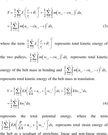
It can be seen by comparing Figs. 13 and 14 that the first natural frequency is split into two with the second frequency becoming significantly higher due to ground stiffness. Mode shapes for this study are shown in Fig. 15. Other natural frequencies and mode shapes are not shown, since the effect of ground stiffness is not significant. Only four basis functions per span are considered here, but more basis functions are required for higher natural frequencies. Other parameters in the study are k=10, 0s= , γ=400 with

1 2 1

P=P = .

(9)

(a) s=0

(b) s=0

Figure 15. First mode for bottom span.

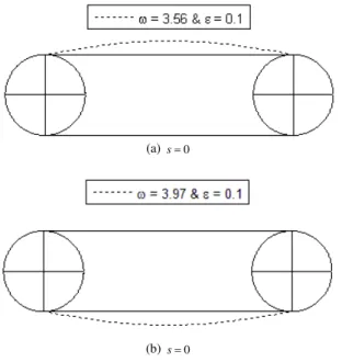
Figure 16 shows that there is an increase in the natural frequencies with ground stiffness primarily in the lower modes. It is also observed from Figs. 16 and 17 that for lower speeds the frequencies do not vary much, but for higher speeds the first three frequencies decrease, while the fourth increases. This can be interpreted with mode shapes (see Fig. 18). At higher speeds, there is a contribution from the other coefficients ai of the corresponding

span for the fourth eigenvector. The change in mode shape is observed clearly from the third mode onwards, where the amplitude level of corresponding shape started decreasing due to the presence of other non-zero coefficients ai, while the first and second modes

are strictly sine waves, which are not shown here. The other parameters used are ε=0.1, 10k= , 400γ= with P1=P2=1.

Figure 16. Natural frequency variation with belt speed for ε = 0.1 and k = 10.

Figure 17. Natural frequency variation with belt speed for ε = 0.1 and k = 0.

Conclusions

A mathematical model of a pulley-belt system with ground stiffness is presented. Equilibrium analysis is performed, which includes a numerical solution to determine the span equilibrium configuration. Dynamic analysis, which consists of the extended operator formulation, the Galerkin’s discretization and the eigenvalue problem solution, is conducted and free vibration about steady motions is examined. The formulation is validated with the results of Kong and Parker (2003). The effect of various parameters on the equilibrium and free vibration behavior has been examined. The major conclusions are summarized in the following paragraph.

As bending stiffness varies, there is a considerable decrease in equilibrium deflections due to ground stiffness, when it is larger than bending stiffness and this effect is greater for higher values of bending stiffness. The effect of ground stiffness on the equilibrium deflections is considerable with static span tension variation, while it is much more significant with variation of speed and longitudinal stiffness. With bending stiffness variation, only first natural frequency is increased due to ground stiffness. There is an increase in the natural frequencies with ground stiffness primarily in the lower modes, as speed varies. For lower speeds the frequencies do not vary much, but for higher speeds the first three frequencies decrease while the fourth increases. For the fourth eigenvector there is a considerable contribution from the other coefficients ai of the

(10)

(a) ε=0.1

(b) ε =0.1

(c) ε=0.1

(d) ε =0.1

Figure 18. Fourth mode for upper curve (bottom span).

References

Abrate, S., 1992, “Vibrations of belts and belt drives”, Mechanisms and

Machine Theory, Vol. 27, No. 6, pp. 645-659.

Beikmann, R.S., 1992 “Static and Dynamic Behavior of Serpentine Belt Drive Systems: Theory and Experiments”, Ph.D. dissertation, The University of Michigan, Ann Arbor, Michigan.

Beikmann, R.S., Perkins, N.C., and Ulsoy, A.G., 1996a, “Design and analysis of automotive serpentine belt drive systems for steady state performance”, ASME Journal of Mechanical Design, Vol. 119, pp. 162-168.

Beikmann, R.S., Perkins, N.C., and Ulsoy, A.G., 1996b, “Free vibration of serpentine belt drive systems”, ASME Journal of Vibration and Acoustics, Vol. 118, pp. 406-413.

Bhat, R.B., Xistris, G.D., and Sankar, T.S., 1982, “Dynamic behavior of a moving belt supported on elastic foundation”, ASME Journal of

Mechanical Design, Vol. 104, pp. 143-147.

Hawker, L.E., 1991, “A Vibration Analysis of Automotive Serpentine Accessory Drive Systems”, Ph.D. dissertation, University of Windsor, Ontario, Canada.

Jha, R.K., and Parker, R.G., 2000, “Spatial discretization of axially moving media vibration problems”, ASME Journal of Vibration and

Acoustics, Vol. 122, pp. 290-294.

Kong, L., and Parker, R.G., 2003, “Equilibrium and belt-pulley vibration coupling in serpentine belt drives”, ASME Journal of Applied

Mechanics, Vol. 70, pp. 739-750.

Kong, L., and Parker, R. G., 2004, “Coupled belt-pulley vibration in serpentine drives with belt bending stiffness”, ASME Journal of Applied

Mechanics, Vol. 71, pp. 109-119.

Meirovitch, L., 1967, “Analytical Methods in Vibrations”, The Macmillan Company, New York.

Meirovitch, L., 1974, “A new method of solution of the eigenvalue problem for gyroscopic systems”, AIAA Journal, Vol. 12, No. 10, pp. 1337-1342.

Mote, C.D., Jr., 1972, “Dynamic stability of axially moving materials”,

The Shock and Vibration Digest, Vol. 4, No. 4, pp. 2-11.

Oz, H.R., Pakdemirli, M., and Ozkaya, E., 1998, “Transition behaviour from string to beam for an axially accelerating material”, Journal of Sound

and Vibration, Vol. 215, No. 3, pp. 571-576.

Ozkaya, E., and Pakdemirli, M., 2000, “Vibrations of an axially accelerating beam with small flexural stiffness”, Journal of Sound and

Vibration, Vol. 234, No. 3, pp. 521-535.

Parker, R.G., 1999, “Supercritical speed stability of the trivial equilibrium of an axially-moving string on an elastic foundation”, Journal of

Sound and Vibration, Vol. 221, No. 2, pp. 205-219.

Parker, R.G., 2004, “Efficient eigensolution, dynamic response, and eigensensitivity of serpentine belt drives”, Journal of Sound and Vibration, Vol. 270, pp. 15-38.

Perkins, N.C., 1990, “Liner dynamics of a translating string on an elastic foundation”, ASME Journal of Vibration and Acoustics, Vol. 112, pp. 2-7.

Wickert, J.A., and Mote, C.D., Jr., 1988, “Current research on the vibration and stability of axially moving materials”, The Shock and Vibration

Digest, Vol. 20, No. 3, pp. 3-13.

Zhang, L., and Zu. J.W., 1999, “Modal analysis of serpentine belt drive systems”, Journal of Sound and Vibration, Vol. 222, No. 2, pp. 259-279.

Zhang, L., Zu, J.W., and Hou, Z., 2001, “Complex modal analysis of non-self-adjoint hybrid serpentine belt drive systems”, ASME Journal of