Abstract
Composite structural elements of steel-concrete began to be used only in 1960 after the development of methods and constructive dispositions that ensured the functionality of these two materials together. In order to verify the importance of the participation of the axial mode in the frequency spectrum of the free vibration problem in composite beams with deformable shear connection, several analyses for 4 different boundary conditions and stiffness connection variation were performed.
The analysis of the problem was carried out by development and computational implementation of a finite element for composite beams with partial interaction in the longitudinal direction ap-plied to the problem of free vibrations. The solutions to this problem in the literature are scarce, and project recommendations are simplified. The results show that the finite element exhibits an excellent performance compared with the analytical results and as the axial mode has a high modal contribution, despite the boundary condition and stiffness connection.
Keywords
Dynamic analysis, composite beams, deformable shear connection, Finite Elements Method, numerical analysis.
Parametric Modal Dynamic Analysis of Steel-Concrete
Composite Beams with Deformable Shear Connection
1 INTRODUCTION
Composite elements are becoming more popular in civil engineering structures, especially the com-posite elements of steel and concrete, formed by the association of profiles or steel plates with plates or linear elements of plain or reinforced concrete. The association seeks to obtain a structural ele-ment which combines the specific advantages of each material.
Steel and concrete are mechanically connected by the shear connectors. Thus, for the correct use of these structural elements it is necessary to understand the behavior of each element present in
Wanderson G. Machado a Francisco de A. Neves b João Batista M. de Sousa Jr. c
a Universidade Federal Ouro Preto, Escola de Minas, Departamento de En-genharia Civil, Ouro Preto, MG, Brasil, [email protected] b Universidade Federal Ouro Preto, Escola de Minas, Departamento de En-genharia Civil, Ouro Preto, MG, Brasil, [email protected]
c Universidade Federal do Ceará, Departamento de Engenharia Civil, Fortaleza, CE, Brasil,
http://dx.doi.org/10.1590/1679-78252981
the cross section as well as the behavior of all elements together, which is possible from the interac-tion provided by the longitudinal forces exerted by the connectors. There is a need for experimental and numerical assessments in order to provide a basis for better understanding of their behavior, and the objective of this work is to contribute in the field of numerical dynamic analysis of compo-site beams.
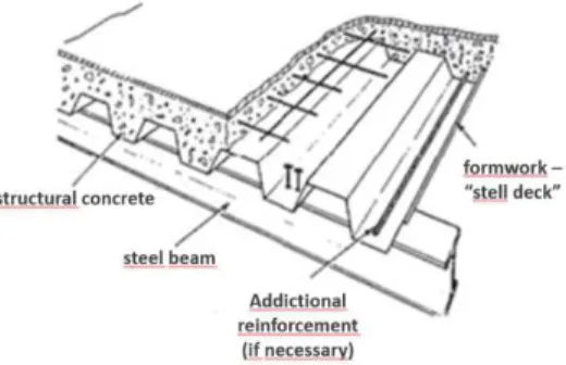
The most common steel-concrete composite structural elements are the composite column, the composite beam and the composite slab. Usually composite beams are idealized from an approxima-tion of concrete slabs connected mechanically to steel beams by shear connectors (Figure 1), since composite beam solution is adopted in most of steel buildings. It takes advantage of the presence of the concrete slab cast over the steel beam, thereby forming a composite system with superior struc-tural behavior when compared with the isolated steel beam. This improved strucstruc-tural behavior of the composite element, along with the growing use of steel structures in civil construction in Brazil has caused a significant increase in the use of this construction technique. This type of solution is also widely used when there are big spans as in bridges and industrial buildings. Some of the ad-vantages of the composite beams compared with simple beams are: high ratio span versus beam height, less deformation and a high fundamental frequency of vibration (Nie et al., 2004).
Figure 1: Composite floor shaped of composite slab associated with the steel beam.
The advantages of steel-concrete composite systems aside from those mentioned are: possibility of elimination of forms and shoring (depending on the adopted constructive sequence), reduced self-weight and volume of the structure, increased dimensional accuracy of the construction, reduced structural steel consumption, reduced protection against fire and corrosion, and increased stiffness and resistance to buckling (Queiroz et al., 2001). In composite beams one can also mention the pre-vention of buckling in the upper flange of the steel profile and buckling in the lateral side of the profile. Since they have their pre-manufactured steel elements, these systems have structural quali-ty, accuracy and execution time lower than the structural systems in which all elements are molded in place.
The numerical simulation is made by the Finite Element Method (FEM), using an element with ten degrees of freedom, as used in the work of Dall'Asta and Zona (2004a), Silva (2006) and Oliveira (2009) for static analysis, which was adapted to solve dynamic analysis problems. The ele-ment used is based on Euler-Bernoulli’s beam theory and considers the slip incorporated into its formulation.
The results for the Finite Element used in this article are compared to results obtained for ele-ments developed by others and compared with analytical results (exact), in order to validate the efficiency of this element for the dynamic analysis of the composite beam problem.
In addition to the transverse mode shapes, this work aims to detect modes of axial vibration by checking their participation in the results obtained for the composite beam problem with partial interaction, as the connection stiffness is modified, i.e, longitudinal interaction is altered.
2 PARTIAL INTERACTION
Materials have natural adhesion, however, although it may be high, it is often not considered in the calculation of a structure due to its low reliability. For this reason, it becomes necessary to use ele-ments, as shear connectors or other mechanical resources, in order to promote more interaction between interfaces of constituent materials of the composite element.
Shear connectors functions by absorbing the shearing efforts induced in the materials interface, providing a connection in the interface of both materials, decreasing longitudinal slip of the material (slip at the interface) and also vertical separation of the materials interface (displacement vertical).
The interaction in the interface can be partial or total. Under total interaction there is no slip in the interface or this slip is so small that can be neglected in the analysis, whereas in partial in-teraction, the slip has an important contribution to global behavior of the composite system or the structure in which the element is inserted, with effects on the analysis and design.
In this article, all analyses will be made considering the partial interaction at the materials in-terface of the steel-concrete composite beam. The partial interaction will be considered only in the horizontal direction, and total interaction is considered in the vertical direction, i.e., there is no vertical separation of the elements in the interface (uplift). Salari and Spacone (2001) reported that the reason of not considering the vertical separation is due to the absence of experimental evidence in composite beams analyses that prove its importance in the response.
There are several different devices that can be employed as shear connectors. A review of differ-ent types of connectors along with their main characteristics was presdiffer-ented by Shariati et al. (2012). Among these one can cite the headed stud bolt (Lee et al. 2005), the angle and channel connectors (Shariati et al., 2013, Maleki and Bagheri, 2008, 2008a), the various types of perfobond connectors (Vellasco et al. 2007) and many recently proposed schemes (Shariati et al.,2012). The most fre-quently employed shear connectors in buildings are the headed stud bolts. In terms of dynamic analysis the connectors play an important role on the energy dissipation that takes place after dy-namic excitations which may occur due to events such as seismic actions.
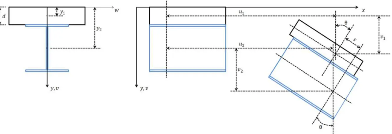
Figure 2: Displacements on the composite beam with incorporated slip.
According to Figure 2, the partial interaction on steel-concrete interface causes a slip in the in-terface given by:
2 1
( )
s x =u -u +hq (1)
where h is the distance between geometric centers of the cross sections corresponding to the constit-uent materials of the composite beam.
3 FREE VIBRATIONS PROBLEM
In the analysis of free vibration of a structure, there are two very important dynamic characteristics to be determined: natural frequencies and natural mode shapes.
Excluding damping, the equation of motion is given by:
Md + Kd = 0 (2)
To find the natural frequencies and mode shapes, one should solve the classic eigenproblem:
2
( )
j n
w j
K - M f = 0 (3)
where wnj are the natural frequencies (eigenvalues) for each degree of freedom, obtained by the
fol-lowing polynomial equation:
2
det | ( ) |
j n w
K - M = 0 (4)
Mode shapes (eigenvectors) are obtained by substituting the values found in Equation 4 into Equation 3.
Normalization of eigenvectors leads to:
T
f f
f f
= j
j
j M j
wherefjis the eigenvector before normalization, and fjis the normalized eigen vector. The normalized modal matrix consisting of N mode shapes is given by:
1,1 1,N
N,1 N,N
F
F
F
F
F
é
. . .
ù
ê
ú
ê
.
. . .
.
ú
ê
ú
ê
.
. . .
.
ú
= ê
ú
ê
.
. . .
.
ú
ê
ú
ê
. . .
ú
ê
ú
ë
û
(6)
4 FINITE ELEMENT FORMULATION FOR COMPOSITE BEAMS
Numerical solution via the finite element method for composite beam problems has raised he inter-est of many researchers around the world, and several works using elements of this type may be found, such as Oven et al. (1997), Faella et al. (2002), Salari and Spacone (2001) and Liang et al. (2004).
The solution for composite beam problem by using numerical methods becomes very interesting once these methods can be applied to all types of beams, including the more complex cases, for which there is no analytical solution. Numerical solution for the problem converges to analytic solu-tion as the finite element mesh is refined.
4.1 Finite Element
The finite element used is composed of 10 degrees of freedom, with relative slide on the interface of its materials, named after Machado (2012) as "SLIP10DOF" as shown in Figure 3.
Figure 3: Degrees of freedom of the finite element “SLIP10DOF”.
Where ui, j, vi e θi are axial displacements, vertical displacements and rotation, respectively, and the index i determines the type of material, where 1 corresponds to concrete and 2 corresponds to steel.
functions to ensure the continuity of the vertical and axial displacements, and rotations in the ends of the elements, where the latter are considered the same as those derived from the transverse dis-placements. To ensure these requirements, it must have at least a third degree polynomial for the transverse displacement, and at least linear for axial displacements. Presented below are the stiff-ness and mass matrices of the element.
4.2 Stiffness Matrix of the Element “SLIP10DOF”
First, the notation used for the deduction of the problem formulation is shown in Figure 4.
Figure 4: Distances to the axis of the element "SLIP10DOF".
The values y1 and y2 are respectively the distances from the x axis to the center of the concrete and steel sections, h is the distance between the centers of the sections, and b and t are respectively the distances of the centers of the concrete and steel sections to the contact interface of the materi-als and the super index 0 (zero) implies values at the reference axis.
Machado (2012) presents the expressions related to axial displacements u1 and u2, vertical dis-placement v e slip s identified in Figure 2.
According to kinematics, the expressions related to u1, u2, v and s are given respectively by:
0 0
1 1 ( 1) 1 ( ) ( 1) ( )
u =u - y-y q =u x - y-y qx (7)
0 0
2 2 ( 2) 2 ( ) ( 2) ( )
u =u - y-y q =u x - y-y qx (8)
0
( , ) ( )
v x y =v x (9)
0 0
2 2 1 1 2 1
( ) ( , ) ( , ) ( ) ( ) ( )
s x =u x y - -t u x y -b =u x -u x +h xq (10)
The total strain energy is given by the sum of the parts of axial strain of materials 1 and 2 to the portion of strain due to slip.
² ²
2 2
V V
Ee Fs
After calculating axial strain ε1 and ε2 for materials 1 and 2, concrete and steel, such as partial derivatives of the axial displacements u1 and u2, respectively, and replacing in Equation 11, the element strain energy in matrix form is obtained, incorporating the slip straining portions, given by:
0
1 1 1 1 1
0
2 2 2 2
0 0 2
1 2
1 1 2 2 1 1 2 2
0 0 0 0 0 1 0 2
0 0 0
L
E A E S
E A E S
U k s dx
E S E S E I E I k
F s
ì ü
é ù ïï ïï
ê ú ï ï
ê ú ïïï ïïï
ê ú
= ê + ú ï ïí ý
ê ú ïï ïï
ê ú ï ï
ê ú ï ï
ë û ïî ïþ
ò
e e
e e (12)
where k is the connection stiffness.
In a more compact form, equation 12 can be given by:
0 1 ( ) ( ) 2 L T
U =
ò
ex Dex dx (13)where ε is the strain vector written as:
0 0 1 1 0 0 2 2 0 0 0 0 ( ) ² 0 0 ² 1 1 d dx d u
dx u u x
d k v dx s d h dx e e e é ù ê ú ê ú ì ü
ï ï ê ú
ï ï ê úìï üï
ï ï ï ï
ï ï ê ú ï ï
ï ï
ï ï ê úï ï
=íï ýï= ê - úíï ýï=
ï ï ê úï ï
ï ï ê úï ï
ï ï ïî ïþ
ï ï ê ú
ï ï
î þ ê ú
-ê ú
ë û
(x) (14)
and D is the matrix composed of physical and geometrical properties, where F is the force along the interaction.
The nodal displacements vector d of the finite element shown earlier in Figure 3 is:
1 2
T T T T
u u v
=
d d d d (15)
where
1 u
d is the axial displacement vector of element 1,
2 u
d is the axial displacement vector of
ele-ment 2, and dv the vertical displacement vector and rotations of elements 1 and 2, given by:
1 1,1 1,2 1,3 T
u = u u u
d (16)
2 2,1 2,2 2,3 T
u = u u u
d (17)
1 1 2 2
T
v = v v
d q q (18)
where the superscript T involves the transposition of the vector or matrix.
Discretizing by MEF, the axial and vertical displacements of the element, defined by the inter-polation functions in the x coordinate, are respectively given by:
1 1 u( ) u
u =N xd (19)
2 2 u( ) u
u = N x d (20)
( ) v v
v =N xd (21)
where Nu and Nv are interpolation functions in the x coordinate, and integration ends are 0 (zero) and L. These interpolation functions will be determined later for a general coordinate ξ.
In matrix form:
1
2
`
( )
( ) ( )
( ) u u
u u
v v
x
x x
x
ì ü
é ù ïï ïï
ê ú ï ï
ï ï
ê ú
= = ê ú ï ïí ý
ê ú ïï ïï
ê ú ï ï
ë û î þ
d
N 0 0
u Nd 0 N 0 d
0 0 N d
(22)
After substituting the equation 22 in equation 14, the strain vector ε(x) is obtained as a func-tion of the matrix which contains the derivatives of interpolafunc-tion funcfunc-tions.
( )x ( )x
e =B d (23)
Substituting equation 23 into equation 12 or 13, in compact form, the strain energy is obtained, in terms of stiffness matrix,
1
( ) 2
T
U = d K x d (24)
with the stiffness matrix given by:
0
( ) ( ) ( )
L T
x =
ò
x x dxK B DB (25)
and B is a matrix obtained from the derivative of the interpolation matrix given by:
, ,
, , ( )
u x u x
u xx
u u v x
x
h
é ù
ê ú
ê ú
ê ú
= ê - ú
ê ú
ê ú
ê ú
ë û
N 0 0
0 N 0
B
0 0 N
N N N
(26)
1 2 1 ( 1) 2 1 ² 1 ( 1) 2
T T T
u u u
é ù
ê - ú
ê ú
ê ú
= = = ê - ú
ê ú
ê + ú
ê ú
ê ú
ë û
N N N
x x x x x (27) 3 2 3 3 2 3
1 3 1
2 4 4
1 1 1 1
2 4 4 4 4
1 3 1
2 4 4
1 1 1 1
2 4 4 4 4
T v
L
L
é ù
ê - + ú
ê ú
ê æ ö ú
ê çç - - + ÷÷ ú
ê çè ÷ø ú
ê ú
= ê ú
ê + + ú
ê ú
ê æ öú
ê ç- - + + ÷ú
ê çç ÷÷ú
è ø
ê ú
ë û
N
x x
x x x
x x
x x x
(28)
where the coordinates of their integration ends are -1 and 1, and
2 1 x L = -x (29)
Substituting the interpolation functions at the coordinate ξ (equations 27 and 28) in the matrix B(x), the matrix B(ξ) obtained is:
, , 2 , , ( ) u u v
u u v
d dx d dx x d dx d h dx é ù ê ú ê ú ê ú ê ú ê ú ê ú
= ê æ ö ú
ê - çç ÷÷ ú
ê çè ÷ø ú
ê ú
ê ú
ê ú
ê ú
ë û
N 0 0
0 N 0
B
0 0 N
N N N
x x xx x x x x x (30) where, 2 d
dx = L
x
(31)
Therefore, the general Stiffness Matrix in function of ξ is given by:
1
1
( ) ( )T ( ) d d
dx
+
-æ ö ç ÷
= çç ÷÷
è ø
ò
K x B x DBx x x (32)
4.3 Mass Matrix of the Element “SLIP10DOF”
1 1
2 2
1 2
0
L u u v
u u v
vu vu vv
dx
é ù
ê ú
ê ú
= ê ú
ê- ú
ê ú
ë û
ò
m 0 m
M 0 m m
m m m
(33)
where
1 1 1
0
L
T u =
ò
A u udxm r N N (34)
2 2 2
0
L
T u =
ò
A u udxm r N N (35)
1 1 1 ,
0
L
T u v =
ò
S u v xdxm r N N (36)
2 2 2 ,
0
L
T u v =
ò
S u v xdxm r N N (37)
1 1 2 ,
0
L
T vu =
ò
S v x udxm r N N (38)
2 2 2 ,
0
L
T vu =
ò
S v x udxm r N N (39)
(
1 1 1 1 , ,) (
2 2 2 2 , ,)
0
L
T T T T
vv =
ò
A v v + I v x v x + A v v + I v x v x dxm r N N r N N r N N r N N (40)
where 1 1 ,T , v x v x
I
r N N is the inertia of the rotating section. If the axes are in the centroids,
1 0
u v =
m
and
1 0 vu =
m , where ρ, A, S and I are respectively the specific weight, area, static moment and inertia moment for materials 1 and 2.
Switching to the general coordinate "ξ", the mass matrix is given by:
1
1
( ) ( ) d d
dx
+
-é ù =
ò
ë ûM x M x x x (41)
where,
1 2
dx L
d d
dx
= =
5 NUMERICAL EXAMPLE
The example was based on Xu and Wu (2007) and is intended to determine two important parame-ters for composite beams dynamic analysis, natural frequencies and mode shapes with partial inter-action, noting the influence of connection stiffness in these parameters.
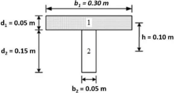
The example to be solved is a composite beam, whose cross section is shown in Figure 5, and the which geometric and material properties of the cross section are as follows: L=4m, h=0.1m (dis-tance between centers of gravity of the materials 1 and 2), E1=12GPa, E2=8GPa, A1=0.015m²,
A2=0.0075m², I1=3.125x10⁻⁶m4, I2=1.40625x10⁻⁴m4, m1=36kg/m e m2=3.75kg/m.
Figure 5: Composite beam.
Analysis of the parameters will be done for different connection stiffnesses, Ks, aiming to verify the influence of connection stiffness variation on the mode shape analysis. Therefore, for each analy-sis, the connection stiffness will assume the values of: 50MPa, 1 MPa, 0.1MPa and 0.01MPa.
Xu and Wu (2007) treated the same example for different boundary conditions. They have de-veloped and solved analytically (exactly) the differential equations of the problem. Their analysis followed four scenarios: the first considered strain due to shear and rotation inertia. The second hypothesis considered only strain due to shear; the third considered only rotation inertia and, in the final analysis, neither of the two factors was considered.
Due to the assumptions made in the formulation of the finite element, strains due to shear are not considered in this work, but rotation inertia will be considered. So as in Xu and Wu (2007), analyses will be made to the four boundary conditions: simply supported, clamped - supported clamped - free and clamped - clamped.
5.1 Simply Supported Beam
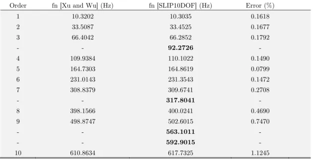
Considering Ks = 50MPa, natural frequencies are determined and compared with the analytical results obtained by Xu and Wu (2007). Results will be obtained for a 15 mesh element since this quantity of finite elements has proved sufficient, and for fewer elements some values differed consid-erably from the exact values.
Order fn [Xu and Wu] (Hz) fn [SLIP10DOF] (Hz) Error (%)
1 10.3202 10.3035 0.1618
2 33.5087 33.4525 0.1677
3 66.4042 66.2852 0.1792
- - 92.2726 -
4 109.9384 110.1022 0.1490
5 164.7303 164.8619 0.0799
6 231.0143 231.3543 0.1472
7 308.8379 309.6741 0.2708
- - 317.8041 -
8 398.1566 400.0241 0.4690
9 498.8747 502.6015 0.7470
- - 563.1011 -
- - 592.9015 -
10 610.8634 617.7325 1.1245
Table 1: Natural frequencies for simply supported beam.
The obtained values indicate a good approximation to the values found by Xu and Wu (2007) showing that the finite element of ten degrees of freedom, SLIP10DOF, developed in Machado (2012), have good accuracy, since Xu and Wu (2007) values are exact (analytical), thus proving the efficiency of the element used.
In this work, as well as Machado (2012), frequencies corresponding to predominantly axial dis-placements were also determined, thereby resulting in axial shape modes of the beam. Axial fre-quency values are highlighted in Table 1, which are not determined by Xu and Wu (2007) in their analysis, since these authors considered only the transverse vibrations of the beam. On Table 1, one can see that for the simply supported beam, 4th natural frequency implies an axial mode shape, showing how important is the consideration of the axial mode.
In order to evaluate the influence of connection stiffness on dynamic characteristics (natural frequencies and mode shapes), a variation in the values of connection stiffness will be conducted, as shown in Table 2:
By reducing connection stiffness, or reducing the interaction at the interface, the axial mode shapes become more prevalent, coming to appear as the 1st mode shape when the connection stiff-ness value is in the order of 0.01Mpa. But a better analysis of the participation of these axial modes will be performed using the graphs contained in figures 6-9.
The axial mode found in this work led to evaluate participation (in percentage) of mode shapes in the results obtained, especially the participation of axial mode shape. For the numerical analysis, 15 SLIP10DOF elements were used, each element has 10 degrees of freedom in local system (Figure 3).
Or-der
fn [SLIP10DOF] for 50MPa (Hz)
fn [SLIP10DOF] for 1MPa (Hz)
fn [SLIP10DOF] for 0.1MPa (Hz)
fn [SLIP10DOF] for 0.01MPa (Hz)
1 10.3035 6.3367 6.0624 2.7087
2 33.4525 24.4315 8.5309 6.0333
3 66.2852 25.9699 24.1436 24.1143
4 92.2726 54.5420 54.2513 54.2221
5 110.1022 96.6460 96.3547 96.3254
6 164.8619 150.7205 150.4292 150.4000
7 231.3543 216.7654 212.4280 211.4024
8 309.6741 222.5015 216.4745 216.4454
9 317.8041 286.8255 285.6492 285.5334
10 400.0241 294.8245 294.5343 294.5053
11 502.6015 385.0064 384.7172 384.6883
12 563.1011 487.5040 487.2160 487.1872
13 592.9015 571.6813 571.1165 571.0588
14 617.7325 602.6086 602.3222 602.2935
Table 2: Natural frequencies for simply supported beam varying with the connection stiffness.
In order to better evaluate the influence of these axial modes in response for the problem, graphs below show the participation of each mode shape (in percentage). For this purpose, the ef-fective mass of each mode shape were calculated and divided by the total mass of the system, find-ing the participation of each mode shape.
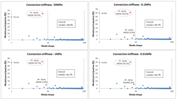
Analyzing the graphs of Figure 6, one can see that the first mode shapes are responsible for al-most all of the effective mass of the structure, so in an analysis to calculate the dynamic response via method of modal superposition, the contribution of these modes would be enough to obtaining accurate results. In order to illustrate, an analysis is made considering the first 10 modes, where they contribute in more than 96% of the system mass.
The participation values of AXIAL modes are highlighted, where it is clear that its modal par-ticipation is high even when the connection stiffness is high (41.1% for a stiffness of the 50MPa), and it is not necessary to decrease connection stiffness for it to play a crucial role. However, one notices that other axial modes appear as the connection stiffness is reduced, although with lower participation, but either way, showing the important role of these axial mode shapes.
5.2 Other Support Conditions
In order to verify the influence of support conditions with respect to modal participation and im-portance of axial mode when it varies the connection stiffness, several graphics for different stiffness are presented below.
5.2.1 Clamped-Free Beam
5.2.2 Clamped-Supported Beam
Figure 8: Mode shapes participation for different values of connection stiffness (clamped-supported beam).
5.2.3 Clamped-Clamped Beam
Figure 9: Mode shapes participation for different values of connection stiffness (clamped -clamped beam).
it reduces the connection stiffness, more influences of axial modes arise. In fact, it is clear that there is a reduction in the order of appearance of axial mode when it reduces the connection stiffness of 50 to 1 MPa, and statistically no influence is perceived when it reduces to 0.01MPa.
5.3 Fundamental Frequency / Axial Frequency x Boundary Conditions x Connection Stiffness
Following, the influence of different boundary conditions on the fundamental frequency of vibration (Figure 10) will be evaluated, as well as the 1st axial frequency (Figure 11). The boundary condi-tions are analyzed: simply supported, clamped-free, clamped-supported and clamped-clamped, and the analysis made for a stiffness range of 0.001Mpa to 500Mpa.
Figure 10: Assessment of the influence of different boundary conditions and stiffness on the Fundamental Frequency.
Figure 11: Assessment of the influence of different boundary conditions and stiffness on the 1st Axial Frequency.
About Figure 11, it can be said that the variation of the 1st frequency of axial vibration in rela-tion to boundary condirela-tions and variarela-tion of stiffness is too small for the clamped-supported beam, clamped-free and clamped-clamped beam. However, for the simply supported condition, it is clear that from the 0.1MPa stiffness, there is a wide variation with the stiffness variation, showing that the axial frequency has greater influence for simply supported beams, as it is easily perceived in the analysis of figures 6-9, where it was shown the appearance of axial modes for different boundary conditions and it was verified that for the simply supported condition, 1st axial mode emerged as a fundamental frequency for the stiffness of 0.01Mpa (Figure 6). It is also observed that for clamped-free and clamped-supported conditions, the values of the first axial frequencies for the different stiffness are practically equal.
6 CONCLUSIONS
SLIP10DOF element developed and implemented by Machado (2012) to composite beams, consider-ing the partial interaction applied to the problem of free vibrations, showed an excellent perfor-mance when compared with the analytical results and other numerical approaches available in the literature.
With the variation of the connection stiffness and boundary conditions (support), it can be seen clearly how these boundary conditions influence the axial vibration modes. One sees clearly the importance of considering the axial mode, since for all analyses with different boundary conditions and variation in connection stiffness, modal contribution of this mode varies approximately 35-44%, particularly for simply supported beams, where there is a contribution of around 44% regardless of the connection stiffness value. Also for the simply supported case, one can note that as the connec-tion stiffness reduces, the order corresponding to the appearance of axial mode decreases, so that for stiffness equals to 0.01MPa, axial mode frequency appears as fundamental vibration. This was not observed for the other boundary conditions.
Another point worth mentioning is the emergence of other axial modes, of a higher order, when connection stiffness reduces. It appears that first 10 mode shapes are responsible for modal contri-bution of 86-97% when considering all boundary conditions versus the variation of the connection stiffness. Moreover, the axial modes for all variations of boundary conditions and connection stiff-ness contributed 40-48% in the modal participation.
It can be conclude therefore that the axial modes are important contributions to the vibration system and must be considered in the calculation of response to a dynamic analysis to obtain good results.
The variation of the first axial mode frequency is negligible for boundary conditions other than the simply-supported case, for which already for very low values of the shear connection (0,01 MPa) displays an important variation with the connection stiffness.
have a low degree of partial shear connection (low degree of interaction). This is in accordance with the researches conducted by Bursi and Gramola (2000) and Bursi et al. (2005).
Acknowledgments
The authors thank CNPq, CAPES, FAPEMIG and UFOP, for their support for this work.
References
Bursi, O.S., Gramola, G. (2000). Behaviour of composite substructures with full and partial shear connection under quasi-static cyclic and pseudo-dynamic displacements. Materials and Structures/Materiaux et Constructions, 33 (3), 154-163, dx.doi.org/10.1007/BF02479409.
Bursi, O.S., Sunb, F.-F., Postal, S. (2005). Non-linear analysis of steel–concrete composite frames with full and par-tial shear connection subjected to seismic loads. Journal of Constructional Steel Research, 61 (1), 67–92, dx.doi.org/10.1016/j.jcsr.2004.06.002.
Dall'Asta, A., Zona, A. (2004a). Slip Locking in Finite Elements for Composite Beams with Deformable Shear Con-nection. Finite Elements in Analysis and Design, 40 (13-14), 1907-1930, dx.doi.org/10.1016/j.finel.2004.01.007. Eurocode 4 (2004). Design of composite structures (ENV 1994)’ Part 1-1/1992 General rules and rules for buildings”, CEN Publications, Brussels, Belgium.
Faella, C., Martinelli, E., Nigro, E. (2002). Steel and Concrete Composite Beam with Flexible Shear Connection: “Exact” Analytical Expression of the Stiffness Matrix and Applications. Computer & Structures, 80 (11),1001-09, dx.doi.org/10.1016/S0045-7949(02)00038-X
Lee, P., Shim, C., Chang, S. (2005). Static and fatigue behavior of large stud shear connectors for steel-concrete composite bridges. Journal of Constructional Steel Research, 61(9), 1270-1285, dx.doi.org/10.1016/j.jcsr.2005.01.007. Liang, Q.Q., Uy, B., Bradford, M.A., Ronagh, H.R. (2004). Ultimate Strength of Continuous Composite Beams in Combined Bending and Shear. Journal of Constructional Steel Research, 60(8), 1109-28, dx.doi.org/10.1016/j.jcsr.2003.12.001.
Machado, W.G. (2012). Análise Dinâmica de Vigas Mistas com Interação Parcial (Dynamic Analysis of Composite Beams with Partial Interaction), MSc Dissertation, Department of Civil Engineering, Escola de Minas, Federal Uni-versity of Ouro Preto (in Portuguese). Available at www.propec.ufop.br.
Maleki, S., Bagheri, S. (2008) Behavior of channel shear connectors, Part I: Experimental study, Journal of Con-structional Steel Research, 64(12), 1333-1340, dx.doi.org/10.1016/j.jcsr.2008.01.010.
Maleki, S., Bagheri, S. (2008a). Behavior of channel shear connectors, Part II: Analytical study Journal of Construc-tional Steel Research, 64(12), 1341-1348, dx.doi.org/10.1016/j.jcsr.2008.01.006.
Maleki, S., Mahoutian, M. (2009) Experimental and analytical study on channel shear connectors in fiber-reinforced concrete, Journal of Constructional Steel Research, 65 (8-9), 1787-1793, dx.doi.org/10.1016/j.jcsr.2009.04.008. Nie, J.F., Cai, C.S. (2004). Stiffiness and Deflection of Steel-Concrete Composite Beams under Negative Bending. Journal of Structural Engineering, 130 (11), 1842 -51, dx.doi.org/10.1061/(ASCE)0733-944.
Oehlers, D.J., Bradford, M.A. (1999). Elementary Behaviour of Composite Steel ans Concrete Structural Members. Oxford: Butterworth Heinemann.
Oliveira, C.E. (2009). Análise Não-Linear Geométrica de Vigas-Colunas com Interação Parcial (Nonlinear Analysis of Geometric Beam-columns with Partial Interaction), MSc Dissertation, Department of Civil Engineering, Escola de Minas, Federal University of Ouro Preto (in Portuguese). Available at www.propec.ufop.br.
Queiroz, G., Pimenta, R.J., Da Mata, L.A. (2001). Elementos das Estruturas Mistas Aço-Concreto (Elements of Composite Structures Steel-Concrete). Belo Horizonte: O Lutador (in Portuguese).
Salari, M.R., Spacone, E. (2001). Finite Element Formulations of One-Dimensional Elements with Bond-slip. Eng. Struct., 23 (7), 815–26, dx.doi.org/10.1016/S0141-0296(00)00094-8.
Shariati, A., Sulong, N.H.R., Suhatril, M., Shariati, M. (2012). Various types of shear connectors in composite struc-tures: A review. International Journal of Physical Sciences ,7(22), 2876-2890, dx.doi.org/10.13140/RG.2.1.1903.0563 Shariati, M., Sulong, N.H.R., Suhatril, M., Shariati, A., Arabnejad Khanouki, M.M., Sinaei, H. (2013) Comparison of behaviour between channel and angle shear connectors under monotonic and fully reversed cyclic loading, Construc-tion and Building Materials, 38, 582-593, dx.doi.org/10.1016/j.conbuildmat.2012.07.050.
Vellasco, P., De Andrade, S., Ferreira, L., De Lima, L. (2007). Semi-rigid composite frames with perfobond and T-rib connectors Part 1: Full scale tests. Journal of Constructional Steel Research, 63 (2), 263-279, dx.doi.org/10.1016/j.jcsr.2006.04.011
Xu, R., Wu, Y. (2007). Static, dynamic and buckling analysis of partial interaction composite members using Timo-shenko’s beam theory. International Journal of Mechanical Sciences, 49 (10), 1139–55, dx.doi.org/10.1016/j.ijmecsci.2007.02.006.
APPENDIX
Analytical Arrays (Element "SLIP 10DOF")
As the design for the stiffness, mass and damping matrices for "SLIP10DOF" element was intro-duced, the analytical matrices are presented below.
Stiffness matrix is composed of two parts (due to the strain and due to the slip), as described in Equation 11.
According to Machado (2012), the portion of the stiffness matrix due to strain (ε1 and ε2), are given respectively by:
1 1 1 1 1 1
1 1 1 1 1 1
1 1 1 1 1 1
,1
1 1 1 1 1 1 1 1
3 2 3 2
1 1 1 1 1 1 1 1
2 2
7 8
0 0 0 0 0 0 0
3 3 3
8 16 8
0 0 0 0 0 0 0
3 3 3
8 7
0 0 0 0 0 0 0
3 3 3
0 0 0 0 0 0 0 0 0 0
0 0 0 0 0 0 0 0 0 0
0 0 0 0 0 0 0 0 0 0
12 6 12 6
0 0 0 0 0 0
6 4 6 2
0 0 0 0 0 0
1
0 0 0 0 0 0
E A E A E A
L L L
E A E A E A
L L L
E A E A E A
L L L
E I E I E I E I
L L L L
E I E I E I E I
L L L L e -- -= -K
1 1 1 1 1 1 1 1
3 2 3 2
1 1 1 1 1 1 1 1
2 2
2 6 12 6
6 2 6 4
0 0 0 0 0 0
E I E I E I E I
L L L L
E I E I E I E I
L L L L é ù ê ú ê ú ê ú ê ú ê ú ê ú ê ú ê ú ê ú ê ú ê ú ê ú ê ú ê ú ê ú ê ú ê ú ê ú ê ú ê ú ê ú ê ú ê ú
ê - - ú
ê ú
ê ú
ê ú
ê - ú
ê ú
ê ú
ë û
1 1 1 1 1 1
1 1 1 1 1 1
1 1 1 1 1 1
,1
1 1 1 1 1 1 1 1
3 2 3 2
1 1 1 1 1 1 1 1
2 2
0 0 0 0 0 0 0 0 0 0
0 0 0 0 0 0 0 0 0 0
0 0 0 0 0 0 0 0 0 0
7 8
0 0 0 0 0 0 0
3 3 3
8 16 8
0 0 0 0 0 0 0
3 3 3
8 7
0 0 0 0 0 0 0
3 3 3
12 6 12 6
0 0 0 0 0 0
6 4 6 2
0 0 0 0 0 0
1
0 0 0 0 0 0
E A E A E A
L L L
E A E A E A
L L L
E A E A E A
L L L
E I E I E I E I
L L L L
E I E I E I E I
L L L L e -- -= -K
1 1 1 1 1 1 1 1
3 2 3 2
1 1 1 1 1 1 1 1
2 2
2 6 12 6
6 2 6 4
0 0 0 0 0 0
E I E I E I E I
L L L L
E I E I E I E I
L L L L é ù ê ú ê ú ê ú ê ú ê ú ê ú ê ú ê ú ê ú ê ú ê ú ê ú ê ú ê ú ê ú ê ú ê ú ê ú ê ú ê ú ê ú ê ú ê ú
ê - - ú
ê ú
ê ú
ê ú
ê - ú
ê ú
ê ú
ë û
(44)
where the stiffness matrix total due to deformation, Kε, is given by the sum of Equations 43 and 44. The portion of the stiffness matrix due to slip, Ks (Machado, 2012) is given by:
(
) (
) (
)
,1 ,1 ,2
,1 ,1 ,2
,2 ,2 ,3
s s s
s s s s
T T T
s s s
K K K
K K K K
K K K
é ù
-ê ú
ê ú
ê ú
= -ê - ú
ê - ú
ê ú
ë û
(45)
where Ks,1, Ks,2 and Ks,3 were determined only to simplify Equation 45, therefore:
,1 2
15 15 30
8
15 15 15
2
30 15 15
s
FL FL FL
FL FL FL
FL FL FL
é - ù
ê ú
ê ú
ê ú
ê ú
= ê ú
ê ú
ê- ú
ê ú ê ú ë û K (46) ,2 7
10 60 10 20
4 4
5 15 5 15
7
10 20 10 60
s
Fh FhL Fh FhL
Fh FhL Fh FhL
Fh FhL Fh FhL
é - ù
ê - ú
ê ú
ê ú
ê ú
= ê - ú
ê ú
ê - ú
ê - ú
ê ú
ë û
,3
6 ² ² 6 ² ²
5 10 5 10
² 2 ² ² ²
10 15 10 30
6 ² ² 6 ² ²
5 10 5 10
² ² ² 2 ²
10 30 10 15
s
Fh Fh Fh Fh
L L
Fh Fh L Fh Fh L
Fh Fh Fh Fh
L L
Fh Fh L Fh Fh L
é ù
ê - ú
ê ú
ê ú
ê - - ú
ê ú
ê ú
= ê ú
ê- - - ú
ê ú
ê ú
ê - - ú
ê ú
ë û
K (48)
Thus the stiffness matrix element (K) is given by the sum of the parts, that is, the sum of Equations 43-45. The mass matrix(M) is given by Equation 41, where their mass portions are given by:
1 1 1 1 1 1
1 1 1 1 1 1
1
1 1 1 1 1 1
2
15 15 30
8
15 15 15
2
30 15 15
u
A L A L A L
A L A L A L
A L A L A L
é - ù
ê ú
ê ú
ê ú
ê ú
= ê ú
ê ú
ê- ú
ê ú
ê ú
ë û
m
r r r
r r r
r r r
(49)
2 2 2 2 2 2
2 2 2 2 2 2
2
2 2 2 2 2 2
2
15 15 30
8
15 15 15
2
30 15 15
u
A L A L A L
A L A L A L
A L A L A L
é - ù
ê ú
ê ú
ê ú
ê ú
= ê ú
ê ú
ê- ú
ê ú
ê ú
ë û
m
r r r
r r r
r r r
(50)
1
1 1 1 1 1 1 1 1
1 1 1 1 1 1 1 1
1 1 1 1 1 1 1 1
7
10 60 10 20
4 4
5 15 5 15
7
10 20 10 60
u v
S S L S S L
S S L S S L
S S L S S L
é ù
ê- - ú
ê ú
ê ú
ê ú
= -ê - - ú
ê ú
ê ú
ê- - ú
ê ú
ë û
m
r r r r
r r r r
r r r r
(51)
2
2 2 2 2 2 2 2 2
2 2 2 2 2 2 2 2
2 2 2 2 2 2 2 2
7
10 60 10 20
4 4
5 15 5 15
7
10 20 10 60
u v
S S L S S L
S S L S S L
S S L S S L
é ù
ê- - ú
ê ú
ê ú
ê ú
= -ê - - ú
ê ú
ê ú
ê- - ú
ê ú
ë û
m
r r r r
r r r r
r r r r
(52)
(
)
1 1
T vu = u v
m m (53)
(
)
2 2
T vu = u v
1 2
vv = vv + vv
m m m x (55)
where,
1 1 1 1 1 1 1 1 1 1 1 1 1 1 1 1
1 1 1 1 1 1 1 1 1 1 1 1 1 1 1 1
1
1 1 1 1 1 1 1 1 1 1 1 1
13 6 11 ² 9 6 13 ²
35 5 210 10 70 5 420 10
11 ² ² 2 13 ² ²
210 10 105 15 420 10 140 30
9 6 13 ² 13 6 1
70 5 420 10 35 5
vv
A L I A L I A L I A L I
L L
A L I A L I L A L I A L I L
A L I A L I A L I
L L + + - - + + + - - -= - - + -m
r r r r r r r r
r r r r r r r r
r r r r r r 1 1 1 1
1 1 1 1 1 1 1 1 1 1 1 1 1 1 1 1
1 ²
210 10
13 ² ² 11 ² ² 2
420 10 140 30 210 10 105 15
A L I
A L I A L I L A L I A L I L
é ù ê ú ê ú ê ú ê ú ê ú ê ú ê ú
ê - ú
ê ú
ê ú
ê- + - - - - + ú
ê ú
ê ú
ë û
r r
r r r r r r r r
(56)
2 2 2 2 2 2 2 2 2 2 2 2 2 2 2 2
2 2 2 2 2 2 2 2 2 2 2 2 2 2 2 2
1
2 2 2 2 2 2 2 2 2 2 2 2
13 6 11 ² 9 6 13 ²
35 5 210 10 70 5 420 10
11 ² ² 2 13 ² ²
210 10 105 15 420 10 140 30
9 6 13 ² 13 6 1
70 5 420 10 35 5
vv
A L I A L I A L I A L I
L L
A L I A L I L A L I A L I L
A L I A L I A L I
L L + + - - + + + - - -= - - + -m
r r r r r r r r
r r r r r r r r
r r r r r r 2 2 2 2
2 2 2 2 2 2 2 2 2 2 2 2 2 2 2 2
1 ²
210 10
13 ² ² 11 ² ² 2
420 10 140 30 210 10 105 15
A L I
A L I A L I L A L I A L I L
é ù ê ú ê ú ê ú ê ú ê ú ê ú ê ú
ê - ú
ê ú ê ú ê ú - + - - - - + ê ú ê ú ë û r r
r r r r r r r r
(57)