Fabiano R. Lima
[email protected] Federal University of Santa Catarina – UFSCMechanical Engineering Department – EMC Industrial Noise Laboratory 88040-900 Florianópolis, SC, Brazil
Samir Nagi Y. Gerges
[email protected] Federal University of Santa Catarina – UFSCMechanical Engineering Department – EMC Industrial Noise Laboratory 88040-900 Florianópolis, SC, Brazil
Thiago Rodrigo L. Zmijevski
[email protected] Federal University of Santa Catarina – UFSCMechanical Engineering Department – EMC Industrial Noise Laboratory 88040-900 Florianópolis, SC, Brazil
Darlam Fábio Bender
[email protected] Federal University of Santa Catarina – UFSC Mechanical Engineering Department – EMC Industrial Noise Laboratory 88040-900 Florianópolis, SC, BrazilRafael N. Cruz Gerges
[email protected] NR Consultoria e Treinamento Ltda. Laboratório Equipamentos de Proteção Individual Rua Joe Collaço n.491 – Santa Monica 88035-200 Florianópolis, SC, BrazilUncertainty Calculation for Hearing
Protector Noise Attenuation
Measurements by REAT Method
The objective of this paper is to quantify the uncertainty of hearing protector attenuation measurements and present the metrology study necessary for the accreditation of the Industrial Noise Laboratory (LARI) at The Federal University of Santa Catarina and Individual Protection Equipment laboratory (LAEPI) of NR consultancy Ltda. – Brazil for hearing protector noise attenuation procedures using the “Real Ear Attenuation at Threshold – REAT” method of the Brazilian National Institute of Metrology Standardization and Industrial Quality – INMETRO. A model for the calculation of measurement uncertainty was developed based on the document: "Guide to expression of uncertainty in measurement" published by the International Organization for Standardization, first edition, corrected and reprinted in 1995, Geneva, Switzerland. The uncertainty of each source of error was estimated and the overall uncertainty of the hearing protector noise attenuation measurement was calculated for each 1/1 octave band frequency and the results used in the single number (NRRsf – Noise Reduction Rating for subject fit) uncertainty calculation. It was concluded that the largest uncertainty is due to the determination of the subject hearing thresholds.
Keywords: uncertainty, hearing protector, noise attenuation
Introduction
1
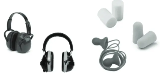
Metrology is the science of measurement and it encompasses all theoretical and practical aspects related to it. For this reason, the Metrology plays an important role in quality assurance and quality measurements. High quality measurements should be based on a well-developed procedure and supported by a standardised method to assure quality control of products. The errors of measurement can be expressed by the measurement uncertainty value. This value can be used to quantify the confidence limits of the measured results and allows comparison of measurements carried out by different laboratories and for different products (INMETRO et al., 1997). Brinkmann (1988) showed that, in spite of the different methods available for noise attenuation measurements for hearing protectors (see Fig. 1), the values for the sources of errors are still not well understood and the working groups are encountering difficulties in quantifying this measurement uncertainty. This study was developed
Paper accepted December, 2009. Technical Editor: Domingos Alves Rade
and conducted at the Vibration and Acoustics Laboratory of the Federal University of Santa Catarina, Brazil, and Individual Protection Equipment laboratory (LAEPI) of NR Consultancy Ltda., and it proposes a model for the uncertainty calculation for the hearing protector device (HPD) attenuation measurement.
Nomenclature
ANSI = American National Standards Institute; D/A = Digital/Analog;
DC = Direct Current;
HPD = Hearing Protector Device;
NRRs = Noise Reduction Rating for subject fit;
PEARPA = Program for Measurement of Hearing Protector Noise Attenuation;
REAT = Real Ear Attenuation at Threshold;
SNR84% = Single Number Rating with 84% of protection; SPL = Sound Pressure Level;
Standard uncertainty – Each one of the separate contributions to uncertainty, expressed as a standard deviation; Combined standard uncertainty – The total uncertainty resulting
of combining all uncertainty components. It is equal to the positive square root of the total variance obeying the law of propagation of uncertainty;
Expanded uncertainty – It represents the interval within the measure and value is believed to lie with a specific level of confidence. It is obtained by multiplying the combined standard uncertainty by a coverage factor. For a level of confidence that equals to 95%, the coverage factor is 2;
Mensurand – Object of measurement. Quantity under interest and submitted to the measurement process
(INMETRO et al., 1997);
Open threshold of hearing – The minimum effective sound pressure level that is capable of evoking an auditory sensation when the hearing protector under test is not worn (ANSI, 1997);
Closed threshold of hearing – The minimum effective sound pressure level that is capable of evoking an auditory sensation when the hearing protector under test is worn (ANSI, 1997).
REAT Measurements
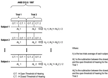
The latest standard REAT method for the measurement of the noise attenuation of hearing protectors is ANSI S12.6-1997 (ANSI, 1997) (methods A and B). The measurements are carried out in each 1/1-octave band frequency from 125 to 8000 Hz (seven bands) and the results are given in the form of an average attenuation value and a standard deviation for each frequency band. These parameters are obtained from ten attenuation measurements in case of earmuffs (ten test subjects) or twenty for earplugs (twenty test subjects). The test is repeated twice for each subject and a subject average value for these trials is calculated. Each test is composed of open and closed threshold measurements (see Fig. 2). After the calculation of this mean value for each subject, these results are used to determine the overall average and its standard deviation. As can be observed, the determination of the HPD attenuation is not a direct measurement. Instead, it is calculated from the thresholds measured for all the subjects. As will be demonstrated here, this is responsible for most of the measurement uncertainty.
Atn2 Atn1
O.T. 2 C.T. 2 O.T. 1 C.T. 1
At22 At21
O.T. 2 C.T. 2 O.T. 1 C.T. 1
At12
At11
C.T. 2 O.T. 2 C.T. 1 O.T. 1
Trial 1 Trial 2 ANSI S12.6 / 1997
Subject 1
Subject 2
Subject n
A1= ( At11+ At12 ) / 2
A2= ( At21+ At22 ) / 2
An = ( Atn1+ Atn2 ) / 2
O.T. ÆOpen Threshold of Hearing C.T. ÆClosed Threshold of Hearing
Where:
Aiis the two trials average of each subject
Ati1 is the subtraction between the closed
and the open threshold of hearing for the Trial 1
Ati2 is the subtraction between the closed
and the open threshold of hearing for the Trial 2
Figure 2. Method for hearing protector attenuation and standard deviation calculation.
Uncertainty Calculation
The general equation presented below is recommended by the “Guide to expression of uncertainty in measurements” (INMETRO et al., 1997) and shows the relation between the measurement uncertainty and the input parameters of the HPD attenuation. It can be written as:
( )
( )
( )
2 2( )
22 2
1 1
2 ⎥
⎦ ⎤ ⎢
⎣ ⎡
⋅ ∂
∂ + + ⎥ ⎦ ⎤ ⎢
⎣ ⎡
⋅ ∂
∂ + ⎥ ⎦ ⎤ ⎢
⎣ ⎡
⋅ ∂ ∂
= n
n x u x
G x
u x
G x
u x G G
u L (1)
where u(x1), u(x2), …, u(xn) are the standard uncertainties of the
input parameters for the attenuation measurement, u(G) represents the combined uncertainty of measurements and G is the mensurand. It should be clear that Eq. (1) has to be applied to the attenuation and standard deviation equations presented in Fig. 2.
Attenuation
Considering “n” test subjects, the overall average attenuation (Af) can be written as:
n
A
A
N
i i
f
∑
=
=
1(2)
(
) (
)
(
) (
)
n
OT CT OT CT ... OT CT OT CT
A
nB nB nA nA B
B A A
f 2 2
1 1 1
1 − + − + + − + −
= (3)
or
(
) (
)
(
) (
)
n
OT CT OT CT ... OT CT OT CT
Af A A B B nA nA nB nB
⋅
− + − + + − + − =
2
1 1 1
1 (4)
where CT1A is the closed threshold value for the first trial A and the first subject; OT1A is the open threshold value for the first trial A and
the first subject; CT1B is the closed threshold value for the second trial B and the first subject; OT1B is the open threshold value for the
second trial B and the first subject; CTnA is the closed threshold value for the first trial A and the n-th subject; and so on.
( )
(
)
(
)
(
)
(
)
(
)
(
)
2(
)
2(
)
22 2 1 2 1 2 1 2 1 2 2 1 2 1 2 1 2 1 2 1 2 1 2 1 2 1 ⎥⎦ ⎤ ⎢⎣ ⎡ ⋅ ⋅ + ⎥⎦ ⎤ ⎢⎣ ⎡ ⋅ ⋅ + ⎥⎦ ⎤ ⎢⎣ ⎡ ⋅ ⋅ − + + ⎥⎦ ⎤ ⎢⎣ ⎡ ⋅ ⋅ + + ⎥⎦ ⎤ ⎢⎣ ⎡ ⋅ ⋅ − + + ⎥⎦ ⎤ ⎢⎣ ⎡ ⋅ ⋅ + ⎥⎦ ⎤ ⎢⎣ ⎡ ⋅ ⋅ − + ⎥⎦ ⎤ ⎢⎣ ⎡ ⋅ ⋅ = nB nB nA nA B B A A f OT u n CT u n OT u n CT u n OT u n CT u n OT u n CT u n A u
L (5)
Equation (5) is the general expression for the calculation of the combined standard uncertainty of the HPD noise attenuation measurement. This calculation needs the uncertainty estimation of each threshold measurement (open and closed).
Standard Deviation
Similarly, the standard deviation (Sf) can be calculated by means of:
(
)
(
)
∑ ∑ = = ⋅ − − = − − = ni i f
n
i i f
f A A
n n A A S 1 2 1 2 1 1
1 (6)
or
(
) (
)
(
)
[
]
21 2 2 2 2 1 1 1 f n f f f A A A A A A n S − + + − + − ⋅ − = L (7)
where A1, A2, …, An are the average attenuations for each subject (arithmetic average of the attenuation obtained for each subject measurement).
As shown earlier, Af is a function of A1, A2, ..., An. This implies
that the derivative calculation of Eq. (7) will require a lot of mathematical work, and therefore, considering the use of the methodology presented herein and for simplicity it was considered that Af is not a function of A1, A2, ..., An and acts like a constant. An
analysis was carried out to check this assumption, which resulted in errors of less than 1%. Mathematically, the assumption can be represented by Lima (2003):
0 = ∂ ∂ i f A A (8)
Using Eqs. (1) and (7), it is possible to derive the general equation for the calculation of the combined standard uncertainty as:
( )
( )
( )
( )
2( )
22 2 2 2 1 1 2 ⎥ ⎥ ⎦ ⎤ ⎢ ⎢ ⎣ ⎡ ⋅ ∂ ∂ + ⎥ ⎦ ⎤ ⎢ ⎣ ⎡ ⋅ ∂ ∂ + + ⎥ ⎦ ⎤ ⎢ ⎣ ⎡ ⋅ ∂ ∂ + ⎥ ⎦ ⎤ ⎢ ⎣ ⎡ ⋅ ∂ ∂ = f f f n n f f f f A u A S A u A S ... A u A S A u A S S u (9)
The partial derivative calculation of Sf in terms of A1, A2, ..., An
considering the above assumption in Eq. (8), gives the following equation:
(
) (
)
(
)
[
f f n f]
(
i f)
i f A A A A A A A A n A S − ⋅ − + + − + − ⋅ − = ∂ ∂ − 2 1 2 2 2 2 1 1 1 L (10)
where Ai is the individual attenuation for each test subject.
Finally, the partial derivative calculation of Sf in terms of Af is given by the following equation:
(
) (
)
(
)
[
]
(
)
[
f n]
f n f f f f A A A A n A A A A A A n A S + + + − ⋅ ⋅ ⋅ ⋅ − + + − + − ⋅ − = ∂ ∂ − L L 2 1 2 1 2 2 2 2 1 2 1 1 (11)
Considering that the factor
(
1 2)
0f n
n A A A A
⎡ ⋅ − + + + ⎤ =
⎣ L ⎦ (12)
the derivative of Eq. (11) will be
0 = ∂ ∂ f f A S (13)
Considering the above calculation, Eq. (9) can be written as:
( )
( )
( )
( )
22 2 2 2 1 1 2 ⎥ ⎥ ⎦ ⎤ ⎢ ⎢ ⎣ ⎡ ⋅ ∂ ∂ + + ⎥ ⎥ ⎦ ⎤ ⎢ ⎢ ⎣ ⎡ ⋅ ∂ ∂ + ⎥ ⎥ ⎦ ⎤ ⎢ ⎢ ⎣ ⎡ ⋅ ∂ ∂ = n n f f f f A u A S ... A u A S A u A S S u (14)
It is clear in Eq. (14) that the determination of the standard deviation uncertainty requires the determination of the attenuation uncertainties u(A1), u(A2), ..., u(An) of each test subject, as described
in the following section.
Subject Attenuation Uncertainty
Again, the average attenuation for each subject is determined by:
(
) (
)
2 iB iB iA iA i OT CT OT CTA = − + − (15)
where Ai is the average attenuation for the i-thsubject.
Using Eq. (1), one obtains:
( )
(
)
(
)
(
)
2(
)
22 2 2 2 1 2 1 2 1 2 1 ⎥⎦ ⎤ ⎢⎣ ⎡ ⋅ + ⎥⎦ ⎤ ⎢⎣ ⎡ ⋅ + ⎥⎦ ⎤ ⎢⎣ ⎡ ⋅ + ⎥⎦ ⎤ ⎢⎣ ⎡ ⋅ = iB iB iA iA i OT u CT u OT u CT u A u (16)
From Eq. (16), it is noticeable that the uncertainties of the open and closed hearing thresholds must be determined as follows.
Open and Closed Thresholds of Hearing Uncertainties
measurement parameters (number of inversions, number of cycles, acoustic room characteristics, amplitude step), system calibration, subject response (HPD fitting, motivation, test experience, subjective response), variations between protectors (Guglielmone, 2003), etc.
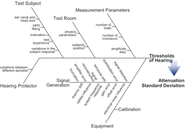
Figure 3 represents the main factors that play an important role in the determination of the HPD attenuation uncertainty.
Thresholds of Hearing Measurement Parameters Calibration Signal Generation Test Subject trun ca tion qua ntiz atio n er
ro r tem pora l d rift am plifie r e
rror sign al re co ns tru ction si gna l d isto rtion elec tric
al n oise influ ence gain err or ther mic drift offs et e
rror syst em fre quen cy resp on se cabl es in
fluen ce Attenuation Standard Deviation Test Room motivation subjects position number of inversions number of trials amplitude step variations in the
subject response HPD fitting
test experience ear canal and
head size physics parameters Hearing Protector variations between different samples Equipment
Figure 3. General list of uncertainties sources.
Considering that the factors presented in Fig. 3 are statistically independent, it is possible using Eq. (1) to determine the measurement threshold uncertainty using the following equation:
(
)
2 22 2 1 2 1 2 n n
threshold u ,u , ,u u u u
u L = + +L+ (17)
where u1, u2, ..., un are the uncertainties of the above mentioned factors.
With the results obtained from Eqs. (5), (14), (16) and (17), it is now possible to estimate the HPD attenuation measurement uncertainty.
NRR
SFUncertainty Calculation
A consequence of the equations presented above is the fact that is possible to use the results obtained through these equations in the calculation of the NRRSF uncertainty as presented below.
The NRRSF value is given by Gerges (1992):
(18) 5 84 − = % SF SNR NRR
Applying again Eq. (1), one writes:
(
84 284 2 ⎥ ⎦ ⎤ ⎢ ⎣ ⎡ ⋅ ∂ ∂ = % % SF
SF u SNR
SNR NNR ) NRR ( u
)
)
(19)The partial derivative above is equal to unity and the uncertainty of the NRRSF measurement can be defined as:
(
%SF) uSNR
NRR (
u = 84
(20)
Therefore, the determination of the NRRSF uncertainty involves
the calculation of SNR84% uncertainty. The definition of SNR84% is (Gerges, 1992): ( ) [ ] [ ( )]
{
( ) [ ] [ ( )] [ ( )] ( )[925 4000 4000 ] 01[904(8000 8000)]
}
1 0 2000 2000 7 92 1 0 1000 1000 5 91 1 0 500 500 3 88 1 0 250 250 9 82 1 0 125 125 4 75 1 0 84 10 10 10 10 10 10 10 10 100 SD a A . . SD a A . . SD a A . . SD a A . . SD a A . . SD a A . . SD a A . . % log SNR ⋅ − − ⋅ ⋅ − − ⋅ ⋅ − − ⋅ ⋅ − − ⋅ ⋅ − − ⋅ ⋅ − − ⋅ ⋅ − − ⋅ + + + + + + + + ⋅ − = dB (21)where Ai and SDiare the attenuation and standard deviation for each
frequency band i.
Using Eq. (21), it can be noted that the value of SNR84% depends
only on the average attenuation and standard deviation for each test frequency band. Its uncertainty can be calculated by:
(
)
(
)
(
)
(
)
(
)
(
8000)
28000 2 8000 8000 2 250 250 2 250 250 2 125 125 2 125 125 2 ⎥ ⎦ ⎤ ⎢ ⎣ ⎡ ⋅ ∂ ∂ + ⎥ ⎦ ⎤ ⎢ ⎣ ⎡ ⋅ ∂ ∂ + + ⎥ ⎦ ⎤ ⎢ ⎣ ⎡ ⋅ ∂ ∂ + ⎥ ⎦ ⎤ ⎢ ⎣ ⎡ ⋅ ∂ ∂ + + ⎥ ⎦ ⎤ ⎢ ⎣ ⎡ ⋅ ∂ ∂ + ⎥ ⎦ ⎤ ⎢ ⎣ ⎡ ⋅ ∂ ∂ = SD u SD SNR A u A SNR ... SD u SD SNR A u A SNR SD u SD SNR A u A SNR ) SNR ( u (22)
The following transformation is now introduced to simplify the equations: ( ) [ ] [ ( )] ( ) [ ] [ ( )] ( ) [ ] [ ( )] ( )
[904 8000 8000 ]
1 0 4000 4000 5 92 1 0 2000 2000 7 92 1 0 1000 1000 5 91 1 0 500 500 3 88 1 0 250 250 9 82 1 0 125 125 4 75 1 0 10 10 10 10 10 10 10 SD a A . . SD a A . . SD a A . . SD a A . . SD a A . . SD a A . . SD a A . . X ⋅ − − ⋅ ⋅ − − ⋅ ⋅ − − ⋅ ⋅ − − ⋅ ⋅ − − ⋅ ⋅ − − ⋅ ⋅ − − ⋅ + + + + + + + = (23)
Using the Eq. (23) and carrying out some mathematical simplification, the partial derivatives of Eq. (22) are written for each frequency band as:
(
[
)]
{
01 75 4 125 125}
125
10
1 . . A aSD
X A
SNR ⎟⋅ ⋅ − − ⋅
⎠ ⎞ ⎜ ⎝ ⎛ = ∂
∂ (24)
( )
[ ]
{
01 75 4 125 125}
125
10 . . A a SD
X a SD
SNR ⎟⋅ ⋅ − − ⋅
⎠ ⎞ ⎜ ⎝ ⎛ − = ∂
∂ (25)
Similar equations for the 1/1 octave frequency band at 250, 500, 1000, 2000, and 4000 Hz numbered (26) to (34).
(
[ )]
{
01904 8000 8000}
8000
10
1 . . A aSD
X A
SNR ⋅ ⋅ − − ⋅
⎟ ⎠ ⎞ ⎜ ⎝ ⎛ = ∂
∂ (26)
( )
[ ]
{
01 90 4 8000 8000}
8000
10 . . A aSD
X a SD
SNR ⋅ ⋅ − − ⋅
⎟ ⎠ ⎞ ⎜ ⎝ ⎛ − = ∂
∂ (27)
To get the uncertainty equation for the standard deviation, the equations above must be inserted into Eq. (22).
Case Study
conversion (equipment), electric and thermal noise from the analog output board used in the measurement system (equipment), subject response variation (test subject). Each of these factors is addressed in the following sections. Other uncertainties were estimated but subsequently disregarded since their contribution to the overall uncertainty was negligible, for the reasons given below. It is important to mention again that these factors change for each HPD test and each measurement system used.
DAQ Board - National Instruments Model: PCI 4451
Computador
Power Amplifier Loudspeakers
Control Software -PEARPA
Hearing Protetor Device
Test Subject
Computer
Figure 4. Measurement system used in the case study.
Amplitude Step
According to ANSI S12.6 (ANSI, 1997), the amplitude step variation shall be defined within the interval from 1.0 dB to 2.5 dB. With the aim of investigating the amplitude step, which corresponds to the least standard deviation (least uncertainties), 312 open hearing thresholds (3 trials with 4 amplitude steps in 26 test subjects) were performed. Some results are presented in Fig. 5, which shows the average standard deviation as a function of frequency bands for the four choices of amplitude step. Duncan’s multiple range tests (Johnson, 1994) were conducted to check if the differences shown in Fig. 5 are statistically significant.
Figure 5. Standard deviation average for the step increment.
The amplitude step of 1.0 dB was considered to give the least standard deviation and consequently the least uncertainty (Lima, 2003). Its uncertainty was estimated as ±0.5 dB with a rectangular distribution. It should be noted that this type of distribution is widely employed in other metrology fields (dimensional applications), when there is no knowledge regarding the type of distribution that best represents the phenomena. This recommendation is considered a conservative approach (INMETRO et al. 1997).
Calibration
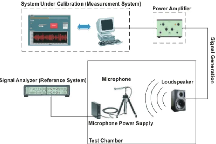
Since the measurement system under study has two different measuring ranges for signal generation, calibrations were performed
in both ranges. Figure 6 shows the system used to calibrate the measurement system employed in HDP tests. It relates the voltage generated by the measurement system to the sound pressure level at the reference point inside the test room. The equipment used for the calibrations was: Brüel & Kjaer Pulse 7700 analyzer, ½” pressure microphone, National Instruments digital acquisition and generation board model PCI 4451, specific module inside PEARPA software for calibration, loudspeakers for noise generation and a power amplifier to drive the loudspeakers.
System Under Calibration (Measurement System)
Power Amplifier
Signal Analyzer (Reference System)
Sig
n
a
l G
e
ne
ra
ti
on
Loudspeaker Microphone
Microphone Power Supply Test Chamber
Figure 6. Calibration setup.
A regression model using the least squares method was developed to represent the calibration curve. The uncertainty contribution from each frequency band due to calibration was calculated from the maximum variation of SPL due to the residual errors of the regression fitting. A rectangular distribution was used and the calibration uncertainty values (rounded to four decimal places) are presented in Tab. 1.
Table 1. Calibration uncertainty values.
Threshold (dB) Frequency (Hz)
125 250 500 1000 2000 3150 4000 6300 8000 Open 0.44 0.54 0.17 0.20 0.30 0.71 0.73 0.23 0.59 Closed 0.43 0.21 0.05 0.39 0.11 0.25 0.45 0.25 0.12
Signal Generation
Since the signal generated is produced mainly by the data acquisition/generation board (PCI-4451 by National Instruments) most of the sources of errors presented below are related to it.
Offset Error
The residual voltage present in amplifiers and converters can produce some errors in the signal generated by the measurement system. Since loudspeakers are not sensitive to DC signals, this source of error was disregarded.
Gain Error
(D/A board used in this study) has a gain error of ± 0.1 dB even after this procedure. For this reason a value of ± 0.1 dB was used to estimate the uncertainty due to the gain error. As the board manufacturer provided no information about the distribution, a rectangular distribution was considered for the calculations.
Signal Truncation
The data to be generated are created from mathematical operations carried out by computer. Since the digital data used in these operations do not have an infinitesimal resolution, these data are often rounded to the next digital value. This rounding produces an error called truncation. In the measurement system, the uncertainty due to truncation was estimated to be ± 0.005 dB with a rectangular distribution.
Quantization Error
Every time a D/A conversion is performed an error is produced since the conversion process is not ideal. This non-ideality is called quantization error and it is dependent on the board resolution and the measuring range used. The board manufacturer suggests the following equation to estimate the quantization error produced by this kind of board:
1
2 −
= NBMR
QE (28)
where QE is the quantization error in volts; MR is the measuring range used in the board (software selectable); NB is the number of bits of the board (resolution).
Applying Eq. (28) to the measuring ranges used in the open and closed threshold determination yields:
mV . MR
QE NB
CT
CT 00305
1 2
2
1
2 − = 16− ≅
= (29)
mV . . MR QE
NB OT
OT 000305
1 2
2 0
1
2 − = 16− ≅
= (30)
where the indices CT and OT represent the Closed Threshold and the Open Threshold, respectively.
The results given above are not adequate because they are expressed in volts, and a propitious result should be expressed in decibels. Since the regression models used are in the exponential form, these values produce different errors according to the sound pressure levels that are generated. If the sound pressure level is low, the quantization error causes a larger uncertainty than when the sound pressure level is higher. To consider this fact, the uncertainty values for the quantization error were calculated from
(
)
Max QE QE
REAL
QE
SPL
SPL
;
SPL
u
=
±
−
+ − (31)where SPLREAL is the sound pressure level produced by a voltage V;
SPL+QE is the sound pressure level produced by a voltage equal to
(V+QE); SPL-QE is the sound pressure level produced by a voltage equal to (V-QE).
To calculate the sound pressure levels mentioned above, the regression models obtained in the calibration processes were used:
B A V ln SPL
⎟ ⎠ ⎞ ⎜ ⎝ ⎛
= (32)
where V is the voltage in volts produced in the board terminals; A
and B are the regression model constants and SPL is the sound pressure level caused by the voltage V at the reference point (a white noise filtered in third octave bands was used). The values of A and B
change for each frequency test.
With the equations presented in (31) and (32) it is possible to estimate the uncertainty for each threshold and each test frequency. A rectangular distribution was adopted.
Noise Error
The board used for signal generation (PCI-4451) is placed in an environment with much interference like video boards, sound boards, hard disks. These components are responsible for electric noise that causes interferences in the original signal. According to the manufacturer, the uncertainties caused by this interference have maximum values that can be estimated by:
SA
LSB
.
E
ElectricNoise=
±
1
0
⋅
⋅
(33)where EElectric Noise is the error due to electrical noise; LSB is the least significant bit; SA is the signal amplitude in volts.
For the same reason explained earlier, an uncertainty expressed in volts can not be used in the global uncertainty calculation. To transform this voltage variation into sound pressure level variation, the following equation was used:
(
)
Max Noise Electric Noise
Electric REAL
Noise
Electric SPL SPL ;SPL
u =± − + −
(34)
The equation presented above is similar to Eq. (31), and the values of SPLREAL, SPL+Electric Noise, and SPL-Electric Noise can also be estimated by Eq. (32). A rectangular distribution was adopted.
Thermal Drift
According to the manufacturer, when the board used for signal generation (PCI-4451) is used in the temperature range from 0ºC to 40ºC, it is not necessary to consider the influence of thermal drifts. As the equipment operates in this range, this source of error was neglected.
Temporal Drift
Small variations in the board behavior during usage can lead to errors. The aging processes become less critical with time since the components present in the board become more stable. For measurements taken within 24 hours of the calibration process, temporal drift can be disregarded. After this period, the manufacturer suggests that an uncertainty of ±15 parts per million should be considered. The following equation was used to estimate the uncertainty due to temporal drift. A rectangular distribution was considered.
(
TemporalDrift TemporalDrift)
Max REALDrift
Temporal SPL SPL ;SPL
u =± − + −
(35)
Frequency Response Function
calibration was performed and the influence of this factor was minimized. As a consequence, this source of error was not considered.
Cables Influence
Cables either function well or not at all. In case of damaged cable, this is easily detected and solved. In the case of functioning cable, this can be modeled as electric components of low resistivity. This resistivity can affect the results (amplitude and frequency variations) if the calibration process is not performed. Since the system was calibrated this source of error was considered indirectly.
Power Amplifier
The power amplifier used to drive the loudspeakers has two major sources of influence: harmonic distortion and electric noise. The influence of the harmonic distortion is too small (less than 0.01% –typical) to be considered. The electric noise was measured to check its levels. The influence of the electric noise is also negligible since it manifests only in the 50~60 Hz (major influence, but also small) and its sub harmonics (minor influence). This factor was, therefore, not considered in the uncertainty calculation.
Signal Distortion
According to the manufacturer, the signal distortion produced by the board is less than the distortion produced by the power amplifier and it was hypothesized that the board has no significant influence in the signal generation process. For the same reasons, this factor was not considered in the uncertainty calculation.
Signal Reconstruction
The analogical signal reconstructed from digital data should ideally have finite amplitude and temporal width equal to zero. Most of the D/A converters maintain a constant voltage in the board terminals until the next sample changes its value, producing an output signal that can be modeled as a series of pulses with variable amplitude.
According to the manufacturer, this non-ideality produces an error that can be modeled by:
A
f f f f sin E
s s
Amplitude ⋅ ⋅
⎟⎟ ⎠ ⎞ ⎜⎜ ⎝ ⎛ ⋅
= π
π
(36)
where A is the signal amplitude; f is the signal frequency; fs is the sample frequency used for generation.
In order to minimize this kind of error, the PCI 4451 has circuits that re-sample the signal with a frequency eight times the original sample frequency. On the other hand, using Eq. (36), it is possible to note that the error is minimized when the sample frequency is higher.
These two pieces of information combined were used to estimate the uncertainty contribution due to the signal reconstruction error at the most critical test band (8000 Hz). The calculation showed that the error is below 0.01%. Since its value is small when compared to the other sources of error, this factor was disregarded.
Variation in the Subject Response
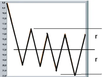
As explained earlier, subjects are needed in order to perform HPD attenuation measurements. The attenuation is a function of the difference between the open and closed hearing thresholds for all the test subjects. The test subject responses are influenced by many factors such as mood, attention, capacity of concentration, ear canal and head size, test experience, ambient pressure and temperature. To estimate this uncertainty it was considered that the hearing thresholds lay between two limits: the maximum peak and the minimum valley of the subject trace. Thus, the mean threshold will be situated at any point between these two limits with the same probability.
The hypothesis above can be modelled by a rectangular distribution with width equal to “r”, where “r” is defined as half of the distance between the highest peak and the lowest valley in the trace, as can be observed in Fig. 7. It is important to mention that the scale in the graph of Fig. 7 is inverted because it follows the same standards used in audiometers.
Other Uncertainties
The measurements were carried out in only one reverberation room qualified according to ANSI S12.6-1997(2000). Therefore, the uncertainty due to reverberation room characteristics was not considered. Since this room is qualified, it is expected that this uncertainty can be neglected.
Figure 7. Level-time domain distribution adopted in the variation in the subject response uncertainty.
Uncertainty Calculation
In order to estimate the uncertainty for the measurement, it is necessary to calculate the uncertainties of each threshold. Since this procedure would be exhaustive if it were presented for each threshold (considering that at least twenty test subjects (plug HPD) are required for each HPD attenuation measurement and each subject produces twenty-eight hearing thresholds (two open and two closed at seven different test frequencies, 7 x 4 = 28), the total number of thresholds would be 560), the uncertainty calculation is demonstrated for just one hearing threshold selected randomly (12th subject at 4000 Hz test frequency, first trial, open threshold).
Table 2. Calculation of the combined uncertainty of the first cycle of the open threshold measurement of the 12th subject at 4000 Hz test frequency.
SOURCE ESTIMATED
VALUE DISTRIBUITION DIVISOR
STANDARD UNCERTAINTY
Amplitude Step uamp 0.50 Rectangular 3 0.288675
Truncation utrunc 0.005 Rectangular 3 0.00288675
Calibration Error ucal 0.7314 Rectangular 3 0.422274
Amplifier gain
error ugain 0.10 Rectangular 3 0.057735
Quantization error uquant 0.4407433 Rectangular 3 0.254463 Electric noise unoise 1.8949E-10 Rectangular 3 1.09402E-10
Temporal drift utemp 9.1688E-10 Rectangular 3 5.29363E-10
Variation in
subject response usubj.resp. 8.25 Rectangular 3 4.76314 utreshold = [(uamp)2
+(utrunc)2 +(ucal)2
+(ugain)2 +(uquant)2
+(unoise)2 +(utemp)2
+(usubj.resp.)2 ]½
4,77976 dB(A)
Table 2 represents the calculation of the combined uncertainty of the first trial of the open threshold measurement, of specific subject (12th), at 4 kHz. From this table, it can be observed that the major influence is due to the variation of the subject response for this particular threshold. Actually, the behaviour presented above repeats for the other thresholds and suggests that the variation of the subject response is really the greatest source of error in the HPD attenuation measurement.
Figure 8 shows the top five average values for the threshold uncertainties for all thresholds, trials, subjects and frequencies. It was calculated by the following way:
1. for each threshold, frequency and subject the uncertainties of each source of error (calibration, subject response, amplitude step) were estimated; 4480 uncertainties were estimated in this step (20 subjects x 4 thresholds x 7 frequencies x 8 sources of error);
2. the average value was taken for each source of error and frequency reducing the 4480 original values to 56 (4480 divided by 20 subjects x 4 thresholds)
3. the average value was taken for each source of error again and the final results are the results presented in Fig. 8 (56 divided by 7 frequencies). The smaller sources of error (truncation, electric noise and temporal drift) were not plotted.
3,7
0,3 0,3 0,2
0,1 0,0
0,5 1,0 1,5 2,0 2,5 3,0 3,5 4,0 4,5
Variation of subject response
Amplitude Step Quantization Calibration Gain error
Sources of Uncertainty
A
ver
ag
e V
al
u
es
fo
r t
h
e
T
h
resh
o
ld
U
n
cer
tai
n
ti
es (
d
B
)
Figure 8. Average threshold uncertainty for the top sources.
After the calculation of the uncertainty values for each threshold, the calculation of the uncertainty for each test subject according to Eq. (16) is performed and the global uncertainty of the attenuation and the standard deviation – Eqs. (5) and (14), respectively – were calculated.
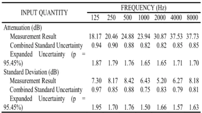
The overall results, rounding the values to two decimals places, are presented in Tab. 3:
Table 3. Hearing protector device measurement result, combined standard uncertainty and expanded uncertainty.
INPUT QUANTITY FREQUENCY (Hz)
125 250 500 1000 2000 4000 8000 Attenuation (dB)
Measurement Result 18.17 20.46 24.88 23.94 30.87 37.53 37.73 Combined Standard Uncertainty 0.94 0.90 0.88 0.82 0.82 0.85 0.85 Expanded Uncertainty (p =
95.45%) 1.87 1.79 1.76 1.65 1.65 1.71 1.70 Standard Deviation (dB)
Measurement Result 7.30 8.17 8.42 6.43 5.20 6.27 8.18 Combined Standard Uncertainty 0.97 0.85 0.88 0.75 0.83 0.79 0.81 Expanded Uncertainty (p =
95.45%) 1.95 1.70 1.76 1.50 1.66 1.57 1.63
Finally, using the values calculated above and applying them in Eqs. (20) and (22) it is possible to obtain the uncertainty of NRRSF
and SNR84%. These results are presented in Tab. 4 (the results are rounded to two decimals places).
Table 4. Application of the hearing protector device measurement result in the determination of the NRRSF and SNR84% uncertainties.
IN P U T Q U A N T IT Y RE S U L T S S N R84% (dB )
M ea surem ent R esult 22.0 6
C om bined S ta nda rd U nc erta int y 0.6 0 E xpa nded U ncerta inty (p = 95,45% ) 1.2 0 N RR S F (dB)
M ea surem ent R esult 17.0 6
C om bined S ta nda rd U nc erta int y 0.6 0 E xpa nded U ncerta inty (p = 95.45% ) 1.2 0
Discussions and Conclusion
The methodology presented in this paper reveals that the calculation of the hearing protector noise attenuation uncertainty is long and arduous because it involves a lot of information. The values presented here are a small portion of the data generated by the formulas shown above.
The uncertainty due to the subject response is the major source of error, accounting for nearly 80% of all sources of error. The sources of uncertainty due to the equipment are small when compared to the subject response. The “amplitude step”, “quantization” and “calibration” appear to have similar contributions to the system studied here. This fact was already expected as mentioned in literature (Brinkmann & Richter, 1986) (Brinkmann, 1988) (Royster et al., 1996).
15 20 25 30 35 40 45
125 250 500 1000 2000 4000 8000
Frequency (Hz)
A
tt
e
nua
ti
on (
dB
)
Measurement Presented New Measurement
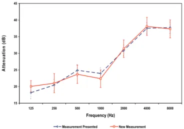
Figure 9. Comparison between two measurements made with the same HPD.
The curves display the measurement results plotted with the uncertainty values presented in Tab. 3. It is clearly shown that the uncertainties and the measurement results are in good agreement at higher frequencies (2 to 8 kHz). In the middle frequency region (500 to 1000 Hz) the measurement results are not in such good agreement, but the uncertainty limits are consistent. Only in the 125 Hz frequency band the uncertainty limits appear to be underestimated suggesting that, for this specific frequency, there must be some source of uncertainty that was disregarded or underestimated.
Another interesting conclusion is that the high number of test subjects in the measurements seems to compensate the wide dispersion in the values for the hearing thresholds, so that the overall uncertainties remain within reasonable values, around 1.5 to 2.0 dB.
This paper is a first attempt in the development of new methodologies for uncertainty estimation for hearing protector attenuation measurements. In this case study some sources of uncertainty were not considered separately. These sources of uncertainty were grouped as can be observed in the variation of subject response. In this case, the effects of fitting, ear canal, head
size, test experience, mood, attention, capacity of concentration, ambient conditions were all considered together.
Acknowledgments
The authors wish to thank CNPq (Conselho Nacional de Desenvolvimento Científico e Tecnológico), of Brazilian Government, for the financial support of this research.
References
ANSI, 1997, “ANSI-S 12.6-1997, American National Standards Method for measuring real-ear attenuation of hearing protectors”. American National Standards Institute, New York, USA, 33 p.
Brinkmann, K. and Richter, U., 1986, “Variability and accuracy of sound attenuation measurements on hearing protectors”, International Congress of Acoustics ICA12, Paper B9-2.
Brinkmann, K., 1988, “Reapeatability and reproducibility of sound attenuation measurements on hearing protectors according to ISO 4869”. PTB internal report.
Gerges, S.N.Y., 1992, “Ruído Fundamentos e Controle”, ISBN 85-900046-01-X, Brazil, 600 p.
Guglielmone, C., 2003, “The uncertainty in the instrumentation for the measurement of noise”, EURONOISE European Conference on Noise Control paper ID: 229-IP/p.1.
INMETRO; ABNT; SDM (Programa RH-metrologia/PADCT-TIB), 1997, “Guia para expressão da Incerteza de Medição”. 1st Brazilian Edition
of the “Guide to the expression of uncertainty in measurement” (ISO; BIPM; IEC; IFCC; IUPAC; IUPAP; OIML), ISBN 92-67-10188-9.
ISO, 1990, “ISO 4869-1: Acoustics – Hearing protectors – Part 1: subjective method for the measurement of sound attenuation”, International Organization for Standardization.
Johnson, R.A., 1994, “Miller and Freund’s Probability and Statistics for Engineers”, ISBN 0-13-721408-1, Prentice Hall, USA, 630 p.
Lima, F.R., 2003, “Development and Metrologic Validation of a Hearing Protector Device Attenuation Measurement System by the Subjective Method”, Doctor Thesis, Federal University of Santa Catarina, Florianopolis, SC, Brazil, 197 p.