P. R. Barbosa
[email protected] Instituto Federal de Educação, Ciência e Tecnologia de São Paulo – IFSP São Paulo, SP, BrazilK. C. O. Crivelaro
[email protected] Univ. Federal de Campina Grande - UFCG Campina Grande, PB, BrazilPaulo Seleghim Jr.
[email protected] Universidade de São Paulo – USP Escola de Engenharia de São Carlos – EESC São Carlos, SP, BrazilOn the Application of Self-Organizing
Neural Networks in Gas-Liquid and
Gas-Solid Flow Regime Identification
One of the main problems associated with the transport and manipulation of multiphase flow is the existence of flow regimes, which have a strong influence on important parameters of operation. An example of this occurs in gas-liquid chemical reactors in which maximum coefficients of reaction can be attained by keeping a dispersed-bubbly flow regime to maximize the total interfacial area. Another example is the pneumatic conveying of solids in which the regimes are associated with safety and energy consumption. Thus, the ability to identify flow regimes automatically is very important, specially to maintain multiphase systems operating according to design conditions. This work assesses the use of a self-organizing map (neural network) adapted to the problem of regime identification in horizontal two-phase flows. In order to achieve extensive results, two different types of two-phase flows were considered: gas-solid and gas-liquid. Tests were made to verify the performance of the neural network model, using data collected at the experimental facilities of the Thermal and Fluid Engineering Laboratory of the University of São Paulo at São Carlos. Results show that the neural network is capable of correctly identifying the regimes. The error percentage is bigger when analyzing the same regime with flow rates different from the one used as training data emphasizing the importance of training signals choice.Keywords: self-organizing map, flow regime, neural network
Introduction
1
The existence of characteristic dynamic patterns or regimes is, certainly, one of the most important subjects in multiphase flows. This justifies the large number of technical and scientific studies in this area, some of which focused on specific technological aspects such as models of pressure drop in specific situations and regimes and others on wider aspects, for example the construction of objective and universal criteria for the identification of multiphase flow regimes. In 1970, researchers in the petroleum industry began to identify certain basic physical mechanisms that could be used to distinguish regimes in liquid columns. Around this time, Taitel and Dukler (1976) published a model, which predicted flow regime transitions based of the physical relations between the following variables: gas and liquid superficial velocity, physical properties of the fluids and pipe geometry. The transition mechanisms are based on physical concepts adapted by experimental observations of two-phase flows (Brill, 1992). Among the many different variables that may be used to diagnose flow regimes, the void fraction is, certainly, one of the most important.
Several methods of measuring this variable have been developed in the last 40 years. A wide range of principles have been applied in order to quantify, or just to reveal the presence of a given phase in the mixture. Some of the measuring techniques require sophisticated equipment such as x-ray absorption spectrometers, while others involve simpler items such as resistance sensors (Moreira, 1989). Examples on tomography techniques for visualization or regime identification can be found at Lehner and Wirth (1999) that obtained the void fraction applying x-ray technique in a downer reactor. Ostrowski et al. (2000) applied capacitance electrical tomography for measurement of dense phase pneumatic conveying, and Xu and Xu (1997) applied ultrasonic tomography in the gas-liquid two-phase flow regime identification.
In gas-liquid two-phase flows it is well-established that an abrupt change in the pressure-drop is frequently associated with a change of flow regime (Wambsganss et al.,1994). Lin and Hanraty (1987) used pressure measurements to detect the intermittent flow
Paper accepted August, 2009. Technical Editor: Celso Kazuyuki Morooka
regime. Osman and Aggour (2002) introduced a neural network model to predict the pressure drop in horizontal multiphase flow. The model was developed and tested on experimental data and a wide range of variables. Sekoguchi et al. (1987) applied a statistical method and the mean void fraction to identify flow patterns. Regarding non-classical techniques of signal analysis, Giona et al. (1994) and Seleghim & Hervieu (1998) used, respectively, fractal techniques and joint time-frequency analysis in the characterization of transitions between horizontal two-phase flow regimes. In this field, the use of neural network techniques to analyze signals from two-phase flows shows great potential (Monji & Matsui, 1998) and many articles have adopted this approach. Crivelaro et al. (2002) used a neural network to process signals emitted by a direct imaging probe in order to diagnose the corresponding flow regime. Smith et al. (2001) utilized self-organizing maps to compare flow regime classifications based on traditional analysis. Statistical values of impedance signals were used as inputs for a neural network, which grouped the results within a number of predetermined categories. Mi et al. (1998) employed a supervised neural network and an unsupervised neural network (self-organizing map) to identify flow patterns, the input signal being a non-intrusive impedance measurement. Cai et al. (1994) demonstrated a technique to classify the patterns of air-water two-phase flow by applying a self-organizing neural network. The principle of the technique lay in the characterization and classification of the turbulent pressure signal in relation to flow regimes. More recent researches have been based on the use of neural networks in association with genetic algorithms and fuzzy logic; a detailed discussion of these techniques may be found in Annunziato and Pizzuti (1999), and Tarca et al.(2002).
transport flow. Chen et al. (1995) studied the distributions of flow regimes and phase holdups in three-phase fluidized beds. Kwak and Li (1996) and Bai et al. (1996) lead wider studies on fluidization regimes. Considering this, the aim of this work is to analyze the application of neural networks in regime identification. Specifically, a self-organizing neural network is implemented and tested in two different experimental circuits: gas-solid and gas-liquid in order to investigate the application of this model in very different regimes cases. In other words, the main objective is to analyze if this tool is capable of being applied at many different multiphase flow situations. This type of neural model (unsupervised) was selected because, in almost every case, data about the regimes are not available. It should be stressed that this question is of great relevance for the efficient operation of equipment and installations involving multiphase fluid transport and represents one of the great challenges nowadays in the petrochemical and thermonuclear industries, among others.
Self-Organizing Neural Networks
An artificial neural network model can be defined as a large number of simple interconnected processing units used to establish an input/output relationship. The self-organizing system considered here belongs to a special class of artificial neural networks (ANN) known as feature maps.
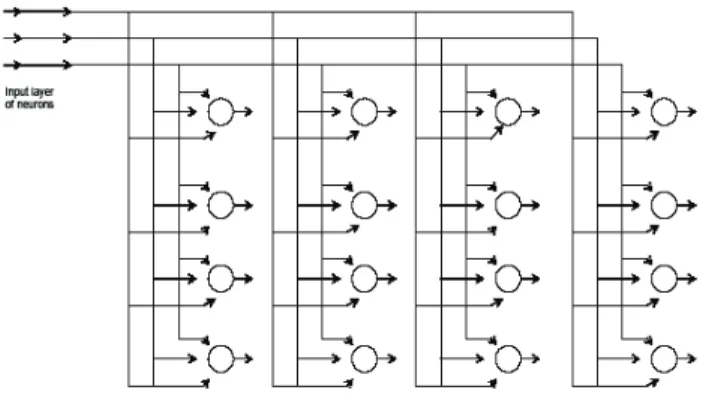
A Self Organizing Map (SOM) consists of neurons organized on a regular low-dimensional grid (usually one or bi-dimensional). Maps of higher dimensions are possible but rarely used. Figure 1 shows a schematic diagram of a bi-dimensional grid, frequently used as a discrete map. Each neuron in the grid is fully connected to the neurons at the input layer.
Figure 1. Bi-dimensional grid of neurons (Haykin, 1996).
From the point of view of the information in the data and how it is visualized, the self-organizing nature of the mapping implies that the statistical and nonlinear metric relations among the n-dimensional input data are converted into simple geometric relations between variables located at the nodes of a bi-dimensional net (Kohonen, 2001). In other words, to the extent that a self-organizing map projects the information contained in the primary data space on to a bi-dimensional network, without altering significantly the topological relations, it may be regarded as a tool capable of creating abstractions. These two attributes – visualization and abstraction of data – are of great importance in complex information-analysis applications, such as the problem of identifying multiphase flow regimes and others involving the use of artificial intelligence (Seleghim Jr., 2002). These networks are characterized by competitive learning, a process in which the output "neurons", or nodes of the map, compete among themselves to become activated while a data-pattern is presented to the inputs.
Eventually, just one output neuron, or one in each local group, becomes the "winner" of the competition and remains active.
The neurons are selectively composed according to the many input patterns or input pattern classes in the context of a competitive learning process. The winner neuron location is arranged according to the other neurons in a significant way inside the coordinate system. It creates a grid for different characteristics of the input patterns.
Let m be the input vector dimension. Let p be any input vector selected from the input space, represented as:
T
[p p1, 2,...,pm]
=
p (1)
The weight vector of which neuron has the same dimension as the input vector. Let the weight vector of the neuron j be denoted by:
T
[wj1,wj2,...,wjm] , j 1, 2,...,l
=
j
W = (2)
where l is the total number of neurons. In order to find the best competition of input and weight vectors, we compare the internal product wTjp for j = 1,2,...,l . Then, the one with the best result is
selected. Furthermore, this neuron fixes the location where the topologic neighborhood of excited neurons is centered.
The best competition criterion, based on the internal product maximization is mathematically equivalent of Euclidean distance (between p and wj) minimization.
The neuron i(p) identifies the closest neuron from input vector
p, and i(p) can be determined applying the condition:
j j
argmin - ,
i(p)= p w j=1,2,...,l (3) This procedure is the essence of the competition process of neurons. The specific neuron i which satisfy this condition is the so called winner neuron for the input vector p.We can verify this in Eq. (3).
A continuous input space of activation patterns is mapped on an output discrete space by a competition process of neurons. Depending on the application, the neural network output can be the winner neuron index (i.e., its grid position) or the weight vector near the input vector or both (Haykin, 1996).
A topographical map is formed in SOM from the input patterns, in which the spatial locations (coordinates) of the neurons in the grid reflect intrinsic statistical features within the input patters – hence the name self-organizing maps (Haykin, 1996). Each input pattern presented to the network is equivalent to a certain region of input space. The position and nature of that region usually vary from one input pattern to the next. All the neurons in the SOM should be exposed to a sufficiently large number of different patterns to ensure that the self-organizing process has the chance of evolving correctly and developing a complete feature map. The layer of nodes in a SOM is arranged initially in physical positions, in conformity with the topology adopted for the map: a hexagonal bi-dimensional grid was used in this work.
Experimental Setup: Gas-Solid
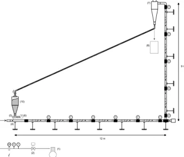
The gas-solid validation tests were done at the experimental facilities of the Thermal and Fluids Engineering Laboratory of the University of São Paulo at São Carlos (NETeF-USP). The pneumatic transport loop, drawn schematically in Figure 2, has a transparent 45 mm inner diameter test section, extending horizontally through 12 m and vertically through 9 m. Air is supplied by a 60 hp screw compressor (1), capable of generating air speeds up to 40 m/s in the transport line. The air flow rate is controlled with the help of a servo-valve (2) and measured by an orifice plate (3), instrumented with temperature and pressure transmitters (differential and absolute). The particulate is introduced in the transport line through a venturi feeder (4), which receives the particulate from a screw conveyor (5). The solids flow rate is controlled by imposing the rotation of the screw conveyor with a frequency converter (6). A cyclone separator (7) is placed at the exit of the test section, from where the particulate may be returned to a separated storage container (8) for batch operation or, alternatively, to a rotary airlock (9) connected to the feeding silo (10) for continuous operation.
Figure 2. Schematic representation of the pneumatic transport test loop at the NETeF-USP.
In this work, the horizontal part of the circuit was focused and the particulate used in the tests was Setaria italica seeds with an average diameter DP = 2.5 mm and an approximately density of
800 kg/m3.
Experimental Setup: Gas-Liquid
In this case the measurements were carried out on the oil pipeline circuit still at the Thermal and Fluid Engineering Laboratory – NETeF-USP which was designed for gas-liquid two-phase flow transient tests. The three-two-phase pilot pipeline sketched in Fig. 3 works with gas-liquid-liquid mixtures and has straight test sections of 12 m length and internal diameter of 45, 30 and 24 mm, placed on a hinged platform that can be inclined up to 100 from the horizontal. A system of tanks installed downstream from the test section is responsible for the primary separation of air from liquid and, subsequently, the separation of oil from water. Centrifugal pumps equipped with 7.5 kW frequency inverters recirculate the liquid phases, controlling the flows with the help of orifice plates installed in the respective injection lines. A 50 kW
screw-compressor supplies the flow of air, which is controlled by servo-valves equipped with flow-sensors. The analytical instruments include rapid-response pressure-sensors to measure total and differential pressure-drops, a capacitance sensor to estimate the phase fraction and an acoustic sensor to produce echograms of the flow. A microcomputer with an analog-to-digital converter is used to acquire the signals from the measuring devices (both operational and analytical), as well as from control devices (servo-valves and frequency inverters). In this study, tests were performed on air-water two-phase flow. The pipeline test section used was a 12 m straight pipe of internal diameter of 30 mm.
DP
P P P P P P P
P P P P
12 m
9 m
(1)
P T
(2) (4) (5) (6)
(7)
(8)
(10)
( (
Figure 3. Sketch of the pilot three-phase pipeline at NETeF-USP.
Neural Models and Results: Gas-Liquid
For each type of horizontal air-water flow pattern, several long duration tests were carried out in the experimental circuit described in section 3. The signals used in the analysis corresponded to measurements of electrical capacitance, pressure-drop in the along pipe and local pressure gradient, collected respectively by a capacitive probe and pressure meters. For each test, the signals were sampled at the rate of 30 Hz until the storage memory was used up (214 samples). Each test lasted for 546 seconds. The classes of test
are defined in Table 1, where Ql represents the liquid (water) mass
flow rate and Qg represents the gas (air) mass flow rate.
Table 1. Classification of regimes tested.
Label Test Ql(kg/s) Qg(kg/s) 1 Smooth
stratified
0.0800 0.0014
2 Wavy stratified 0.0840 0.0075
3 Rough stratified
0.1060 0.0190
4 Intermittent 0.6910 0.0020
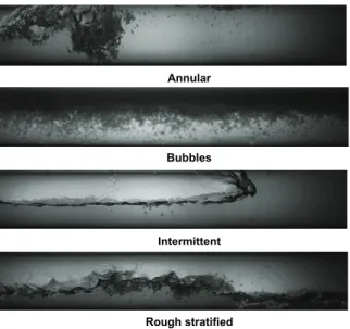
5 Bubbles 7.05 0.0120
6 Annular 0.3500 0.0400
Annular
Bubbles
Intermittent
Rough stratified
Figure 4. Gas-liquid flow regimes.
On the basis of preliminary studies, the architecture of the SOM was defined as a layer of 3 inputs and a grid with 10 neurons. The number of neurons was chosen to enable the network to learn complex tasks by the progressive extraction of significant features from the input patterns (Haykin, 1996). This number is not fixed theoretically and may be chosen equal to the number of classes that the SOM is expected to identify or a larger number. In this case, the network was supposed to identify 6 different flow regimes, but had 10 neurons. In this way, it was possible to discover whether the SOM would autonomously identify 6 regimes and no more, despite possessing a larger number of potential class decoders. After training with the data set, the network did indeed identify 6 different classes of data, which coincided with the flow regimes. The topology of the competitive layer used here was hexagonal, this being preferred for the purpose of unbiased visualization (Kohonen, 2001). The distance calculated between the nodes was Euclidean, which is the commonest distance function found in SOM applications. To train the SOM, data matrices of 300 rows by 3 columns were chosen, small enough for each training run to reach a successful conclusion in a reasonable time, yet not so small that features from the recorded sets of signals would be lost. Ten of these matrices were used for each regime during training. By the end of this training, the SOM had encoded the six distinct flow regimes on six separate neurons (labeled 1, 2, 4, 7, 8, and 10), as shown in Table 2.
Table 2. Neurons identifying the flow regimes in gas-liquid case.
Flow regime Identifying Neuron
Annular 1
Rough stratified 2
Intermittent 4
Smooth stratified 7
Wavy stratified 8
Bubbles 10
To test generalization, characteristic signals for each of the flow regimes were presented to the SOM, in order to verify whether the expected code (neuron index) was output by the ANN.
The signals used in generalization were signals not used previously at training procedure. The data matrices were organized with 16384 rows as discussed before and a part of these matrices were used for training and another part were used for generalization. This kind of test was executed in order to verify if the net was
capable of abstracting the characteristics of different flow regimes, because by this way, it would be able to identify these regimes correctly.
In this context, several simulations of flow-regime tests were performed, using test data not utilized during training and the same result as presented in Table 2 was obtained.
Neural Models and Results: Gas-Solid
The self organizing model used for the gas-solid situation was very similar to the gas-liquid. The topology of the competitive layer used was hexagonal and the distance calculated between the nodes was Euclidean. The input vector has 3900 elements (13 x 300 matrix) and the grid was set to have 6 neurons in order to verify the model ability for the classification of the 4 regimes classified visually. The particulate used in the tests was Setaria italica seeds with an average diameter of 2.5 mm and an approximately density of 800 kg/m3. Several steady state experiments were done with different combinations of gas and solid mass flow rates. The solid mass flow rate (Qsol) ranged from 0.0739 kg/s to 0.1437 kg/s and the
gas flow rate (Qair) from 0.013 kg/s to 0.020 kg/s producing the 4
regimes called in this work: homogeneous, dunes, big dunes, and flow on fixed particle layer (Fig. 5).
Dunes
Big dunes
Homogeneous
Flow on the fixed particle layer
Figure 5. Gas-solid flow regimes.
As the gas-liquid case, several tests were performed. Regarding the training procedure the 4 regimes were perfectly classified in 4 neurons as shown in Table 3.
In this case, two kinds of generalization tests were performed. In the first one, different parts (not utilized) of the signals used for the training procedure were considered (As in gas-liquid case). Note that, although unknown by the net, it implies the use of the same gas and solid mass flow rates as training. The results in this kind of tests were exactly equal to the one showed in Table 3, even changing the way whereby the training data was presented to the ANN.
Table 3. Neurons identifying the flow regimes in gas-solid case.
Flow regime Identifying Neuron
Dunes 5
Big dunes 6
Homogeneous (Homo) 1
Flow on the fixed particle
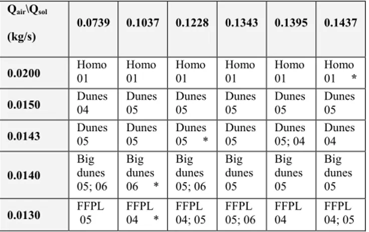
The objective of the second kind of tests was to investigate the net behavior, when evaluating the same regime at different flow rates. The results were summarized on Table 4 where the flow regime name (abbreviation) was compared with the neuron number. The homogeneous and flow on fixed particle layer regimes were abbreviated as Homo and FFPL respectively.
Table 4. Neural net identification for different mass flow rates.
Qair\Qsol
(kg/s)
0.0739 0.1037 0.1228 0.1343 0.1395 0.1437
0.0200 Homo 01 Homo 01 Homo 01 Homo 01 Homo 01 Homo 01 *
0.0150 Dunes 04 Dunes 05 Dunes 05 Dunes 05 Dunes 05 Dunes 05
0.0143 Dunes 05 Dunes 05 Dunes 05 * Dunes 05 Dunes 05; 04 Dunes 04
0.0140
Big dunes 05; 06
Big dunes 06 *
Big dunes 05; 06
Big dunes 05
Big dunes 05
Big dunes 05
0.0130 FFPL 05 FFPL 04 * FFPL 04; 05 FFPL 05; 06 FFPL 04 FFPL 04; 05
The asterisks represent the signals used in the training procedure. For each pair (solid and gas mass flow rate) 10 examples were presented to the net. In the most of cases all of the 10 examples were identified at the same neuron, but there were situations where two neurons were used. The identification for the homogeneous regime was perfect, i.e, even varying the solid mass flow rate the net still indicated the neuron number 1. For the dunes regime approximately 80% of the examples were correctly identified even varying the solid and the gas mass flow rate. For the big dunes and the flow on the fixed particle layer regimes the correct identification percentages were 33% and 50% respectively.
A fact that may explain this lower percentage is that these regimes have mass flow rates very close. It means that probably in the lower part of Table 4 we have lines of regime transitions. It is also important to emphasize that the visual classification was according to the predominant regime, once it is possible to have regime transitions even fixing the mass flow rates.
Conclusions
The employment of a self-organizing artificial network in the identification of two-phase (air-water) flow regimes in a horizontal pipe and gas-solid flow regimes in a pneumatic conveying system has been demonstrated in this study. Data for the air-water flows were collected from a pilot pipeline, designed to allow measurement of capacitance, fluctuating pressure and pressure drop. In the case of gas-solid flow, signals of the pressure drop were collected from 13 sensors and were then used to train the ANN. To verify the ability of the network to generalize, other data obtained from the same experimental circuit were presented to the ANN, i.e. data not used during the training procedure. To validate the proposed methodology, tests of identification were used. Signals characteristic of each flow regime were presented to the ANN, which responded by outputting class codes (index of the activated neurons). The correct identification percentage for the flow regimes achieved by the network was 100%, when using signal with the same flow rates (the same as used in the training phase).
Considering the gas-solid case, tests with different solid and gas flow rates, but still visually representing the same flow regime, were presented to the ANN. The results confirm that the correct identification percentage is bigger for the flow rates near the values
used in the training phase, emphasizing the importance of training signals choice. These results are extremely promising and strongly justify further research in this direction. Firstly, the self-organizing neural network proved to be capable of identifying, completely autonomously, all the main flow-regimes that occurred in the horizontal test-section in the pilot pipeline at NETeF (São Carlos, Brazil). Secondly, the detection-rate with untrained data reached high values in many situations. The study of the optimization of the parameters and hidden variables of the training of the network showed that its performance depended critically on the time of presentation of the training data matrices. Under the right conditions, a self-organizing map is seen to be a very powerful and flexible tool, both for the analysis of experimental data in research and for direct application in the in-line monitoring of industrial processes.
References
Annunziato, M., Pizzuti, S. ,1999, “Fuzzy fusion between fluidodynamic
and neural models for monitoring multiphase flows”, International Journal
of Approximate Reasoning, No. 22, pp. 53-71.
Bai, D., Shibuya, E., Nakagawa, N., Kato, K., 1996, “Characterization
of gas fluidization regimes using pressure fluctuations”, Powder Technology,
Vol. 87, pp. 105-111.
Beale, R.; Jackson, T., 1990, “Neural Computing: An Introduction”, Institute of Physics Publisning, Bristol and Philadelphia.
Bi, H.T., Ellis, N., Abba, I.A., Grace, J.R., 2000, “A state-of-the-art
review of gas-solid turbulent fluidization”, Chemical Engineering Science,
Vol. 55, pp. 4789-4825.
Brill, J.P., 1992, “State of the art in multiphase flow”, Journal of
Petroleum Technology, Vol. 44, No. 5, pp. 538-541.
Cai, S.Q., Toral, H., Qiu, J. and Aecher, J.S., 1994, “Neural network based objective flow regime identification in air-water two-phase flow”,
Canadian Journal of Chemical Engineering, Vol. 72, No. 3, pp. 440-445.
Chen, Z., Zheng, C., Feng, Y., 1995, “Distributions of flow regimes and
phase holdups in three-phase fluidized beds”, Chemical Engineering
Science, Vol. 50, No. 13, pp. 2153-2159.
Crivelaro, K.C.O., Seleghim Jr., P., Hervieu, E., 2002, “Detection of horizontal two-phase flow patterns through a neural network model”,
Journal of the Brazilian Society of Mechanical Sciences, Vol. 24, No. 1.
Giona M., Paglianti, A.E, Soldati, A., 1994, “Diffusional analysis of
intermittent flow transitions”, Fractals, Vol. 2, pp. 256-258.
Hagan, M.T., Demuth, H.B. and Beale, M., 1996, “Neural Network Design”, Boston, PWS Publishing Company.
Haykin, S., 1996, “Neural Network a Comprehensive Foundation”, New York, Macmillan College Publishing Company.
Kwauk, M., Li, J., 1996, “Fluidization regimes”, Powder Technology,
Vol. 87, pp. 193-202.
Kohonen, T. , 2001, “Self-Organizing Maps”, Finland, Springer. Lehner, P., Wirth, K.E., 1999, “Characterization of the flow pattern in a
downer reactor”, Chemical Engineering Science, Vol. 54, pp. 5471-5483.
Letzel, H.M., Schouten, J.C., Krishna, R., van den Bleek, C.M., 1997, “Characterization of regimes and regime transitions in bubble columns by
chaos analysis of pressure signals”, Chemical Engineering Science, Vol. 52,
No. 24, pp. 4447-4459.
Li, J., Kuipers, J.A.M., 2002, “Effect of pressure on gas–solid flow behavior in dense gas-fluidized beds: a discrete particle simulation study”,
Powder Technology, Vol. 127, pp. 173-184.
Lin, P.Y., Hanraty, T.J., 1987, “Detection of slug flow from pressure
measurements”, Int. J. Multiphase Flow, Vol. 13, No. 1, pp. 13-21.
Mi, Y., Ishii, M. and Tsoukalas, L.H., 1998, “Vertical two-phase flow
identification using advanced instrumentation and neural network”, Nuclear
Engineering and Design, No. 184, pp. 409-420.
Monazam, E.R., Shadle, L.J., 2004, “A transient method for
characterizing flow regimes in a circulating fluid bed”, Powder Technology,
Vol. 139, pp. 89-97.
Monji, H., Matsui, G., 1998, “Flow pattern identification of gas-liquid
two-phase flow using a neural network”, 3rd International Conference on
Multiphase Flow, pp. 1-8.
Osman, E.A., Aggour, M.A., 2002, “Artificial neural network model for accurate prediction of pressure drop in horizontal and near-horizontal
multiphase flow”, Petroleum Science and Technology, No. 20, pp. 1-15.
Ostrowski, K.L., Luke, S.P., Bennett, M.A., Williams, R.A., 2000, “Application of capacitance electrical tomography for on-line and off-line analysis of flow pattern in horizontal pipeline of pneumatic conveyer”,
Chemical Engineering Journal, Vol. 77, pp. 43-50.
Sekoguchi, K., inoue, K., 1987, “Void signal analysis and gas-liquido two-phase flow regime determination by a statistical pattern recognition
method”, JMSE International Journal, Vol. 30, No. 266, pp. 1266-1273.
Seleghim Jr., P., 2002, “A New Research Line in Instrumentation and Control of Industrial Multi-Phase Flows” (in Portuguese), “Livre-Docencia” thesis, University of São Paulo, São Carlos, SP, Brazil, 133 p.
Seleghim Junior, P., Hervieu, E., 1998, “Direct imaging of horizontal
gas-liquid flows”, Measurement Science & Technology, Vol. 9, No. 8, pp.
1492-1500.
Smith, T., Ishii, M., Mi, Y., Aldorwish, Y., 2001, “Flow regime identification using impedance meters and self-organizing neural networks
for vertical pipe sizes: 1/2” 2” 4”, 6” ID”, 4th International Conference on
Multiphase Flow, New Orleans.
Taitel, Y., Dukler, A.E., 1976, “A model for predicting flow regime
transitions in horizontal and near horizontal gas-liquido flow”, AIChE
Journal, Vol. 22, No. 1, pp. 47-55, Jan.
Tarca, L.A., Grandjean, B.P.A., Larachi, F., 2002, “Integrated genetic algorithm – artificial neural network strategy for modeling important
multiphase – flow characteristics”, Industrial and Engineering Chemistry
Research, No. 44, pp. 1073-1084.
Xu, L.J., Xu, L.A., 1997, “Gas/liquid two phase flow regimes
identification by ultrasonic tomography”, Flow Measurement and
Instrumentation, Vol. 8, No. 3/4, pp. 145-455.
Wambsganss, M.W., Jendrzejczyk, J.A., France, D.M., 1994, “Determination and characteristics of the transition to two-phase slug flow in
small horizontal channels”, Journal of Fluids Engineering, Vol. 116, pp.
140-146, Mar.
Zijerveld, R.C., Johsson, F., Marzocchella, A., Schouten, J.C., van den Bleek, C.M., 1998, “Fluidization regimes and transitions from fixed bed to