WAGNER JOSÉ GONÇALVES DA SILVA PINTO
NUMERICAL AND EXPERIMENTAL
ANALYSIS OF THE FLOW OVER
A COMMERCIAL VEHICLE - PICKUP
UNIVERSIDADE FEDERAL DE UBERLÂNDIA
FACULDADE
DE
ENGENHARIA MECÂNICA
NUMERICAL
AND
EXPERIMENTAL
ANALYSIS OF THE
FLOW
OVER
A
COMMERCIAL
VEHICLE
-
PICKUP
Undergraduate thesis submitted to the Course of Aeronautical Engineering from the Federal University of Uberlândia as a part of requirement for obtaining the BACHELORS DEGREE ON AERONAUTICAL ENGINEERING.
Tutor: Prof. Dr. Odenir de Almeida
WAGNER JOSÉ GONÇALVES DA SILVA PINTO
NUMERICAL
AND
EXPERIMENTAL
ANALYSIS OF THE
FLOW
OVER
A
COMMERCIAL
VEHICLE
-
PICKUP
Undergraduate thesis APROVED by the Course of Aeronautical Engineering from the Faculty of Mechanical Engineering of the Federal University of Uberlândia.
Thesis Committee Composition:
Prof. Dr Odenir de Almeida
Prof Dr. Francisco José de Souza
Ing. Samara Cunha Rosa (FCA Fiat Chrysler Automobiles)
First of all I'd like to thank the Federal University of Uberlândia (UFU) and more specifically the Faculty of Mechanical Engineering (FEMEC) for providing a high level academic formation that is concluded on the production of this manuscript. I am also grateful to the Fluid Mechanics Laboratory (MFLab) and its staff and colleagues for providing a great ambiance and the means for this work.
I personally thank MSc. Pedro Ricardo for all the support in all aspects regarding the numerical simulations, especially meshing, and Reinaldo Tome Paulino for the amazing work on the test article and all the efforts on improving the wind-tunnel facility. I'm very grateful to Prof. Dr. Odenir de Almeida for the advising and Ing. Samara Cunha for sharing her knowledge and experiences on the matter and promoting an industrial vision on this research.
PINTO, W. J. G. S. P. Numerical and Experimental Analysis of the Flow Over A Commercial Vehicle - Pickup. 2016. 95 f. Trabalho de Conclusão de Curso, Universidade Federal de Uberlândia, Uberlândia.
RESUMO
As pick-ups compreendem uma importante categoria de veículo comercial por combinar o transporte de passageiros e de carga. A presença de uma caçamba aberta é responsável pela formação de uma topologia de escoamento única que é naturalmente de grande interesse para pesquisas dos fabricantes e que vem aos poucos sendo mais discutida em artigos acadêmicos. Este trabalho apresenta um estudo numérico e experimental do escoamento ao redor de uma
pick-up genérica baseada nos líderes de mercado de pick-ups leves do Brasil. O modelo de
pick-up proposto é composto apenas por superfícies planas e cantos vivos e é derivado de um estudo dimensional dos cinco principais modelos da categoria; uma segunda versão é concebida a partir do arredondamento desses cantos. Simulações são realizadas usando as equações de Navier-Stokes médias (RANS) no software STAR-CCM+ com o modelo de turbulência SST k-w; malha é constituída de elementos tetraédricos e o efeito da camada de prisma é estudado. No túnel de vento, anemometria de fio quente e visualização parietal por tufos são utilizados num modelo 1:10 e são usadas como referência para validação inicial dos resultados numéricos. Apesar de uma nova geometria ser testada, resultados são similares aos presentes na literatura. Arredondar o modelo causou uma redução de 30% no arrasto; variações significativas na estrutura global do escoamento na caçamba e na esteira não são observadas. A solução computacional é preparada para o modelo reduzido e para a pick-up em tamanho real em velocidades típicas de rodovia; para a faixa de escalas testadas (Re de 5*105 a 5x10⁶), acredita-se que o problema seja independente do Reynolds, desse modo dados
obtidos em túnel de vento dinamicamente não similares ainda são representativos do escoamento real. Esse trabalho visa servir como referência para análises futuras e deste modo um estudo mais refinado de setup numérico (malha e solver) e a aplicação de outras rotinas experimentais é recomendado. A investigação de mecanismos de redução de arrasto e dos efeitos de outras modificações na geometria é sugerida para as próximas etapas.
ABSTRACT
The pickups correspond to an important category of commercial vehicle once they combine passenger and cargo transport. The presence of an open trunk is responsible for a unique flow topology within a natural great interest for manufacturer's research and that is gradually being more discussed on academic articles. This work presents a numerical and experimental study of the flow around a generic pickup based on the leaders of the light pickup market in Brazil. The proposed pickup model is composed only by flat surfaces and sharp edges and it's derived from a dimensional study of five principal models of the category; a second version is conceived with the application of fillets on those edges. Simulations are performed using Reynolds Averaged Navier Stokes equations (RANS) on STAR-CCM+ solver with SST k-w turbulence model; mesh is constituted of tetrahedral elements and the effect of a prismatic boundary layer is studied. On wind-tunnel, hot-wire anemometry and wall tufts visualization techniques are deployed for 1:10 scale model and serve as a reference for numerical results initial validation. Although a new geometry is tested, the results are similar to previous works. Rounding the model caused a reduction of 30% in the drag coefficient; no significant change is noted on the overall distribution of the structures on trunk and wake. Computational solution is prepared for reduced and full size pickup on typical highway velocities; for the range of tested scales (Re from 5*105 to 5x10⁶), problem is believed to be independent of Reynolds, therefore wind-tunnel data that is not dynamic similar is still representative of real flow. This work is aimed to serve as a benchmark for future analyses so that more refined examination on CFD setup (mesh and solver) and application of other experimental routines are recommended. The investigation of drag reducing devices and the effects of other geometry variations is suggested as next steps.
LIST
OF
FIGURES
Figure 1.1 - Graphic depicting representative horsepower requirements versus vehicle speed for
a heavy vehicle tractor-trailer truck (WOOD and BAUER, 2003)... 7
Figure 1.2 - New passenger cars: CO2 emissions by vehicle segment (The International Council on Clean Transportation, 2011). ... 7
Figure 1.3 - Drag coefficients of different commercial vehicles (HUCHO, 1987)... 8
Figure 1.4 - Example of the effect of an aerodynamic add-on (cab-spoiler) in a truck (HUCHO, 1987). ... 9
Figure 2.1- Flow around a car and major locations of flow separation (HUCHO; SOVRAN, 1993). ... 13
Figure 2.2 - Proposed nomenclature for pick-up parts... 14
Figure 2.3 - Generic pickup model proposed by Al-Garni; Bernal; Khalighi (2003)... 15
Figure 2.4 - Mean pressure coefficient distribution along the symmetry plane on the pickup truck (AL-GARNI; BERNAL 2010)...15
Figure 2.5 - Streamlines of the mean velocity field in the symmetry plane of the wake (left) and on the horizontal plane at z = 15 mm behind tailgate (right) of pickup truck (AL-GARNI; BERNAL 2010)...16
Figure 2.6 - Proposed vortex system of the flow around a pickup (AL-GARNI; BERNAL 2010). 17 Figure 2.7 - Wake shape behind a pickup truck (MOKHTAR; BRITCHER; CAMP, 2009)... 17
Figure 2.8 - Pickup drag coefficient range described on the literature...18
Figure 4.1 - Reference pickup vehicles...25
Figure 4.2 - Test article composing dimensions...27
Figure 4.3 - Pickup models: baseline (left) and rounded (right)... 29 Figure 4.4 - Refinement regions on symmetry plan (L is the pickup length; l is the trunk length;
and W is the pickup width)
Figure 4.5 - Surface mesh of wheel (right) and trunk (left).
Figure 4.7 - Wind tunnel facility...35
Figure 4.8 - Pickup model parts...36
Figure 4.9 - Finalized pickup model...36
Figure 4.10 - Experimental setup...39
Figure 4.11 - Experimental setup (left). On detail (right) the hot-wire support and probe on position P1 and Pitot tube on test section roof... 40
Figure 4.12 - Fluorescent minitufts on car moving at 160 km/h past stationary camera (MERZKIRCH, 1987)...40
Figure 4.13 - Model with wool tufts... 41
Figure 4.14 - Experimental setup for wall tufts test...41
Figure 5.1 - Residuals monitor for simulation with the TETRA (top) and BASELINE (bottom) meshes (in scale, U0 = 25 m/s)...43
Figure 5.2 - Evolution of numerical force coefficients for in scale TETRA (left) and BASELINE (right) meshes, U0 = 25 m/s...43
Figure 5.3 - Evolution of partial average (left) and standard deviation (right) of drag coefficient sequence for baseline and rounded in scale model, U0 = 25 m/s...44
Figure 5.4 - Normalized velocity field on symmetry plane, baseline model for TETRA (top) and BASELINE (bottom) meshes (in scale, U0 = 25 m/s)...45
Figure 5.5 - Streamline on symmetry plane for TETRA (left) and BASELINE (right) mesh (in scale, U0 = 25 m/s)...46
Figure 5.6 - Streamline on center of trunk for TETRA (top) and BASELINE (bottom) meshes (in scale, U0 = 25 m/s)...46
Figure 5.7 - Evolution of Turbulent Kinetic Energy on pickup trunk and wake for TETRA (top) and BASELINE mesh (bottom)...47
Figure 5.8 - Axis system...47
Figure 5.9 - Pressure coefficient on symmetry plane of the cab, bed and underbody for TETRA and BASELINE meshes (in scale, U0 = 25 m/s)... 49
Figure 5.10 - Pressure coefficient on symmetry plane of the cabin rear surface and tailgate for TETRA and BASELINE meshes (in scale, U0 = 25 m/s)... 49
Figure 5.12 - Numerical and experimental velocity profiles at U0 = 16.7 m/s (top) and U0 = 25.0
m/s (bottom). ... 52 Figure 5.13 - Experimental velocity profiles limits for U0 = 16.7 m/s (top) and U0 = 25 m/s
(bottom). ... 53 Figure 5.14 - Spectral energy distribution for velocity signal acquired at P2 (left) and P3 (right), Z = 55 mm (U0 = 25 m/s), using unity as reference for decibels (smoothed curve in red)... 54
Figure 5.15 - Spectral energy distribution of measured velocities on pickup wake at P2 (top line) and P3 (bottom line) for U0 = 16.7 m/s (left column) and U0 = 25.0 m/s (right column), using
unity as reference for decibels...56 Figure 5.16 - Wall tufts on trunk for U0 = 10.0 m/s (left), U0 = 16.7 m/s (center) and U0 = 25.0
m/s (right)...57 Figure 5.17 - Wall tufts on trunk for U0 = 10 m/s (top), U0 = 16.7 m/s (center) and U0 = 25.0 m/s
(bottom)...58 Figure 5.18 - Trunk close wall flow topology for wall tufts test (center) and shear stress
streamlines on trunk surface for TETRA (left) and BASELINE (right) mesh (U0 = 25.0 m/s).
...59 Figure 5.19 - Wall tufts (center) and numerical shear streamlines for TETRA (left) and
BASELINE (right) mesh (U0 = 25 m/s)...59
Figure 5.20 - Normalized velocity field on symmetry plane, baseline model U0 = 25 m/s... 61
Figure 5.21 - Normalized velocity field on symmetry plane, rounded model U0 = 25 m/s... 62
Figure 5.22 - Streamline on center of trunk for baseline (top) and rounded (bottom) models (in scale, U0 = 25 m/s)... 62
Figure 5.23 - Pressure coefficient on symmetry plane of the cab, bed and underbody for baseline and rounded models (in scale, U0 = 25 m/s)...63
Figure 5.24 - Pressure coefficient on symmetry plane of the cabin rear surface and tailgate for baseline and rounded models (in scale, U0 = 25 m/s)...64
Figure 5.25 - Surface pressure coefficient on rear cabin and tailgate exterior (top) and on bed and tailgate interior (bottom) for baseline (left) and rounded (right) models (in scale, U0 = 25
rounded (bottom line) in scale models...69 Figure 5.29 - Pressure coefficient on symmetry plane of the cab, bed and underbody of the
baseline model in all scales...70 Figure 5.30 - Pressure coefficient on symmetry plane of the cabin rear surface and tailgate of
the baseline model in all scales...70 Figure 5.31 - Pressure coefficient on symmetry plane of the cab, bed and underbody of the
rounded model in all scales...71 Figure 5.32 - Pressure coefficient on symmetry plane of the cabin rear surface and tailgate of
the rounded model in all scales...71 Figure 5.33 - Streamline on symmetry plane for rounded model in scale (left) and full size (right)
for U0 = 16 m/s (top), U0 = 25 m/s (center) and U0 = 33 m/s (bottom)...72
Figure 5.34 - Normalized velocity field on symmetry plane at Re1 (top) and Re6 (bottom) for rounded model...73 Figure 5.35 - Streamline on center of trunk for rounded model for two scales: Re1 (top) and Re6
(bottom)...74 Figure 5.36 - Iso-velocity surface for 1/3 of freestream velocity for Re1 (top) and Re6 (bottom)
for rounded model (structures on upstream of the model are omitted)... 74 Figure 5.37 - Drag coefficient for all on scales...75 Figure 5.38- Percentage CD oscillation from all scales average value for baseline and rounded
LIST
OF
TABLES
CHAPTER 1 - Introduction... 6
CHAPTER 2 - Phenomenology... 11
2.1. Fundamentals of Automotive Aerodynamics...11
2.2. Pickup aerodynamics ...14
CHAPTER 3 - Bibliographic review... 19
CHAPTER 4 - Methodology ... 24
4.1. Test Article ...24
4.2. Numerical ...30
4.2.1. Numerical Domain and Mesh ...30
4.2.2. Boundary Conditions and Solver...33
4.3. Experimental setup...35
4.3.1. Wind tunnel Facility and Model ...35
4.3.2. Quantitative method - Hot-wire Anemometry...37
4.3.3. Qualitative method - Wall Tufts ...40
CHAPTER 5 - Results and Discussions ... 42
5.1. Numerical Solution Properties and Validation ...42
5.1.1. Numerical Solution Properties...42
5.1.2. Mesh study ...45
5.1.3. Experimental Results and Validation...50
5.1.3.1. Quantitative - Velocity Profiles ...50
5.1.3.2. Qualitative - Wall Tufts Visualization ...57
5.2. Model study...61
5.3. Scale study...68
CHAPTER 6 - Conclusion ... 77
APPENDIX I ... 82
APPENDIX II ... 83
I - Boundary layer ...84
Introduction
The development of the automotive industry is close related with the technological advances. Significant market and a global concurrence demands constant improvement from the production chain to the final product. In the 20's century, the power plants can be considered the component that most evolved, achieving better performance and less consumption. Following this trend, aerodynamic aspects defined the design of modern vehicles and continue to shape cars.
A compromise between safety, performance and design is performed by each manufacturer. The balance between those domains, directly influenced by financial and productive aspects, is the key to a better vehicle. The variety of models and the complexity of the flow related to each one of them, summed to the dynamics of human occupation and transports needs, demand a continuous evolution of the techniques.
The movement of a car is constraint mainly by two factors: rolling resistance and aerodynamic forces. In general, for commercial vehicles, after 90 km/h, typical highway speed, aerodynamic effects are the major source of those restraining forces, also contributing to instability when lateral forces and moments are taken in account. Therefore, the reduction of drag affects directly the performance and the CO2 emission. Figure 1.1 presents the evolution of
aerodynamic and rolling forces with the speed for a heavy vehicle tractor trailer truck. After 50 mph (80 km/h) the drag is the most important component.
Environmental concerns demand from all transportation industry consistent noise and consumption reduction, so that there are constant reformulation and creation of related legislation, in both national and global context. The new standards play an important role in pushing the development of the industry, as seen in Figure 1.2, the average CO2 emission
7
Figure 1.1 - Graphic depicting representative horsepower requirements versus vehicle speed for a heavy vehicle tractor-trailer truck (WOOD and BAUER, 2003).
Figure 1.2 - New passenger cars: CO2 emissions by vehicle segment (The International Council
A notable example of such initiatives is the INOVAR-AUTO program (Brazilian law number 12,715 of 2012) that intends to promote R&D investments for companies that produce, distribute or present projects to invest in the automotive production in Brazil. One of its pillars is reducing fuel consumption: a decrease of 18.84% by 2017 will result in 2% direct tax deduction for the final product.
Such aspects are aligned with the pursuit for more comfort and economical differentials, pushing the competitors to comprehend and optimize all the phenomenology associated with fuel consumption. The most touched category is commercial vehicles, such as trucks, buses, vans and pick-ups, mostly for its large use and unique geometry that results in bigger drag than for those of passengers' cars (see Figure 1.3). The limitations created by theirs applications requirements, space for cargo, demands more creative solutions and the deployment of multiple engineering tools.
Co
I “1“
Figure 1.3 - Drag coefficients of different commercial vehicles (HUCHO, 1987).
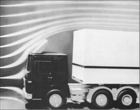
9
geometric modifications, both passive and active flow control techniques can be used to reconfigure flow path, however, the second one must be proven to be energetically lucrative. Spoilers and flaps, for example, are used to drop the strength of recirculation bubbles, to extinguish or retard transition/separation points, reducing and modifying vortex positions, thus decreasing the pressure difference and the related forces. Figure 1.4 exemplifies the effect of a cab-spoiler attaching the flow to the top of the trailer.
Figure 1.4 - Example of the effect of an aerodynamic add-on (cab-spoiler) in a truck (HUCHO, 1987).
Pickups are used as commercial and as passenger vehicles. Despite being similar to SUV's, the existence of the open trunk is unique in terms of airflow behavior and the fact that pickups presents a bigger drag coefficient is more appealing in terms of the pursuit of fuel saving.
(including cars, trucks and buses). In November 2015, pick-ups represented 9% of auto sales in United States according to the Wall Street Journal.
Although the analysis of the external flow around pickups is mostly restrict to the manufactures, it attracts academic work for its complex tridimensional flow, even serving as test case for numerical algorithms. Experimental and numerical works discuss the subject, focused mostly in flow description and drag estimation/reduction techniques.
This study is aimed to the general description of the external flow around a pickup vehicle. A simplified model is prepared from averaged dimensions of the vehicles with the biggest market share in the brazilian light pickups market: Fiat Strada; Volkswagen Saveiro; Chevrolet Montana; Peugeot Hoogar; and Ford Courier. Baseline test article is composed by sharp edges and second version is prepared applying fillets to all external edges.
Analysis is performed numerically using averaged Navier Stokes equations (RANS) and experimentally in a subsonic wind-tunnel (hot-wire anemometry and wall tufts visualization). The experiments are performed with a 1:10 scale version and numerical analyses are done with in scale pickup and full model.
CHAPTER II
Phenomenology
This chapter is dedicated to the description of the fundamentals of automotive aerodynamic analysis and to summarize previous conclusions on the flow present around a pickup.
2.1. Fundamentals of Automotive Aerodynamics
The study of automotive aerodynamics deals with both internal and external flow. Engine feeding, systems cooling, thermal and acoustics comfort are the main focus on the first domain. For the exterior of the car, most important aerodynamic quantities are the forces and momentums, directly influencers of the vehicle stability and consumption.
Lift and drag are the most discussed aerodynamic forces, especially when cross-wind is not considered. The first one is responsible for reducing adherence of the tires and the second one operates against the movement of the automobile. In order to compare forces with virtually any condition (flow velocity and density) and geometries, non-dimensioned coefficients are used, as descripted on the following equations:
n
Drag
'■'!.) =
1
2
pU0A(2.1)
„ Lift
CL
= 1 7 (2.2)2
pU
0A
Those forces are composed by pressure and shear efforts. For bluffy bodies such as a car, the main source of those efforts is the pressure difference created when the air contours such form. An important parameter to describe this phenomenon is the pressure coefficient, CP,
which measures the relation between a static pressure differential and the freestream dynamic pressure:
Cp P-Po (2.3)
where P is local pressure and P0 is pressure on the freestream. For incompressible flow, Cp > 0
indicates that flow is slower than U0 and Cp < 0 means that local flow is faster than freestream
and CP = 1 represents a stagnation point. This parameter is largely used in experimental context
because of simple application (use of pressure tabs on model's surfaces).
The complete description of any fluid dynamics problem has to account for viscous effects. It touches the dynamic of boundary layer detachments and turbulence structures formation. The quantification of those effects is accounted by the Reynolds number, a non-dimensional that compares inertial and viscous effects:
Re
=
(2.4)p
where L is a reference dimension and p is the dynamic viscosity of the flow. In automotive aerodynamics, reference dimension and surface are vehicle's length and frontal area, respectively.
Other important non-dimensional on the analysis of bluff bodies dynamics is the Strouhal number, that correlates vortex shedding frequency and freestream flow velocity:
fC
Co (2.5)
where f is the vortex shedding frequency; and L is the reference dimension (models height for bluff bodies).
13
common around cars (HUCHO, 1987), as illustrated on Figure 2.1. The dynamics of vortexes on rear portion of the vehicle is of great interest and has been largely discussed. The use of simplified geometry, such as the Ahmed body, continues to be an important contribution to the comprehension of those structures and optimization of the automobiles aerodynamics.
Front
End Hood-WindshieldJunction Window JunctionWindshield-Side
Lower Front-Bumper
Region
Left-Front Corner (Top View)
Side Windows (Top View)
Figure 2.1- Flow around a car and major locations of flow separation (HUCHO; SOVRAN, 1993).
2.2. Pickup aerodynamics
Ground vehicles aerodynamics is complex due to the influence of flow from the bottom, top and laterals of the body. The study of pickups has a differential caused by the presence of the open trunk that is impacted simultaneously by all three and its singular components.
The following description and the remaining discussions on this document are going to be presented according to the nomenclature proposed on Figure 2.2. Frontal part of the vehicle is the front end. The underbody is composed by the front overhang (region between front end and frontal wheelbase) and the rear overhang (between rear wheelbase and the end of the pickup). The cab is defined as the upper parts of the vehicle: hood, front-windshield and cabin superior surface. The defined trunk considers the rear surface of the cabin (cabin back surface); the trunk's interior (bed) and laterals walls and the tailgate. Reference dimension are the pickup overall length (L), the bed length (l) and the tailgate height (h).
UNDERBODY L rear overhang ---! front i overhang CAB cabin TRUNK superior surface
Figure 2.2 - Proposed nomenclature for pick-up parts.
15
Figure 2.3 - Generic pickup model proposed by Al-Garni; Bernal; Khalighi (2003).
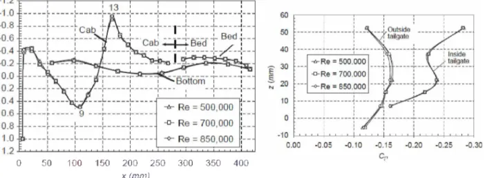
Results of the pressure measured on the model's symmetry plane are presented as the CP evolution graph on Figure 2.4. There is a stagnation region on the front end of the vehicle
followed by a slight acceleration until the frontal tip of hood. Flow decelerates until the joint with the frontal windshield, where it achieves a velocity minimum; next it is reaccelerated until a global CP minimum on cab, gradually pressure coefficient is reduced until cabin back surface.
On bed, all points present a depression. The acceleration of flow caused by the constriction under the vehicles creates a depression on the complete underbody.
0 50 100 150 200 250 300 350 400
x (mm)
Figure 2.4 - Mean pressure coefficient distribution along the symmetry plane on the pickup truck (AL-GARNI; BERNAL 2010).
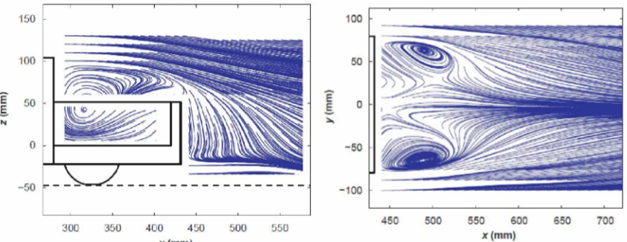
is deviated from the recirculation bubble contacts the outside of the tailgate. On each lateral, counter rotating vortexes are formed by air from laterals and flow leaving the trunk, creating a downwash at the symmetry plane. Vortexes are also created at the end of cabin's roof.
Figure 2.5 - Streamlines of the mean velocity field in the symmetry plane of the wake (left) and on the horizontal plane at z = 15 mm behind tailgate (right) of pickup truck (AL-GARNI; BERNAL 2010).
On back of trunk, pressure is proven to be smaller on the internal surface of the tailgate due to the pressure recovery promoted by the cited downwash. Therefore, a reduction of drag is associated with tailgate up configuration (COOPER, 2004). The results are summarized on the proposed vortex system on Figure 2.6.
Similar effects were obtained by Mokhtar; Britcher; Camp (2009) with a different geometry. A main recirculation bubble on trunk, vortexes on the sides of tailgate exterior and cab, downwash on tailgate are present; CP distribution on symmetry plane is also very similar.
17
Figure 2.6 - Proposed vortex system of the flow around a pickup (AL-GARNI; BERNAL 2010).
Figure 2.7 - Wake shape behind a pickup truck (MOKHTAR; BRITCHER; CAMP, 2009).
In terms of drag force, pickups are known to present higher drag coefficients than SUV's (HOLLOWAY et al. 2009). According to Chen and Khalighi (2015) 70% of the drag is due to pressure difference between front and rear of the pickup. An interest in predicting and reducing this restraining force is noticed on the literature.
Figure 2.8 presents the maximum and minimum CD values encountered on some of the
Besides the existence of such works, the presence of academic publications on this matter remains small. Numerical and experimental standards and methodologies are yet to be defined and specific versions of pickups have to be investigated. This work proposes the description of a light pickup, most common commercial vehicles on Brazilian automotive market. The numerous geometrical variables associated with a pickup have been proven to have complex effects on flow behavior and drag characteristics when varied. The use of simplified model strictly based on light models is aimed to question the geometry influence and to serve as a reference on future works.
0,55
0,45 C 0,40 CD
0,50
---1---1---1---1--- j Illi Illi Illi
______________I_____________r____________▲_____________l_____
r---■
t
:
■
Illi 1 1 1 1
---]---1---T---r---1 1 1 1
1 1 1 1
1 1 1 1
--- ]---1
1
►_________!______________
1 1 1 1 1 1
À 1 1 1 1 1
A
i i i i 1
i i
-- ♦min ▲max
1
■■fit
1 1 x 1 1 ▼
1 1 1
--- 1---1 1 1 --- 1---0,30 0,25 0,35
CHAPTER
III
Bibliographic
review
The study of flow around pickups has been mostly performed in industrial context; therefore there are a small number of open articles on the subject. Even though, a general description can be found and a clear increase of related papers on the last decade is perceived.
The interest in aerodynamically optimize pickups is a longtime concern of the industry. Butz et al. (1987) performed a complete analysis for the development of the 1988 Chevrolet Pickup. A parametric study with ten geometric parameters (such as box length and height and ground clearance) was performed experimentally in a 1/4 scale modular clay model, in a total of 197 configurations. Refrigeration of the engine was considered in wind tunnel testing and acoustic tests were performed with an anechoic model. The effect of the tonneau cover was also discussed for a full tonneau cover and half tonneau, both contributed to the decrease of the drag but the last one was more efficient. Compared to the previous model, the 1987 Chevrolet Pickup, 8% drag and 5dB noise reductions are achieved. A total increase of 0.8 miles per gallon in efficiency was observed, where 75% is a consequence of the aerodynamic improvements.
In a more recent work, Wang et al (2014) used steady CFD analysis. Four design variables (bed length; bed height; cabin height and; ground clearance) were manipulated to achieve the smallest drag coefficient. It was proven that those parameters cannot be isolated in order to reduce drag what confirms the tridimensional aspect of the flow. Only ground clearance showed linear relation and relatively independence to the other variables for the proposed design space. A general conclusion was that a longer bed results in smaller drag. The optimized model has a CD of 0.3163 (9.7% smaller than the original model); the contribution of the tailgate
Furthermore, optimization routines were also performed for aerodynamic add-ons, such as the use of bumps on the rear of the cabin (MOUSSA; FISCHER; YADAV, 2015). The variables were the number and the dimensions of the proposed device equally distributed on cabin roof in the pursuit of a smallest drag. All the analyses were performed with average Reynolds equations (RANS) solver and a reduction of 10% of the drag coefficient was observed. The authors believe that the downward caused by the bumps reduced the strength of the wake thus there was an increase in pressure coefficients in the external face of tailgate.
The use of add-ons to reduce aerodynamic drag is a relatively cheap solution and can be easily design to not affect the functionality of the vehicle. Ha; Jeong; Obayashi (2011) studied the effects of a downward flap on the cab of the cabin. Numerical RANS simulation was performed and wind tunnel testing with a load cell for drag measurement, hot wire anemometer for acquiring the power spectrum density at the tailgate and oil paint on the upper surface of the tailgate for friction lines visualization. The use of the flap resulted in a displacement of the attachment point in the bed, causing more downwash inside the bed, thus reducing the wake strength and consequently the drag force. Another effect was the increase of the pressure coefficient at the cabin back, also contributing to the CD reduction. The best results were
observed for a 12° angle of the flap, with a drag reduction of 5.6% for CFD and 3.6% on experiments.
In 2014, Moussa et al. used the same concept of Ha; Jeong; Obayashi (2011) on a different pickup geometry and performed an optimization of the length and the angle of the flap using global and bounded Nelder-Mead Algorithm. Although using a different model, with completely different bed dimensions, the smallest CD was achieved with the same 12° downward
angle of the flap, and a similar behavior was noted for pressure distribution at the cabin back. Another example is the numerical study of Chen and Khalighi (2015) of three drag reduction devices in a realistic pickup model: boat tail-like extended plates attached to the tailgate; mid-plate attached to the mid-section of the tailgate and; flat plates partially covering the truck bed. All simulations were performed in commercial software FLUENT with a 24 million of elements mesh. The add-ons are formed by non-thickness plates, that is only surfaces with wall conditions. For the 24 tested configurations, the best result (a reduction of 0,021 in CD) was
21
In a mix of add-ons and geometric modifications, Mokhtar et al. (2011) performed a study of two aerodynamic enhancements: a tailgate spoiler and a tapered roof. Numerical simulation is performed for both add-ons and for a generic pickup model using RANS approach. A drag reduction was seen for the two devices; however, the tapered roof was the most effective. A link between the flow behavior and the forces coefficients is observed, the reduction of the recirculation in the wake is related to drag reduction. The speed of the flow changed the degree of contribution of the tested enhancements.
An important aspect of the flow around a pickup is the bed. Many studies are aimed to understand and enhance the phenomenology related to it and find the best configuration in terms of drag reduction. Mokhtar; Britcher; Camp. (2009) tested numerically and experimentally four bed configurations (flat bed, tailgate-off, tailgate down and tailgate-up) in different velocities and yaw angles. The flow behavior was proven to be a function of the walls and boundaries seen in the bed, and the pressure distribution related to those topologies plays a major role in its drag characteristics. The best results were for the flat bed, however for the remaining models (more realistic for the purpose of the vehicle) the tailgate-up is the configuration with the smallest drag.
The same results are seen in the literature relating the smaller pressure in the bed when compared to the values after the force created by this pressure difference is opposite to the flow direction, thus is assumed to decrease the drag.
Conclusion on the influence of speed is also performed. No major differences are seen in flow behavior and a small increase in the drag coefficient is observed. For the yaw angle, the increase is also related to the drag increase. For both parameters, changing the configuration modifies the susceptibility of the force coefficients.
Another contribution of Mokhtar and Camp (2010) was the analysis of the box configuration influence in the drag. For three configurations (open-box, tonneau cover and cap), numerical RANS simulation were performed. For the front of the vehicle (before trunk), there are no variations of the flow. The tonneau cover resulted in a smaller and weaker wake due to the smaller recirculation in bed. For the cap, the wake is larger and even with no separation in cap, a bigger drag is observed.
combinations of bed flow, reverse flow in wake. The smallest drag coefficient is achieved for the short and long bed, geometry in which there is no separation between the recirculation in bed and the tailgate flow. The same behavior is encountered by Al-Garni; Bernal; Khalighi (2003).
A major contribution to the academic study of pickups was made by Al-Garni and Bernal (2003, 2008, 2010). For a proposed generic model, scale 1/12, PIV and pressure measurements (steady and unsteady were performed in wind tunnel for a complete description of flow behavior. The proposed vortex system consists of small counter rotating cab vortex and two bigger structures created at the tailgate. Those two elements create an attachment of the flow in the tailgate, producing a pressure difference between the inner bed and outer bed regions helping to reduce drag, as observed by Cooper (2004). The Reynolds influence on the pressure distribution is considered negligible. Theirs results were used for simulation validation and techniques testing in later works.
Jindal; Khalighi; Iaccarino (2005), performed a RANS analysis of the flow around the model proposed by Al-Garni, using immersive body approach, local grid refinement and adaptive mesh refinement. The domain used for the simulation mimics wind-tunnel boundary condition (no-slip walls) and is formed by 2.1x10⁶ cells. The same behavior for the streamlines and velocities distribution is observed, most significant variation are seen in the underbody and at tailgate vicinity. Limitations of the turbulence method, unsteady effects and the poor refinement of the mesh under the vehicle are pointed as possible sources. The drag coefficient for the simulation showed a 6% deviation from the experimental value.
A study of turbulence models was performed by Holloway; Leylek; York (2009). The calculation setup is based on RANS for 3 different turbulence models: k-e; EVU (unsteady simulation); and SDSM (semi-deterministic stress model). All simulations presented simultaneously very similar results and significant deviations when compared to the wind tunnel values. The authors suggest that the unsteadiness of the problem is not well represented in an averaged approach and even macroscopic parameters such as the drag coefficient are not well predicted.
23
close to the experimental values for the velocity and correlation profiles, the same behavior is achieved for the pressure distribution and flow topology. The friction lines are presented and a recirculation in the base of the windshield was notices. Both turbulence models gave similar results, that way the use of EARSM turbulence model is proven more advantageous for its smaller CPU time. A study scale is suggested.
For a more simplified model, Lee and Parameswaran (2006) performed a transient analysis with the k-£ turbulence model under the Launder-Kato modification. The mesh was produced in ICEM CFD HEXA, no slip condition is assumed for all the walls. No quantitative data is presented, only velocity contours for the symmetry plane and in the truck bed. The flow behavior is reasonable compared to the results presented in literature; however the small amount of data is not representative for more conclusions.
The use of simplified geometry in order to understand the major structures is much disseminated in automotive aerodynamics, being the Ahmed body one expressive example. The same trend can also be seen for pickup inspired geometries. Agelin-Chaab (2014) performed experimental analysis of a 2D bluff-body inspired by pickup trucks geometry. The experiments were made on a water tunnel for different ground clearances and “bed” lengths and heights, PIV and proper orthogonal decomposition (POD) was performed. The description of the flow is similar to the results of Al-Garni (2003) for the 3D generic pickup analysis; however the tri dimensionality of the flow must be taken in account for that analysis. For the tested model, the contribution of the small scale structures (higher order modes) was proven to be the most significant.
Methodology
This chapter is designated for the presentation and definition of the proposed pickup model, and the numerical and experimental setups used on this study.
4.1. Test Article
In order to have a geometry that characterized real vehicles, the used geometry is based upon the most typical models in the light pickups market in Brazil. Table 4.1 presents the number of licensing for this category in July 2014. For the six most licensed models, the Hafei Mini is not considered due to its peculiar geometry; Peugeot Hoggar and Ford Courier are no longer produced, however there are still representative in the fleet.
Table 4.1 - Brazilian Light pickups licensing in July 2014 (FENABRAVE, 2014).
POS. MODEL JULY MARKET JULY JUNE MARKET JUNE
1° Fiat STRADA 12 585 56,28% 10 559 53,78%
2° Volkswagen SAVEIRO 7 294 32,62% 6 721 34,23%
3° Chevrolet MONTANA 2 446 10,94% 2 319 11,81%
4° PEUGEOT HOGGAR 23 0,10% 23 0,12%
5° HAFEI MINI 11 0,05% 13 0,07%
6° Ford COURIER 1 0,00% - 0,00%
TOTAL 22 360 100,00% 19 635 100,00%
25
the Ford Courier). It's observed that the geometrical variations between versions of the same vehicle are small and possible mistakes regarding the considered variety are negligible.
Fiat Strada
Volkswagen Saveiro
Chevrolet Montana
Peugeot Hoggar
Ford Courier
Figure 4.1 - Reference pickup vehicles.
Total of 26 external dimensions are obtained from manufactures website, customer manuals and from photographs analyzing using the software ImageJ. For the image processing, one known dimension (total length or total width) is used to set the scale of the photo in pixels/mm and the scale is confirmed for another known dimension (total height). A total of 10 images encountered on manufacturer's websites and publications on specialized media were used: two for the Fiat Strada; two for the Volkswagen Saveiro; one for the Chevrolet Montana; three for the Peugeot Hoggar; and two for the Ford Courier. A mean error of 4.5% is observed for all the scale tests. The acquired dimensions are presented on Figure 4.2 and Table 4.2.
overall length of the bed of the Ford Courier was not considered due to its discrepancy of the values presented for other models.
MODEL
Table 4.2 - Pickup models dimensions
LABEL DESCRIPTION STRADAFiat SAVEIROVW MONTANAChevrolet HOGGARPeugeot COURIERFord
A track front [mm] 1,425 1,429 1,550.124
B track-rear [mm] 1,390 1,490.71 1,439 1,396.631
C windshield front height [mm] 1,094.033 995.319 1,078.657
D1 overall height [mm] 1,402.433 1,550 1,578 1,524 1,477
D2 overall height (with cab rack) [mm] 1,525 1,497 1,630 1,577.886
E ground clearance [mm] 170 231.381 264.286 203.052 265.281
F hood front height [mm] 839.401 861.571 877.176 821.207
G1 overall width [mm] 1,664 1,708 1,700 1,668 1,793
G2 overall width (with mirrors) [mm] 1,906 1,893 1,918 2,020.399
H cabin lateral angle [deg] 62.152 66.371 57.995 62.808
I hood angle [deg] 11.725 9.951 10.305 12.799 9.039
J1 approach angle [deg] 25.849 32.59 24.109 20.925 25.769
J2 departure angle [deg] 26.743 27.77 25.322 21.915 25.755
K windshield angle [deg] 31.858 30.669 30.196 29.403 31.855
L rear of cabin angle [deg] 23.039 12.45 23.374 27.512 9.866
M front overhang [mm] 790 744.893 844 792.59 679.998
N wheelbase [mm] 2,718 2,750 2,669 2,745 2,893.417
O rear overhang [mm] 901 872.091 1,001 883.325 884.271
P overall lenght [mm] 4,409 4,493 4,514 4,526 4,457
Q1 box height [mm] 1,249.249 1,228.855 1,195.558 1,143.976 1,058.722
Q2 box interior height [mm] 525 464
R box lenght [mm] 1,685 1,615.461 1,737.357 1,706.814 1,760.316
S width between wheelhouses [mm] 1,090 920 1,119 1,100
T1 box interior width [mm] 1,230 1,340 1,240
T2 box width [mm] 1,350
V overral lenght at box [mm] 1,640 1,680 1,816+
LEGEND
1,000 1,000 1,000
data from manufacturer and specialized publications data from images analysing
27
R
Figure 4.2 - Test article composing dimensions.
To achieve an understanding of the general flow around a pickup, the model is simplified: no air inlets or outlets are modeled; underbody is simplified; there are no rear viewers, wheels housing or any attachments in the model, thus dimensions labelled as ‘D2', ‘G2' and ‘S' are not considered on this study. The simplified design (sharp edges and plan surfaces) does not reproduces any of the original vehicles; however the use of a more generic body is aimed to clarified macroscopic effects seen in outside flow of a pickup, especially in bed, and ignores the design choices of the manufactures.
For each dimension, a simple mean operation is applied in order to achieve a geometry that represents in general the pickups on the road; values are presented on Table 4.3. The maximum and minimum values of the dimensions and the standard deviation and coefficient of variation are also presented. As seen in Ha; Obayashi; Kohama (2009), the bed geometry plays a key factor in the produced aerodynamic structures and consequently in the drag of the vehicle, the use of five references could represent a more global geometry with could be seen as more
illustrative.
observed for the angular values and are due to the difficult of the image analyzing, especially for the rear of cabin angle (L). The geometry of the wheels is based on the standard tire of four of the reference pickups: the 175/70 R14 (18 cm wide and external diameter of 60 cm).
Table 4.3 - Statistics of dimensions analysis.
LABEL MAXIMUN MINIMUN MEAN STANDARDDEVIATION VARIATIONCOEF. OF
A 1,550.12 1,425.00 1,468.04 71.11 4.8%
B 1,490.71 1,390.00 1,429.09 46.46 3.3%
C 1,094.03 995.32 1,056.00 53.11 5.0%
D1 1,578.00 1,402.43 1,506.29 68.94 4.6%
D2 1,630.00 1,497.00 1,557.47 58.85 3.8%
E 265.28 170.00 226.80 40.92 18.0%
F 877.18 821.21 849.84 24.59 2.9%
G1 1,793.00 1,664.00 1,706.60 52.00 3.0%
G2 2,020.40 1,893.00 1,934.35 58.27 3,0%
H 66.37 58.00 62.33 3.43 5.5%
I 12.80 9.04 10.76 1.49 13.9%
J1 32.59 20.93 25.85 4.26 16.5%
J2 27.77 21.92 25.50 2.22 8,7%
K 31.86 29.40 30.80 1.07 3.5%
L 27.51 9.87 19.25 7.65 39.7%
M 844.00 680.00 770.30 61.47 8.0%
N 2,893.42 2,669.00 2,755.08 83.74 3.0%
O 1,001.00 872.09 908.34 52.82 5.8%
P 4,526.00 4,409.00 4,479.80 47.46 1.1%
Q1 1,249.25 1,058.72 1,175.27 76.35 6.5%
Q2 525.00 464.00 494.50 43.13 8.7%
R 1,760.32 1,615.46 1,700.99 55.78 3.3%
S 1,119.00 920.00 1,057.25 92.29 8.7%
T1 1,340.00 1,230.00 1,270.00 60.83 4.8%
T2 1,350.00 1,350.00 1,350.00 -
-V 1,680.00 1,640.00 1,660.00 28.28 1.7%
29
The overall dimensions are of the same magnitude of previous works, as presented in Table 4.4, however specific dimensions (such as bed height and length) and the proportions of the models are not the same and comparisons between results must be made with care in regard of those differences. In order to achieve a convenient blockage factor on experimental testing, 5 % according to Hucho (1987), 1/10 scale is adopted. The model presents 205.58 cm2 of frontal area that equals a blockage ratio of 5.71 % on wind tunnel.
Table 4.4 - Overall dimensions and blockage ratio of generic pickup models in the literature.
MODEL Al-Garni
(2003) (2009)Ha Mokhtar*(2010) (2006)Lee lenght [mm] 447.98 432 407.4-528.6 5,300 432
height [mm] 150.63 148.8 167 1,900 123
width [mm] 170.66 152 183.5 1,780 152
frontal area [m2] 0.0206 0.019 - 2.545
-blockage ratio 5.71 % 6% - 0.78 %
-*numerical simulation
The model is designed in the software CATIA V5R20 using the dimensions presented on Table 4.3 and the cited tire diameter. The model is made entirely composed by sharp edges and flat surfaces; the three views plan is presented on Appendix I. Later on this work it is referenced as “baseline”. In order to comprehend the effects of the sharp edges, a second version of the model (“rounded” version) is prepared by adding a fillet of 15 mm on all the external edges and a fillet of 6 mm on the exterior of the bed; the bed interior is the same for the baseline model. Both models are illustrated on Figure 4.3.
4.2. Numerical
4.2.1. Numerical Domain and Mesh
The mesh is prepared in software ANSYS ICEM CFD 16.0, meshing software that allows the use of CAD exported geometry from multiple software; capable of structured and unstructured meshing; and to export them for a number of solvers such as ANSYS FLUENT; Star-CCM+, CFD++ and OpenFOAM. The relative high controllability of shell and volumetric elements parameters allows the creation of sophisticated domain discretization.
The complete domain surfaces (model and boundaries) are prepared on CATIA using both generic pickups presented on section 4.1. The files must be converted to an older file format of CATIA (.MODEL, from CATIA V4) in order to be imported on ICEM CFD.
The numerical domain dimensions are based on the car length L and follow the proportions used by Ha; Jeong; Obayashi (2011). As summarized on Figure 4.4, the inlet is placed forward the model at a distance of 10L, the outlet is located 20L downstream the model, the superior limit of the domain is at 10L (instead of 30L) of the ground and the lateral limit is placed after 7.5L the model. Only half of the model is simulated with 0.06 % blockage ratio.
Figure 4.4 - Refinement regions on symmetry plan (L is the pickup length; l is the trunk length; and W is the pickup width)
31
- trunk density: element size of 2 mm, corresponds to the trunk and the closer portion of the wake. It starts at the end of the rear surface of the cabin; therefore it is bigger for the rounded geometry. Labelled as (A) on diagram;
- wake density: element size of 5 mm, comprehends both the later wake and the underbody of the model; (B) on diagram;
- inner density: size of 10 mm, englobes all the pickup and affects both before and after the model; (C) on diagram;
- outer density: size of 40 mm, an expansion of the previous density; (D) on diagram.
- wheel density: variable size, minimum of 0,5 mm on the contact with the ground; one for each wheel, not represented in the diagram.
On the rest of the domain - represented as (E) - the element size is defined as the length of the pickup (447 mm).
Wheels and trunk surface mesh is defined using the blocking feature of the software for triangular elements and are illustrated on Figure 4.5. The pre-mesh is later converted for unstructured mesh.
Figure 4.5 - Surface mesh of wheel (right) and trunk (left).
layer is 0.05 mm height - y+ ~ 3.5 for Schlichting skin-friction formula, U0 = 25 m/s) on the ground and on the vehicle (labelled BASELINE); mesh is redone for a better numerical convergence (in order to reduce shrunken and distorted pyramidal elements), however all the domain definitions presented on Figure 4.4 are maintained to grant a reasonable comparison between results. The same study was intended to be performed for the rounded geometry, but numerical convergence was not reached for the mesh with no prismatic boundary and all preliminary results are not presented. Thus, the ROUNDED mesh contains also tetra and prismatic elements (same size and distribution cited previously).
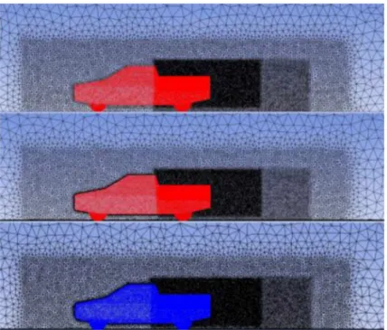
The main refinement regions and the boundary elements are depicted on Figure 4.6, with represents the surface mesh on the symmetry plane and the pickup model for the three meshes.
Figure 4.6 - Numerical surface mesh on symmetry plane and pickup (from top to bottom: TETRA, BASELINE and ROUNDED).
33
focus of describing the mean flow structures, meshes are considered reasonable, especially for the available computational capacity.
The tested flow velocities (16.67 m/s; 25 m/s and 33.33 m/s) are constrained to wind tunnel performance and correspond (in terms of Reynolds number) to a very slow pickup speed (6 to 12 km/h). For the chosen scale, dynamic correlation is achieved for a ten times bigger velocity (166.7 to 333.3 m/s) within would consist in an important Mach value and level of compressibility.
To question the validity of the use of in scale model for the description of the flow around the real size pickup, both the baseline and the rounded model are tested at the same freestream velocity with an enlarged geometry: a simple scale transform is performed for the mesh, extending the size of the elements for a factor of 10 in all three directions, maintaining for each individual case (TETRA, BASELINE and ROUNDED) the same elements geometry and distribution.
4.2.2. Boundary Conditions and Solver
All the numerical analyses are performed using the steady Reynolds Averaged Navier Stokes equation (RANS) in commercial software STAR-CCM+, distributed by CD Adapco Inc.
The turbulence model is SST k-w, proposed by Menter in 1994, with the standard coefficients. It presents good behavior in adverse pressure gradients and separating flow conditions (HA; JEONG; OBAYASHI, 2011). Solution is based on the segregated flow model (2nd order upwind convection scheme), with all y+ wall treatment. Fluid is incompressible air (standard properties: 1.18415 kg/m3 density and 1.85508x10’5 Pa.s dynamic viscosity);
reference pressure is also let on standard (P = 101,325 kPa).
For the proposed discussions, a total of 18 simulations are performed, considering: three freestream velocities; three meshes (corresponding to the two geometries) and two scales (full size and in scale), as summarized on Table 4.5.
Table 4.5 - Simulations Matrix.
MODEL baseline rounded
MESH TETRA BASELINE ROUNDED
SIZE Full Scale Full Scale Full Scale
«r
.E
oD
16.667 x x x x x x
25.000 x x x x x x
33.333 x x x x x x
The CFD calculations are done in a workstation with an Intel Core i7-3930K (3.20 GHz) processor with twelve cores (six physical) and 48.0 GB RAM memory. For the presented meshes, mean iteration time is of 12 seconds when all cores are used.
35
4.3. Experimental setup
This section presents all experimental assets and techniques used on this work.
4.3.1. Wind tunnel Facility and Model
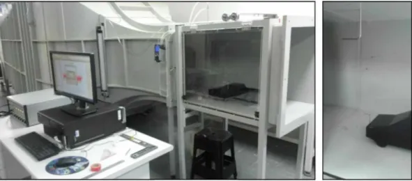
The facility is an open wind tunnel with a test section of 60 x 60 cm of the External Aerodynamics Research Center (CPAERO) of the Federal University of Uberlândia, presented on Figure 4.7. Flow momentum is created by a rotor of 12 blades driven by a 25 HP electrical engine on the upstream of the wind tunnel. Air velocity is driven by an electrical inverter (output from 0 to 60 Hz).
It is instrumented with pressure tabs and an analogic manometer. A Pitot tube and a digital manometer can also be used for calibration.
Figure 4.7 - Wind tunnel facility.
In order to perform the experiments presented on this work, improvements were made on the wind tunnel. The concerning results and general wind tunnel flow description procedures are
The baseline model is printed using a MakerBot 3D printer, model Replicator 2x, with an ABS filament of 1.5 mm diameter. The geometry is prepared under the same CATIA model that generated the meshes for CFD analysis, thus the chamfer in wheels is also present. The generation of STL files (for the printer) follows the standard exportation parameters and the tessellation is prepared on printer manufacturer's software (MakerBot Desktop). Due to limitations regarding the printer size, the model is printed in four parts, as presented in Figure 4.8. Printer resolution is 0.5 mm and the level of infill density is 10%.
Figure 4.8 - Pickup model parts.
Superficial texture and distortions observed on the largest pieces required later preparation for assembling the parts and smoothing the external surfaces and the contacts. The finalized model, presented on Figure 4.9, is painted black to achieve better contrast on the qualitative flow visualization tests.
Figure 4.9 - Finalized pickup model.
37
4.3.2. Quantitative method - Hot-wire Anemometry
This technique uses the magnitude of heat that is transferred from a thin wire to a passing flow in order to measure it speed. Electric current is applied to the wire, generating electrical power (P) proportional to the current magnitude (I) and the wire resistance (Rw):
P = I2Rw. Once temperature of the wire is steady, it means that the amount of energy given to
the wire equals what is being dissipated to the flow, thus, convective energy is measured. With access to the voltage difference that created the current, we are able to the monitor the amount energy.
Dissipated energy via convection can be related to the flow velocity using a power law correlation for the Nusselt non-dimensional number. The following equation was proposed by King on 1914, known as King's law:
I2
R^=E2
=(T
w- T
o)(A + BUn)
(4.1)where E is the voltage; Tw is wire temperature; T0 is a reference temperature; U is the velocity of
the flow and A, B and n are coefficients obtained on calibration. With measured voltages, those coefficients can be obtained using equipment such as a Pitot tube or another hot-wire anemometer system placed at the same flow or a calibration nozzle.
Measured voltages are commonly related to flow velocity using two different equations presented next:
■ Power law (based on King's law):
(4.2)
■ 4th degree polynomial equation:
U
=
Co + CiEc
+ C2E2
+C
3E
2 +C
3E2 (4.3)where A, B, n, and C0 to C5 are the calibration constants and Ec is a corrected voltage.
Celsius degree change) and fluid compressibility. When low speeds are considered, natural convection also influences. More details on the technique itself can be seen on DANTEC documentation (J0RGENSEN, 2004), where this short description is based.
Important features of the flow can be analyzed using the signals obtained with hot wire anemometry. Besides mean velocity, U0, two interesting parameters when describing turbulence
can be derived: the standard deviation of the velocity, URMS, and the turbulence intensity, Iturb (its
adimensionalized version). All formulations are presented on following equation:
N
Uo
i = 1
Uf; hurb
U
rms (4.4)where Ui is a acquired velocity; and N is the total number of acquired values.
Global distribution of turbulent scales and vortex shedding frequency can be defined with spectra of the recorded signal using Fourier Transform for a discrete signal:
N
DSP(k) = x(j~)
exp( — 2m/AQ
(y-1)(A'-1)
i=i(4.5)
Values can be presented in the decibels scale using a reference value (Eref):
(DSP\
DPS
dB
= 20logio\—
-)
(4.6) \Eref /The hot-wire anemometry is used to produce velocity profiles upstream and downstream the model. All measurements are performed using DANTEC Dynamics StreamLine Pro Anemometer System. A 1D hot-wire probe (55P11) is attached to a 90° support and connected to one of the constant temperature anemometer (CTA) modules of the StreamLine Pro frame. The acquisition module is connected to a National Instruments A/D converter which sends data to the computer via a USB port. The system control and data exporting is done with the manufacturer's software, StreamWare Pro. Figure 4.10 illustrates the experimental setup.
39
before the model (P1); 50 mm and 92.57 mm - approximately tailgate height h and its first multiple - after the model (P2 and P3, respectively).
Measurements of the stream wise velocity with a 1D hot-wire probe are performed for a distance of the ground from 5 mm to 170 mm, each 5 mm (total of 34 measurements points per position).
The sampling frequency is 2 kHz (acquisition period of At = 0,5 ms) for a total of
N
= 32,768 sample points (acquisition time of T = 16.383 seconds). A Pitot tube is placed on the roof of the test section and a digital manometer displays the free stream velocity. This indication is used to define global freestream flow stagnation and start anemometer acquisition.Calibration is performed using the StreamLine Pro Automatic Calibrator for 20 velocities between 1 to 27 m/s, logarithmic spaced. Indicated pressure and temperature are P = 91.85 kPa and Tabs = 27.30 °C. The 4th degree polynomial function is chosen as the calibration law and
temperature correction is not applied. All unmentioned parameters are set default on the acquisition software and the post processing is performed on software MATLAB.
Figure 4.11 - Experimental setup (left). On detail (right) the hot-wire support and probe on position P1 and Pitot tube on test section roof.
4.3.3. Qualitative method - Wall Tufts
In order to describe flow direction and detached/recirculation zones close to model's surface, wall tufts technique is applied. Important features of close surface flow can be easily pointed with this technique: when flow is laminar, tufts are aligned with flow direction and describe a relatively steady dynamics; on turbulent/unsteady regions, the movement of tufts is highly oscillating; zones where tufts are elevated are the ones within separated/adverse flow (MERZKIRCH, 1987). Disturbances caused by the presence of the tuffs and theirs attachments assets (tape or glue) must be accounted. This method is largely applied in both aeronautical and automotive domains (example presented on Figure 4.12).
41
For this study, 15 mm long wool tufts are attached on pickup walls. Tufts are not placed on the front end; on the underbody, only the wheels and the final part of the trunk (rear overhang) are discretized. An average distance of 5 mm is considered between the lines of tufts. Figure 4.13 presents the model with the tufts.
Figure 4.13 - Model with wool tufts.
The tests are recorded with a high definition camera posed on a tripod, as seen on Figure 4.14. The effects on the trunk are also registered from the top via a hole on test section roof using a cell phone camera. Recording are made on three flow velocities: 10.0, 16.7 and 25.0 m/s. On this document, representative frames of those videos are presented.
Results
and
DiscussionsThis section is dedicated to the presentation and discussion of both experimental and numerical results.
5.1. Numerical Solution Properties and Validation
First chapter is dedicated to present the simulation characteristics and the influence of boundary layer discretization for the baseline model, numerical results and the validation of CFD solution. The flow around both geometries is discussed next. Final part contains the results of the performed scale study.
5.1.1. Numerical Solution Properties
This section is dedicated to present the aspects of numerical solution and to describe the proposed convergence criteria. If not settled contrary, the results presented on this section are for the in scale model, freestream at U0 = 25 m/s and meshes with and without prismatic
boundary.
43
Figure 5.1 - Residuals monitor for simulation with the TETRA (top) and BASELINE (bottom) meshes (in scale, U0 = 25 m/s).
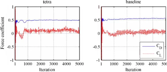
In order to define a number of minimum iterations to obtain a representative solution, velocity field on symmetry plane and force coefficients are monitored. Figure 5.2 presents the evolution of CD and CL for the two meshes.
tetra
Iteration
Figure 5.2 - Evolution of numerical force coefficients for in scale TETRA (left) and BASELINE (right) meshes, U0 = 25 m/s.
baseline 1 ---■
--1 ---■---■---.--- •---1 1000 2000 3000 4000 5000
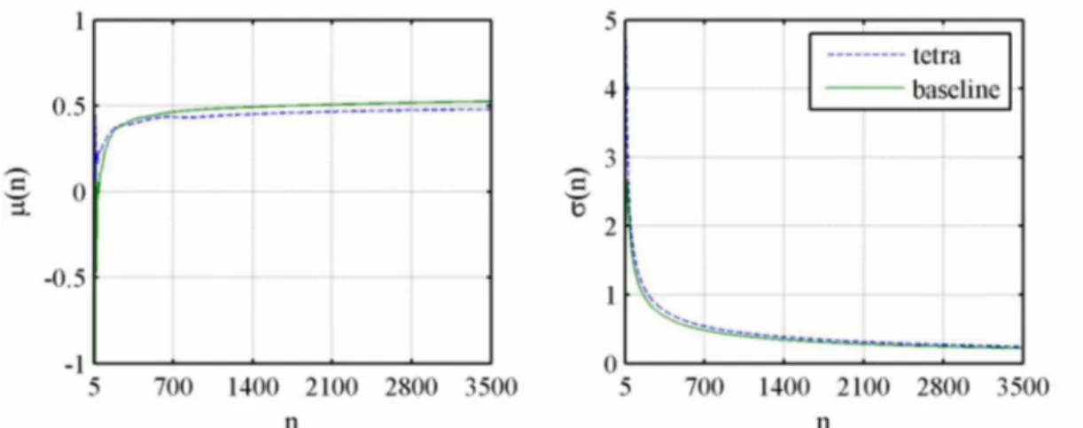
Stopping criteria is defined based on drag coefficient convergence. A sequence
l = {CD,i ; i = 1,2,3,...}, where i represents a iteration, is statistically convergent if and only if its
sequence of partial averages, p(n), converges and its sequence of partial standard deviations, o(n), converges to 0 (BURGIN; DUMAN, 2006). Figure 5.3 shows the evolution of the mean and standard deviation of the numerically obtained CD sequences, starting at iteration 5. For both
geometries, convergence is defined visually within 3,000 iterations.
Figure 5.3 - Evolution of partial average (left) and standard deviation (right) of drag coefficient sequence for baseline and rounded in scale model, U0 = 25 m/s.
Similar behavior is observed in all calculations and the simulations are stopped with 3,500 iterations; the additional 500 are used for force coefficients prediction. Standard deviation of the considered CD values (from iteration 3000 to 3500) is on the order of 0.005. At the last
iteration mass imbalance for the complete domain is around 1x10⁻⁴ %.
For the proposed number of iterations, convergence is not well defined for the lift coefficient with the TETRA mesh. According to Guilmineau (2010), poor discretization of the underbody may lead to poor CL prediction, but this aspect alone does not invalidate the solution.
For BASELINE mesh, 40 elements are added between the ground and the model (the two prismatic boundaries) and convergence is similar to the observed for drag coefficient.
45
5.1.2. Mesh study
For the baseline model, simulations are performed for two different meshes: TETRA with no prismatic layers; and BASELINE with 4 mm boundary layer discretization. The influence of the proposed refinement is discussed next. Simulations for in scale, 25 m/s flow are used for the comparison.
Figure 5.4 presents the normalized velocity field for both meshes. The coarse mesh (TETRA) has globally a similar velocity field, with a big recirculation bubble on the trunk and above the hood. However, the poor modeling of the flow contact with the surfaces (minimum element size of 2 mm) of the geometry caused a simpler reproduction of the smaller structures and their effects. For the BASELINE mesh, the ground detachment and the shear layer on pickups underbody is more well-defined. Also, a recirculation region on front overhang and a boundary layer growth on cabin top are present and a higher wake is existent.
Figure 5.4 - Normalized velocity field on symmetry plane, baseline model for TETRA (top) and BASELINE (bottom) meshes (in scale, U0 = 25 m/s).
the recirculation center downstream, as showed on Figure 5.5. The detachment on trunk is placed at 24% of bed's length for the refined mesh and at 2% of l for the TETRA mesh. The smaller vortexes formed on lower exterior part of tailgate are numerically instable and vary in position and shape for a relatively low number of iterations and cannot be accountable for comparing the meshes.
Figure 5.5 - Streamline on symmetry plane for TETRA (left) and BASELINE (right) mesh (in scale, U0 = 25 m/s).
Inside the trunk, a different behavior is present. Figure 5.6 has the streamlines for both meshes on the center of the trunk horizontal plane. The central recirculation is much smaller due to the presence of a more important vortex on the cabin back surface, at the center of the trunk. On wake, there are no significant changes on the streamlines distribution.
47
Solution for the BASELINE mesh contained a more energetic wake (Figure 5.7). The vortex on cab is more developed for the chosen scale and a slower dissipation is achieved; turbulent energy is also more prominent close to the ground.
Figure 5.7 - Evolution of Turbulent Kinetic Energy on pickup trunk and wake for TETRA (top) and BASELINE mesh (bottom).
The discretization of the boundary layer caused variations of the pressure evolution on symmetry plane of the model. The differences are going to be commented on the following paragraphs and a discussion on the structures themselves is presented on the section 5.2. Results are presented following the axis system on Figure 5.8 and are adimensionalized using the model overall length (L), bed length (l) and tailgate height (h).