Lat. Am. j. solids struct. vol.11 número2

(1)

Abs tract

The paper presents an analysis of the possibility of increasing the accuracy and stability of machining of low-rigidity shafts while ensuring high efficiency and economy of their machining. An effec-tive way of improving the accuracy of machining of shafts is in-creasing their rigidity as a result of oriented change of the elastic-deformable state through the application of a tensile force which, combined with the machining force, forms longitudinal-lateral strains. The paper also presents mathematical models describing the changes of the elastic-deformable state resulting from the application of the tensile force. It presents the results of experi-mental studies on the deformation of elastic low-rigidity shafts, performed on a special test stand developed on the basis of a lathe. An estimation was made of the effectiveness of the method of control of the elastic-deformable state with the use, as the regu-lating effects, the tensile force and eccentricity. It was demon-strated that controlling the two parameters: tensile force and eccentricity, one can improve the accuracy of machining, and thus achieve a theoretically assumed level of accuracy.

Key words

low rigidity shaft, control of machining accuracy, mathematical models of machining, efficiency, mechanics of machine tools

Method of control of machining accuracy of low-rigidity

elastic-deformable shafts

1 INTRODUCTION

A half or all machine parts are rotating elements: shafts (ca. 40%), discs, sleeves, cylinders etc. Among those, up to 12% are low-rigidity shafts (Pus et al., 1982).

A highly important, and at the same time complex problem is the achievement of the assumed ac-curacy of machining and operational reliability of low-rigidity shafts. Such shafts are elements of many assemblies of various machines and devices, and find applications in, among others, aerospace industry, precision mechanics, tool-making industry (special tools), automotive industry. They are characterised by disproportion in overall dimensions and low rigidity in specific sections and direc-tions. Stringent requirements are also applied in terms of the geometric shape, mutual positioning of surfaces, linear dimensions and quality of surface finish.

A n to ni Ś_wić1_{, Dari us z W o}ł_os1_,

G rze go rz L itak*,2

1 _{Institut of Technological Information} Sys-tems, Lublin University of Technology, Nadbystrzycka 36, PL-20-618 Lublin, Poland

2 _{Department of Applied Mechanics, Lublin} University of Technology,

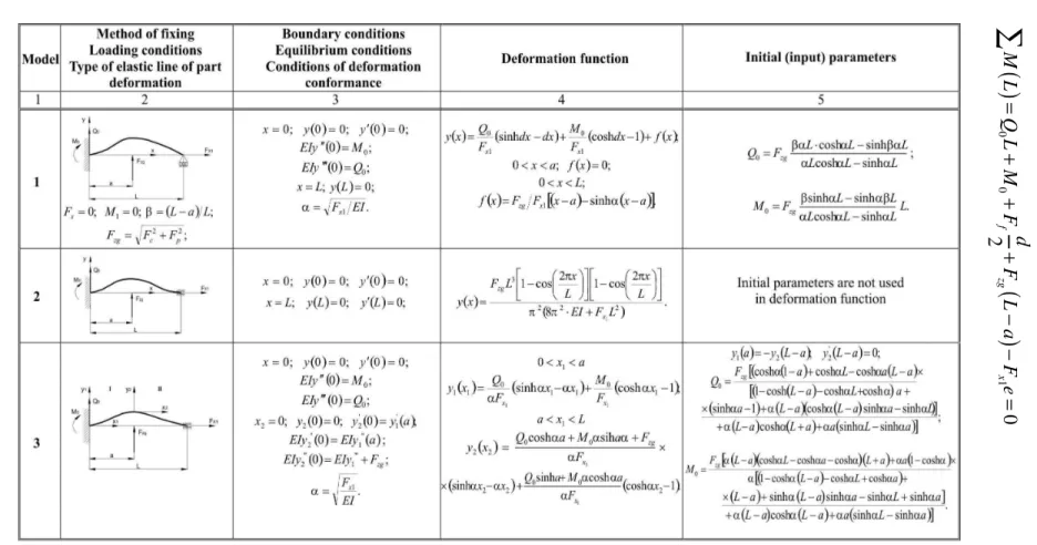
Nadbystrzycka 36, PL-20-618 Lublin, Poland

Received 06 Feb 2013 In revised form 03 May 2013

(2)

G. Litak et al. / Method of control of machining accuracy of low-rigidity elastic-deformable shafts 261

Latin American Journal of Solids and Structures 11(2014) 260 - 278

The specific nature of machining of similar parts causes that the primary difficulty relates to the achievement of the required parameters of the accuracy of form, dimensions and surface quality. Low inherent rigidity and relatively low rigidity of the shaft, compared to the stiff assemblies of the machine tool, cause the appearance of vibrations under specific conditions. The process of machin-ing interferes with and destabilises many factors (large free distortions of shafts, vibrations in the tool-object system, breaking of chips etc.), which causes a reduction in the accuracy of machining (Cardi et al., 2008; Hassuiand and Diniz, 2003; Jianliang and Rongdi 2006; Litak et al., 2004; Li-tak and Rusinek 2012; Qiang, 2000; Altintas, 2000).

The traditional methods of achieving accurate machining of low-rigidity shafts, based on multi-pass machining, lowered parameters of machining, steadies and additional treatments and manual lap-ping, cause a significant lowering of efficiency, and in many cases preclude the achievement of re-quired reliability; also, they are incompatible with the contemporary requirements of automation, they are uneconomical and inefficient.

The initial studies on the dynamic response of a rotation shaft subjected to a moving load has been done by Katz et al. (1988). Especially, they focused on the dynamical effects accounted by different approaches: Euler-Bernoulli, Rayleigh, and Timoshenko beam models for a simply supported rotat-ing shaft leadrotat-ing to the changes in rotor response. This problem was generalized to a three-directional load moving in the axial direction by Ouyang and Wang (2012).

In the context of a regenerative cutting process, chatter vibrations response of the workpiece mod-elled as a flexible beam were also studied by Altintas (2000), Tusty (2000), Chen and Tsao (2006), and more recently by Bisu et al. (2009a; 2009b), Cahuc et al. (2010), Han et al. (2012).

2 MATHEMATICAL MODELS OF MACHINING OF ELASTIC-DEFORMABLE SHAFTS

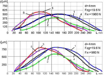
One of the effective ways of improving the accuracy of machining of parts of this type is increasing their rigidity as a result of oriented change of their elastic-deformable state, through the application of a tensile force which, combined with the machining force, forms longitudinal-lateral strains. As shown by experimental studies, increase of rigidity of parts with diameters from 2 to 6 mm and length from 100 to 300 mm, with their loading with a tensile force within the range from 980 to 1960 N, leads to a reduction of elastic strain by from 80 to 20%, respectively. Furthermore at di-ameters d = 8 – 12 mm such a loading reduce elastic stain by 5 –7%. Increasing of d > 16 mm at a given length has practically no effect on the value of static stiffness and, correspondingly, on the deformation of the parts (Jianliang and Rongdi, 2006; Ś_wić_{et al. 2010).}

Analysis of the effect of the tensile force on the static rigidity of machined elements can be per-formed with the use of the model in Table 1, line 1. The model does not provide an adequate de-scription of the behaviour of the elastic line at various methods of fixing. This means that, in the model in question, the element fixed in the tailstock of the lathe has both the possibility of linear displacement along the axis of the part and the possibility of free rotation of the section at the point of fixing. In many cases, such a method of fixing does not lead to a reduction of deformation in the machining zone.

(3)

To minimise elastic deformation, it is also possible to control the angle of rotation of the part section at the point of fixing, through the application of a tensile force shifted with relation of the axis of the centres (Ś_wić_{et al. 2010). This kind of fixing can also be represented as a moving rotary}

support (Tab. 1, line 4).

The fundamental feature of the presented schematic is the application of the control moment at the point of fixing of the machined part – through eccentric tension. The application of a single controllable force factor – eccentric tension – permits the generation of two force factors at any predefined section of the part, and in the machining zone in particular: the longitudinal force Fx1

and the bending moment M2 = Fx1 · e, counteracting the machining forces, i.e. the oriented

elastic-deformable state of the shaft.

The application of tensile forces with a shift relative to the axis of the centres at both ends of the machines shaft – in this case the fixing can be represented as a moving rotary support (Tab. 1, line 5) – permits the control of the position of the part axis from two sides at any position of the cutting tool, relative to the length of machining. Moreover, it is possible to use a special fixture for mobile tensioning in the machining of long shafts with low rigidity (Tab. 1, line 6).

The specifics of elastic-deformable loading of low-rigidity parts, with eccentric compression in machining operations, are taken into account in model 7 (Tab. 1).

In Table 1 the following symbols are used:

Fx1 tensile force;

Fzg bending force;

Fc, Fp, Ff are two bending force and axial components;

e eccentricity of tensile force in tension;

M1 moment generated by the axial component Ff of the machining force;

x1, x2, x3 current coordinates at each of the sections;

a distance between the cutting edge (point of load application) and the point

of fixing of the part in the spindle;

b,c other characteristic distances along the shaft;

d diameter of the machined part;

L length of the shaft;

Q0 and M0 initial parameters: perpendicular force and moment at the point of the fixing

of the part, respectively.

One of the methods that permit the generation of a mathematical model describing the kind of elastic line, with relation to the part parameters and to the parameters of the process of machining (loading forces) is the energy method of Ritz, by means of which the deformation functions were obtained for a tensioned rod with an end fixed rigidly (Tab. 1, line 2).

(4)

y

_iIV

−

α

2

_y

i "

=

0

₍₁₎

where:

α

₌

F

x1

EI

, E – modulus of elasticity, I – moment of inertia of the section.

In the simplest case, the only disturbance of the elastic line is located at the point of machining, i.e.

i

₌

_∈

{

_{1, 2}

}

₍₂₎

The solution of equation (1) can be written in the simplified single mode form (for symmetric situation - model 2 instead of hyperbolic functions the trigonometric ones are used) (Young et al., 2003):

y

_i

( )

x

_i

=

A

_i

sinh

α

_x

i

+

B

i

cosh

α

x

i

+

C

i

x

i

+

D

i (3)

and in the case of (2):

y

1

( )

x

1

=

A

1

sinh

α

x

1

+

B

1

cosh

α

x

1

+

C

1

x

1

+

D

1

y

2

( )

x

2

=

A

2

sinh

α

x

2

+

B

2

cosh

α

x

2

+

C

2

x

2

+

D

2

.

⎧

⎨

⎪

⎩⎪

(4)

Taking into account that

M

₁

( )

x

₁

=

EI

_⋅

y

₁";

F

₁

( )

x

₁

=

EI

_⋅

y

₁''';

M

₂

( )

x

₂

=

EI

_⋅

y

₂";

F

₂

( )

x

₂

=

EI

_⋅

y

₂''', from the boundary conditions (column 3, Tab. 1) in each system of coordinates at

x

1

=

0

, deformation

y

1

( )

0 =

0

, angle of rotation of section

y

1 '

0 ( )

=

0

_and

_EI

_⋅

_y1

''

( )

0 ₌

_M

₀_,

EI

_⋅

y

1 '''

0 ( )

=

Q

0, the constant coefficients were determined as follows:

A1=

Q0

EIα2 ,

B

1

=

M

0

EI

α

2 ,

C

1

=

−

Q

0

EI

α

2 ,

D

1

=

−

M

0

EI

α

2 , (5)

and the equation of deformations on section I, taking into account (5) and the terms for the deter-mination of α_{can be written as:}

y

1

( )

x

1

=

Q

0

α

_F

x1

sinh

α

_x

1

−

α

x

1

(

)

+

M

0

F

_x1

cosh

α

_x

1

−

1 (

)

(6)

Coefficients A2, B2, C2, D2 were expressed from the boundary conditions x2 = 0, conditions of

bal-ance and compensation of deformations

y

1

'

a

( )

=

y

2

'

0 ( )

,

EIy

1 ''

a

( )

=

EIy

2 ''

0 ( )

,

EIy

1 ''

a

( )

+

F

_zg

=

EIy

2

'''

0

(5)

A

₂

=

Q

0

cosh

α

_a

₊

_M

0

α

sinh

α

a

+

F

zg

α

3

_EI

,

B

₂

=

Q

0

sinh

α

a

+

M

0

α

sinh

α

a

α

3

_EI

,

C

₂

=

Q

0

cosh

α

_a

₊

_M

0

α

sinh

α

a

+

F

zg

α

3

_EI

,

D

₂

=

Q

0

sinh

α

a

+

M

0

α

sinh

α

a

α

3

_EI

,

(7)

And the equation of deformation on section II can be written as:

y

2

( )

x

2

=

Q

0

ch

α

a

+

M

0

α

sh

α

a

+

F

zg

α

_F

x1

sinh

α

_x

2

−

α

x

2

(

)

+

Q

0

sinh

α

a

+

M

0

α

cosh

α

a

α

_F

x1

cosh

α

_x

2

−

1 (

)

.

₍₈₎

Equations of deformations on sections I and II, for the case of model 4 (Tab. 1) and the other cases of loading considered, obtained in an analogous manner, are presented in column 4, Tab. 1.

The values of the initial parameters Q0 and M0 were determined at extreme conditions at the

end of the rod:

y

2

'

L

₋

a

(

)

=

0

₍₉₎

and the equations of deformations at the end of the deformed rod:

y

₁

( )

a

=

₋

y

₂

(

L

₋

a

)

(10)

The results of solving equations (9) and (10) are given in column 5, Tab. 1.

At eccentric tension (model 4, Ff ≠ 0, e ≠ 0) the differential equations (1) on each of sections I

and II have the form:

y

1

IV

₋

_α

1 2

y

1 ''

=

0

₍₁₁₎

y

2

IV

_−α

2 2

y

2 ''

=

0

₍₁₂₎

where:

α

1

=

F

_x1

−

F

f

EI

,

α

2

=

F

_x 1

EI

,

and the solution of (11) and (12) is written as (3), taking into account α₁_{on section I. Substituting the boundary conditions, conditions of balance and conditions} of simultaneity of deformations (column 3, Tab. 1) into equations (11) and (12), a description of deformations was obtained, as presented in column 4, Tab. 1.

The initial parameters Q0 and M0 were determined through conditions (9) and the equation of

(6)

G. L itak e t al . / Me th od o f c on tr ol of m ac h in in g a cc u ra cy o f l ow -ri g id ity e la sti c-de for m abl e sha ft s 26 5 La tin A m er ic an Jour na l of S ol ids a nd S tr uc tur es 11 (20 14 ) 26 0 - 2 78

M

L

(

)

∑

=

Q

0

L

+

M

0

+

F

f

d

2 +

F

zg

L

−

a

(

)

₋

F

x 1

_e

=

0

(13 )

Table 1 Conditions of loading of parts with control of the elastic-deformable state (see various conditions of loading of parts with control of the elas-tic-deformable state (1 – Model; 2 – Method of fixing, loading conditions, type of elastic line of part deformation; 3 – Boundary conditions, equilibrium

(7)

Ta

b

le

1

(co

n

ti

n

u

ed

(8)

Ta

b

le

1

(co

n

ti

n

u

ed

(9)

and the obtained values of Q0 and M0 are given in column 5, Tab. 1.

A specific feature of the problem of control of elastic deformations of an elastic-deformable part under consideration, with two-sided eccentric tension (Tab. 1, line 5), is the ease of determination of the initial parameters Q0 at known M1 = Fx1e1 and M2 = Fx2e2 from the conditions of the

bal-ance of forces, relative to the axes of coordinates (

∑

_Y

=

0

_{) and of the balance of moments}

(

M

b

∑

=

0

_{– columns 3 and 5). At the same time, it becomes more complicated to determine the}

angle of rotation Q0, at which the term sought was obtained from equations (10) and presented in

column 5.

For a long part loaded with a tensile force, the calculation schematic was presented in the form of a beam twice statically indeterminate (Tab. 1, line 6), loaded with bending force Fzg, moment

M

₁

₌

F

_f

_⋅

d

2

and longitudinal forces Ff and Fx1. The values of the forces and moments are definite,

with

F

_x

1

>

F

f and

F

f

>

0

, therefore to the left from point A the beam is always in a state of

ten-sion, and the value of Ff can be negative as the direction of the working travel f changes. In the

case of diameter equal to d1 on the left section of the part (from point D to 0) and diameter d2 (to

the right from D), the axial moments of inertia of the cross-section will equal, respectively,:

I

₁

₌

π

d

1 4

64

,

I

2

=

π

d

₂4

64

, and parameters

α

2

=

F

_x 1

EI

2

,

α

1

=

F

_x₁

+

F

_f

EI

₁ . When support A moves to

the right, point D moves with it at the same velocity, and distance b has a constant value. Dimen-sion a changes within the range of 0 ≤ _a≤ (l – _a). To solve the double statically indeterminate

prob-lem of longitudinal-lateral bending of the beam, under loading with the moving tensile force Fx1, the

left and the rights parts of the beam were analysed.

From the boundary conditions and the conditions of mutual interaction of deformations (Tab. 1, line 6) the functions of deformations (column 4) and the initial parameters (column 5) were ob-tained.

(10)

Figure 1 Estimatedrelations of elastic deformation changes of a shaft (numbers from 1 to 5 correspond to the numbers designating

the models in Table 1).

3 EXPERIMENTAL STUDIES

The experimental studies of elastic deformations of low-rigidity shafts were conducted on a special test stand, constructed on the basis of a lathe (Fig. 2).

A shaft (1) is aligned in the lathe grip between a standard compression dynamometer (2) type DOSM–3–02 (measurement range from 19.6 to 196.0 N), mounted by means of a bracket (3) in the cutter holder (4) of the lathe. The radial component of the cutting force Fp was estimated using the

dynamometer (2). Registration of elastic deformations was conducted by means of an electromag-netic displacement transducer (9) with a recorder unit (10). The transducer (9) was mounted in a holder (8) on a plate (6) positioned on the guide rails (5 and 7).

(11)

The experimental stand was used to test the elastic deformations of shafts with diameters

d = 2 –18 mm and lengths of 100, 200 and 300 mm. The maximum deformation of the part, under

tension with the axial force Fx1, decreases in a non-linear manner in accordance with the equations

given above (Tab. 1).

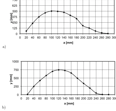
Experimental results (model 1) are shown in Fig. 3. The shaft was loaded with axial force Fx1 =

1960N (a) and 980N (b), respectively, while the lateral force was Fzg = 19.6 N. The measurements

accuracies were 0.4 N and 0.01mm for Fx1 axial forces and displacements, respectively.

Based on the further experiments performed (to model 2) one can state that the discrepancy be-tween the analytical results and the experimental data is from 3 to 12%. The calculations were made with the use of model 4, with the assumption that

F

x1

≠

0

, e=0 fully correspond to the data

obtained from model 1.

Certain discrepancies between the results could also result from the assumptions adopted in the selection of calculation scheme.

a)

b)

Figure 3 Experimental dependence of elastic shaft deformation (of length L = 300 mm and diameter d = 4 mm ) loaded with axial force

Fx1 = 1960N (a) and 980N (b). The lateral force Fzg = 19.6 N, fitted according to the model shown in Table 1, case 3.

On the basis of the calculations of elastic deformations caused by axial tension, and also on the basis of experimental data, it can be stated that at any point on the part (L/d = 15 – 50 within the range of shaft diameters under consideration), and at the point of machining in particular, situated

0 125 250 375 500 625 750

0 20 40 60 80 100 120 140 160 180 200 220 240 260 280 300

y [

m

]

a [mm]

0 250 500 750 1000

0 20 40 60 80 100 120 140 160 180 200 220 240 260 280 300

y [

m

]

(12)

directly beneath the cutting edge (x = a), the value of elastic deformation of the shafts tested can be significantly reduced through the selection of a suitable tensile force Fx1 and eccentricity e (Halas

et al., 2008; Ś_wić_{et al. 2011).}

In the development of technological methods for the control of grinding accuracy of low-rigidity shafts the elastic-deformable state can be generated by means of longitudinal compressive forces, shifted relative to the axis of the centres or applied additionally to the ends of the parts by means of bending moments.

4 OPTIMISATION OF PARAMETERS OF AN ELASTIC-DEFORMABLE STATE

The calculation scheme of the forces acting on the shaft and the elastic line of the shaft are present-ed in Table 1 (line 7). The application of compressive forces, shiftpresent-ed relative to the axis of the cen-tres, was considered as method of generation of a bending moment applied to the face of a low-rigidity shaft and as a technological premise for the control of machining accuracy.

In the case of a beam compressed with a longitudinal force and transmitting any lateral force, the solution of equation (1) can be presented in the form:

y

=

y

₀

+

y

₀'

α

_x

₊

_y

0 ''

1 −

_cos

α

_x

(

)

+

y

₀'''

(

α

_x

−

_sin

α

_x

)

₊

_{f x}

( )

,

(14)

where:

y

0,

y

0 '

,

y

0 ''

,

y

0 '''

– deformation, angle of rotation, second and third derivatives at the origin of the system of coordinates, respectively,; f(x) – function of the effect of lateral loads.

The equations of the lines of elastic deformations on sections I and II have the form of:

y

_I

=

y

₀'

α

x

+

y

₀''

(

1 −

cos

α

x

)

+

y

₀'''

(

α

x

−

sin

α

x

)

,

y

II

=

y

0 '

_α

x

+

y

0 ''

1 −

cos

α

x

(

)

+

y

0

'''

_α

x

−

sin

α

x

(

)

+

f x

( )

.

⎧

⎨

⎪

⎩⎪

(15)

The initial parameters, in accordance with the conditions adopted earlier (Tab. 1) are as follows:

(

)

[

]

(

)

(

)

+ ⎭ ⎬ ⎫ ⎩ ⎨ ⎧ ₋ ₋ − − + − − = L L L L L L L L F F y x zg

_βα

α

βα

β

α

cos sin 1 cos

cos sin cos 1 1 ' 0

(

)(

)

, sin sin cos cos 1 1 cos sin 1 2 ⎥ ⎦ ⎤ ⎢ ⎣ ⎡ + − − − + + L L L d L L L L L F M x

α

β

α

(16)

y₀'''= Fzg

αF x₁

α_L

(

_β−1₊cos_βα_L

)

−sinα_L

[

]

(

βαL

)

α_Lcosα_L−sinα_L

⎡

⎣

⎢

⎤

⎦

⎥

− M 2 F x1

αLsinαL₊cosαL−1

αLcosαL−sinαL

⎛

⎝

⎞

⎠

,

(13)

where:

β

=

L

−

a

L

, Fx1 – in the given case – compressive force.

After integration and transformation of (15), the equation of the bending moment on section I was obtained:

M

1

( )

x

=

−

F

_x1

α

2

y

0 ''

α

2

cos

α

_x

₊

_y

0 '''

α

2

sin

α

_x

(

)

.

₍₁₈₎

Taking into account that at x = 0, M1(0) = M2 it follows from (18) that

M

2

=

F

_x₁

α

3 and,

corre-spondingly,

y

0 ''

=

−

M

2

F

_x1

. After considering the function of the effect of lateral loading

f x

( )

=

−

F

zg

x

−

_a

(

)

F

_x1

+

F

_zg

α

_F

x1

sin

(

x

−

_a

)

,

₍₁₉₎

the equation of deformations on the shaft sections ultimately assumes the form:

y

1

( )

x

=

−

F

zg

F

x1

A

(

1 −

cos

ε

L

)

−

(

1 −

cos

βα

L

)

⎡⎣

⎤⎦

x

+

M

2

F

x1

B

(

1 −

cos

α

L

+

sin

α

L

)

⎡⎣

⎤⎦α

x

−

M

2

F

x1

1 −

cos

α

x

(

)

+

F

zg

A

α

F

x1

−

M

2

B

F

x1

⎛

⎝⎜

⎞

⎠⎟

(

α

x

−

sin

α

x

)

,

y

II

( )

x

=

y

I

( )

x

−

F

_zg

F

_x1

(

x

−

a

)

−

F

_zg

α

F

_x1

sin

(

x

−

a

)

.

⎧

⎨

⎪

⎪⎪

⎩

⎪

(20) where:

A

=

α

L

(

β

−

1 +

cos

βα

L

)

−

sin

βα

L

α

L

cos

α

L

−

sin

α

L

,

B

=

α

_L

sinα

_L

₊

cosα

_L

−

1 α

_L

cosα

_L

−

sinα

_L

.

For the estimation of the effectiveness of the method of control of the elastic-deformable state af-ter the application of bending moments to the shaft face, and of the technological capabilities of such control, the relation describing the elastic line of the shaft was obtained in the form of (15).

The initial parameters are determined from the relation:

y₀' = Fzg

αF x₁

β−sinβαL

sinα_L

⎛

⎝⎜

⎞

⎠⎟

− 2M₂

F x1

cosα_L

sinα_L − 1

α_L

⎛

⎝⎜

⎞

⎠⎟

,

y₀'' =−

2_M

2

F x1

,

y₀'''= Fzg αF

x1

sin_βα_L

sinα_L

⎛

⎝⎜

⎞

⎠⎟

−

2M₂ F

x1

cosα_L

sinα_L

(14)

Taking into account equation (19), the function of deformations ultimately assumes the form:

y_I' = Fzg αF

x₁ β−C

(

)

x−2M2

F x₁

D− 1 α_L

⎛

⎝⎜

⎞

⎠⎟

αx− 2M₂

F x1

1−cosα

(

)

+

+ FzgC αF

x₁ + 2M2

D F x₁

⎛

⎝⎜

⎞

⎠⎟

(

αx−sinαx

)

,

y_II

( )

x = y_I

( )

x − Fzg

F_x₁ x−a

(

)

+ Fzg

αF x1

sin

(

x−a

)

,

⎧

⎨

⎪

⎪⎪

⎩

⎪

(22)

where: C=

sin_βαL

sin_αL , D= cosα_L

sinα_L .

Equations of lines of elastic deformations (20) and (22), as well as the equations presented in Table 1, describing the position and shape of a low-rigidity shaft in relation to its dimensions and active loads, permit estimation of the effectiveness of control of the elastic-deformable state of a low-rigidity shaft during turning.

The control of the elastic-deformable state with the use of the tensile force Fx1 and eccentricity e

as the regulating factors, enabled the formulation of the problem of optimisation: definition of the values of the tensile force Fx1 and eccentricity e as functions of part parameters L and d, component

forces of machining Ff, Fp, Fc (and thus also machining parameters v, f, ap), distance a from the

cutting edge to the point of fixing of the part in the spindle and the instant coordinate x, minimis-ing the deformation of the part:

y=

x1 F ,e

minφ

(

d,l,F_f,v,a p, f,Fx1,e,a,x

)

. (23)

Function y was arrived at on the basis of relations presented in Table 1 (columns 4 and 5). The values of components Fp, Fc and Ff of the machining force were defined by means of the

technologi-cal conditions, i.e. the parameters and the geometry of machining; ui technological limitations

im-posed on the variable parameter Fx1 resulting from the specific design features of the equipment and

from the permissible tensile loads.

a

_∈

{

_0,

L

}

_,

x

_∈

{

_0,

L

}

_,

e

_∈

{

0, 2

d

}

,

F

_x₁

∈σ

=

(

F

_x₁

)

:

g

_i

(

F

_x₁

)

≤

_u

i

{

}

,

u

i

≥

0 ,

i

=

1,

n

.

(24)

The most significant effect on the accuracy of machining is that of the value of deformation di-rectly beneath the cutting tool; expressions (23) and (24) should be complemented with the limita-tion:

(15)

The formulated problem relates to issues of non-linear programming and can be solved with suitable methods [21]. The easiest way is to define the required values of the longitudinal tensile force Fx1, at axial tension (model 2 or model 4 at e = 0). For the selection of the values of Fx1,

cor-responding to the relations (23), (24), (25), the bipartite method was applied. Numerical studies with the help of the method grids (Fig. 3a) demonstrated that the objective function y is a unimod-al function.

The bipartite method permits the determination of the extreme value of Fx1 within:

K

i

=

log

2

F

x1max

−

F

x1min

Δ

F

x1

⎛

⎝⎜

⎞

⎠⎟

,

(26)

steps or on the path of (K – 1) – fold calculation of the objective function y.

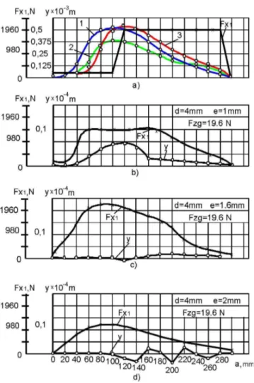
Figure 4 Objective functions and changes of tensile force Fx1 in relation to the machining length obtained in the case of various

(16)

The results of modelling (Fig. 3 b, c, d) indicate the possibility of obtaining, determined by the process conditions, low values of elastic deformations as a result of controlling the force Fx1, but

with relation to the condition (24) in such cases it is advisable to control Fx1 at given values of

ec-centricity e when testing model 4 (Martos, 1975).

To achieve the required low value of deformation the eccentric tension can be applied (model 4 at e ≠ 0).

Analysis of the results of numerical studies, obtained from relations (23), (24) and (25), as well as the supporting experimental tests, demonstrated that elastic deformations of low-rigidity shafts under eccentric tension control decrease, in the case of the parts class considered, from 2- to 20-fold, and in the case of shafts with d < 6 mm the decrease is achieved at lower values of the tensile force. It was demonstrated that eccentric tension very effectively reduces the elastic deformations of shafts with d≥ 6 mm (_L = 300 mm) as compared to axial tension. For example, at _d = 8 mm,

L = 300 mm, Fp = 147 N, λ1 = Fp/Ff = 0.5 (κr = 900) and values of Fx1 = 980 N, e = 2.5 mm (Fig.

4d) elastic deformations on the whole machining length are from 2- to 2.4-fold lower than in the case of axial tension. With adaptive control of the values of eccentricity e and force Fx1, the value of

elastic deformations can be reduced 18-fold; it amounts to (3 – 4.5)·10–2 mm (L = 300 mm, d = 8 mm, Fp = 147 N, λ1 = 0.5, Fx1 = 1245N, e = 7.8 mm) and is practically stable over the whole

length (Fig. 4e).

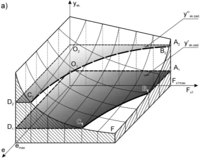
Figure 5 General view of 3D of hyperbololid like shape of the response surface for the values of the objective function – a); relations

of change of objective function y(0), tensile force Fx1 (x) and eccentricity e with relation to length L at x = a – b, c, d,e:

b) (d=6mm, Fzg=49N, Fx10=980N, L=300mm, Ff=30N), c) (d=6mm, Fzg=70N, Fx10=980N, L=300mm, Ff=40N), d)

(17)

Figure 5 (continued)

To determine the optimum parameters Fx1 and e, taking into account the limitations (24), (25),

one can apply both the method of grids and (with relation to the unimodal nature of the objective function) the gradient method.

A general view of the numerically estimated 3D response surface for the objective function (23) with process limitations in the form of Fx1max, emax, and with an extreme at point F is presented in

Fig. 4a. In many cases there is no need to find the extreme, and it is sufficient to determine the required value of ysk.zad. The cutting planes O1A1C1D1 and O2A2C2D2 correspond to the required

values of y’sk.zad. and y”sk.zad., relative to which the set of optimum values of Fx1 and e is sought.

The relations of changes of the objective function y, tensile force Fx1 and eccentricity e at various

shaft diameters and values of machining force, obtained by means of modelling as a result of search with the gradients method, are presented in Fig. 4b,c,d,e. The modelling was conducted with the assumption of the following conditions: d = 6 mm, Fzg = 49 N, Fx10 = 980 N, Ff = 30 N (Fig. 4b);

d = 6 mm, Fzg = 70 N, Fx10 = 980 N, Ff = 40 N (Fig. 4c); d = 8 mm, Fzg = 147 N, Fx10 = 980 N,

Ff = 196 N (Fig. 47d); d = 8 mm, Fzg = 147 N, Fx10 = 980 N, Ff = 196 N (Fig. 4e).

As follows from analysis of the results presented in Fig 4, control of the level of machining accu-racy, at elastic-deformable state of the part with L/d = 15 – 50, can be effected with sufficient ef-fectiveness through the control of two parameters: tensile force Fx1 and eccentricity e; this permits

the achievement of a theoretically assumed level of accuracy.

(18)

5 CONCLUSIONS

To determine the optimum parameters Fx1 and e, taking into account the limitations (24), (25), one

can apply both the method of grids and (with relation to the unimodal nature of the objective func-tion) the gradient method.

References

Altintas Y (2000) Manufacturing automation: metal cutting mechanics, machine tool vibrations, and CNC design. Cambridge: Cambridge University Press.
Bisu CF, K'nevez JY, Darnis P, Laheurte R, Gerard A (2009) New method to characterize a machining system: application in turning. Int J Mat Form 2:93-105.
Bisu CF, Darnis P, Gerard A, K'nevez JY (2009) Displacements analysis of self-excited vibrations in turning. Int J Advanc Manufac Tech 44:1-16.
Cahuc O,K'nevez JY, Gerard A, Darnis P, Albert G, Bisu CF, Gerard C (2010) Self-excited vibrations in turn-ing: cutting moment analysis. Int J Advanc Manufac Tech 47:217‐225.
Cardi AA, Firpi HA, Bement MT, Liang SY (2008) Workpiece dynamic analysis and prediction during chatter of turning process. Mechanical Systems and Signal Processing 22: 1481-1494.
Halas W, Taranenko V, Swic A, Taranenko G (2008) Investigation of influence of grinding regimes on surface tension state. Lecture Notes In Artificial Intelligence, Vol. 5027, Berlin, Heidelberg: Springer - Verlag, pp. 749-756.
Han X, Ouyang H, Wang M, Hassan N, Mao Y (2012) Self-excited vibration of workpieces in a turning process. Proc IMech Part C: J Mech Engin Science 226:1958-1970.
Hassui A, Diniz AE (2003) Correlating surface roughness and vibration on plunge cylindrical grinding of steel, Int J Mach Tools Manufac 43:855-862.
Jianliang G, Rongdi H (2006) A united model of diametral error in slender bar turning with a follower rest. Int J Mach Tools Manufac 46:1002-1012.
Katz R, Lee CW, Ulsoy AG, Scott RA (1988) The dynamic response of a rotating shaft subject to a moving load, J Sound Vibr 122:131-148.
Li CJ, Ulsoy AG, Endres WJ (2003) The effect of flexible-tool rotation on regenerative instability in machining. J Manuf Science Engineer 125:39-47.
Litak G, Rusinek R, Teter A (2004) Nonlinear analysis of experimental time series of a straight turning process. Meccanica 39:105-112.
Litak G, Rusinek R (2012) Dynamics of a stainless steel turning process by statistical and recurrence analyses. Meccanica 47:1517-1526.
Litak G, Kecik K, Rusinek R (2013) Cutting force response in milling of Inconel: Analysis by wavelet and Hil-bert-Huang transforms. Latin American Journal of Solids and Structures 10:133-140.
Martos B (1975) Nonlinear programming. Theory and methods, North-Holland, Amsterdam.
Movahhedy M, Mosaddegh P (2006) Prediction of chatter in high speed milling including gyroscopic effects. Int J Machine Tools Manufacture 46:996-1001.
Ouyang H, Wang M (2007) A dynamic model for a rotating beam subjected to axially moving forces, J Sound Vibr 308:674-682.
Pus VE, Pigert R, Sosonkin VL (1982), Avtomaticeskie stanocnye sistemy, Moscow Masinostroenie.
Qiang LZ (2000) Finite difference calculations of the deformations of multi-diameter workpieces during turning. J Mat Process Technol 98:310-316.
Tlusty J (2000) Manufacturing processes and equipment. Upper Sadde River, NJ: Prentice Hall.
Sen AK, Litak G, Syta A, Rusinek R (2013) Intermittency and multiscale dynamics in milling of fiber reinforced composites. Meccanica 48:738-789.
Świć A, Taranenko V, Wołos D (2010) New method for machining of low-rigidity shafts. Adv Manufac Scien
Technol 34:59-71.
Świć A, Taranenko W, Szabelski J (2011) Modelling dynamic systems of low-rigid shaft grinding. Maintenance
and Reliability 13-24.
Xiong GL, Yi JM, Zeng C, Guo HK, Li LX (2003) Study of gyroscopic effect of the spindle on stability character-istics of the milling system. J Manuf Process Tech 138:379-384.