ISSN 1549-3636
© 2011 Science Publications
Corresponding Author: Ali Ashrafi, Institute for Mathematical Research, University Putra Malaysia, 43400 UPM SERDANG, Selangor, Malaysia Tel: +6017-2940140 Fax:+603-89437958
749
The Efficiency Measurement of Parallel Production Systems:
A Non-radial Data Envelopment Analysis Model
1,2
Ali Ashrafi, 1,3Azmi Bin Jaafar, 1,4
Mohd Rizam Abu Bakar and 1,4Lai Soon Lee 1
Institute for Mathematical Research, University Putra Malaysia, 43400 UPM SERDANG, Selangor, Malaysia
2
Department of Mathematics, Faculty of Mathematics, Statistics and Computer Science, University of Semnan, Semnan, Iran
3
Department of Information Systems,
Faculty of Computer Science and Information Technology, 4
Department of Mathematics, Faculty of Science,
University Putra Malaysia, 43400 UPM SERDANG, Selangor, Malaysia
Abstract: Problem statement: Data Envelopment Analysis (DEA) is a non-parametric technique for measuring the relative efficiency of a set of production systems or Decision Making Units (DMU) that have multiple inputs and outputs. Sometimes, DMUs have a parallel structure, in which systems composed of parallel units work individually; the sum of their own inputs/outputs is the input/output of the system. For this type of system, conventional DEA models treat each DMU as a black box and ignore the performance of its units. Approach: This study introduces a DEA model in Slacks-Based Measure (SBM) formulation which considers the parallel relationship of the units within the system in measuring the efficiency of the system. Under this framework, the overall efficiency of the system is expressed as a weighted sum of the efficiencies of its units. Results: As an SBM model, the proposed model is non-radial and is suitable for measuring the efficiency when inputs and outputs may change non-proportionally. A theoretical result shows that if any unit of a parallel system is inefficient then the system is inefficient. Conclusion: This study introduces a non-radial DEA model, takes into account the operation of individual components within the parallel production system, to measure the overall efficiency as well as the efficiencies of sub-processes. This helps the decision makers recognize inefficient units and make later improvements.
Key words: Data envelopment analysis, decision making unit, production possibility set, parallel production system, slacks-based measure
INTRODUCTION
Data Envelopment Analysis (DEA) is a linear programming methodology in Operations Research and Economics that is extensively applied by various research communities (Sohn and Moon, 2004; Seol et al., 2007; Rayeni and Saljooghi, 2010 Zreika and Elkanj, 2011). The domain of inquiry of the DEA is a set of production systems or decision making units (DMU), which use multiple inputs to produce multiple outputs. The aim of the DEA is to measure the relative efficiency of each DMU within a data set. The results specify how efficient each DMU has performed as compared to other DMUs in converting inputs to outputs. An issue which is of greater concern to the inefficient DMUs is what factors
750 In some situations, DMUs have a parallel structure that is composed of a set of units that work individually; the sum of their own inputs/outputs is the input/output of the DMUs. A typical example of these production systems is a university with faculties. The overall efficiency of the university can be calculated by the total inputs used and total outputs produced by all faculties. Each specific faculty can have an efficiency measured by comparing it with the equivalent faculties of other universities. The study of Färe and Primont (1984), which discusses the efficiency of firms with multiple plants, is probably the first study of such DMUs. Kao (1998) applied the Färe and Primont’s methodology for measuring the efficiency of forest districts with multiple working circles in Taiwan. Castelli
et al. (2004) discussed a hierarchical structure in which if there is only one layer, it becomes a parallel system. The works of Färe et al. (1997), Tsai and Molinero (2002) and Yu (2008) extend of the independent parallel system where certain resources are shared by some units.
Conventional DEA models view this type of production system as a black box and ignore the operations of its units. Recently, Kao (2009) has modified a standard DEA model and introduced a radial DEA model that evaluates the overall efficiency of the system as well as the efficiencies of its units. His method decomposes the inefficiency slack of a DMU into the inefficiency slacks of its sub-DMUs. As an application of Kao’s parallel model, Rayeni and Saljooghi (2010) examine the performance of the universities in Iran via a parallel production process.
This study presents an alternative method for estimating the efficiency of a parallel production system and the efficiency of its units. Since DEA models implicitly use Production Possibility Set (PPS) to evaluate the efficiency of DMUs, we first define the PPS of the parallel production systems. Then, based on this PPS, we introduce a non-radial DEA model in Slacks-Based Measure (SBM) formulation for aggregating the units in a parallel production system. Under this framework, the overall efficiency of the system is expressed as a weighted sum of the efficiencies of its units. With decomposition of the overall efficiency, the units which cause the inefficient operation of the system can be identified for future improvements An example from the forest production industry in Taiwan is applied to compare the new approach with Kao’s parallel model.
MATERIALS AND METHODS
Production possibility set: Suppose we have n DMUs, where each DMUj (j=1,…,n) uses m inputs xij(i = 1, …, m) to produce s outputs yrj(r = 1,…, s). It is assumed
that all inputs and outputs are positive. We denote the DMUj by (xj, yj), where xj = (x1j, x2j,…, xmj)T and yj = (y1j, y2j,…, ymj)T are input and output vectors, respectively. The Production Possibility Set (PPS) T is defined as a set of all inputs and outputs of a production technology in which outputs can be produced from inputs. Under the assumption of Constant Returns to Scale (CRS) the PPS can be represented as follows:
n n
C j j j j j
j 1 j 1
T (x, y) x x , y y , 0, j 1,..., n
= =
⎧ ⎫
⎪ ⎪
=⎨ ≥ λ ≤ λ λ ≥ = ⎬
⎪ ⎪
⎩
∑
∑
⎭where,
λ
=
(
λ
1,...,
λ
n)
∈
ℜ
n is the intensity vector. The PPS under Variable Returns to Scale (VRS) assumption can be defined by adding the convexity constraint∑
nj 1=λ =j 1 into Tc.Definition 1: (Dominance). We say that DMUp (xp, yp) dominates DMUq (xq, yq) if and only if xp≤xq and yp≥yq with strict inequality holding for at least one component in the input or the output vector.
Thus, a DMU of the PPS is not dominated if and only if there is no other DMU (original or virtual) in the PPS which satisfies Definition 1.
Definition 2: (Efficiency). DMUo=(xo,yo) is efficient if and only if there is no (x,y) of PPS such that (x,y) dominates (xo,yo).
Radial and non radial DEA model: DEA provides
for two types of measure: radial and non-radial. Radial models assume proportional change of inputs or outputs and usually disregard the existence of slacks in measuring efficiency scores. Radial measures are represented by CCR (Charnes et al., 1978) and BCC (Banker et al., 1984) Non-radial models, on the other hand, regard the slacks of each input or output and the variations of inputs and outputs as not proportional; in other words in non-radial models the inputs/outputs are allowed to decrease/increase at different rates. Non-radial models include Russell measure (Färe and Lovell, 1978) and Slacks-Based Measure (SBM) (Tone, 2001).
751 free, θ 0, s , s λ, , s y λ y , s x λ θx s.t. ) s s ε( θ min θ n 1 j j j o j n 1 j j o s 1 r r m 1 i i * ≥ − ∑ = + ∑ = ∑ + ∑ − = + − + = − = = + = − (1)
where, ε is non-Archimedean small value and the optimal solution of θ*is efficiency score. Also non-negative vectors s (s ,...,s )1 m m
− − −
= ∈ℜ and
s
1 s
s+=(s ,...,s )+ + ∈ℜ indicate input excess and output
shortfall slacks, respectively. Likewise the output-oriented CCR model can be defined.
Suppose an optimal solution for model (1) to be
* * * *
( ,θ λ ,s ,s )− + .
Definition 3: (CCR-efficiency). DMUo is
CCR-efficient if and only if θ* =1 and s−* = s+*=0.
The model presented in (1) is called the CCR envelopment model. The dual of model (1) (without ε, i.e., ε = 0), or the CCR multiplier model, is given by:
0, v u, n, 1,..., j 0, vx -uy 1, vx s.t. uy max θ j j o o * ≥ = ≤ = = (2)
where, v=(v1,...,vm)∈ℜm and
s s 1,...,u ) (u
u= ∈ℜ
are dual variable vectors corresponding to the constraints of model (1).
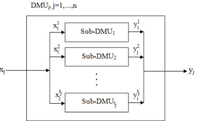
Fig. 1: The parallel production system
The SBM model, as a non-oriented and non-radial DEA model, for evaluating the efficiency of DMUo is defined as follows:
m i i 1 * io s r r 1 ro n
o j j
j 1 n
o j j
j 1
1 s
1
m x
ρ min ρ
1 s
1
s y
s.t. x λx s ,
y λy s ,
λ, s , s 0
− = + = − = + = − + − = = + = + = − ≥
∑
∑
∑
∑
(3)The optimal solution of ρ* is the SBM efficiency score. It can be obviously identified that 0<ρ*≤1 and supports the properties of unit invariance and monotone.
Suppose an optimal solution for model (3) to be
* * * *
( ,ρ λ,s ,s )− + .
Definition 4: (SBM-efficiency). DMUo is
SBM-efficient if and only if ρ* = 1.
This definition is equivalent to s−*=s+* =0. It means that there are no input excesses and output shortfalls in any optimal solution.
The input (output)-oriented SBM model can be defined by ignoring the denominator (numerator) of the objective function.
Here we emphasize that, as demonstrated by Tone (2001), the efficiency score measured by the SBM model is not greater than the efficiency score measured by the CCR model. Moreover, a DMU is SBM-efficient if and only if it is CCR-efficient.
Parallel production system: Consider a parallel production process as shown in Fig. 1. Suppose we have n DMUs, of which each DMUj (j=1,…,n) is composed of tj units (sub-DMUs) connected in parallel. Each sub-DMU uses the same inputs to produce the same outputs, individually. Sub-DMUp (p=1,…,tj) has m inputs
p ij
x (i=1,…,m) and s outputs
p rj
y (r=1,...,s). The sum of all xpij over p, namely,
j p
t ij p 1= x
∑
and the sum of all yprj over p, namely,j p
t rj p 1= y
752 j j p t j j p 1 p t j j p 1
x x ,
y y = = = =
∑
∑
(4)Kao’s parallel model: Kao (2009) has developed a
DEA model based on the input-oriented CCR multiplier model such that by minimizing the inefficiency slack instead of maximizing the efficiency, we are able to decompose the inefficiency slack of a DMU into the inefficiency slacks of its sub-DMUs. Kao’s model for measuring the inefficiency of DMUo is given by:
o t p o p 1 o
o o o
p p p
o o o o
p p
j j j
j j
min s
s.t. vx 1,
uy vx s 0,
uy vx s 0, p 1,...,t ,
uy vx 0, j 1,...,n,j o,p 1,...,t ,
uy -vx 0, j 1,...,n, j o,
u,v 0 = = − + = − + = = − ≤ = ≠ = ≤ = ≠ ≥
∑
(5)where, so and
p
o o
s (p=1,..., t ) are the inefficiency slacks of DMUo and its sub-DMUs, respectively.
On optimality, the efficiency scores for DMUo and sub-DMUp (p = 1,…,to) can be calculated as follows:
o
t
* p*
o o o
p 1 p*
p o
o * p o
o
E 1 s 1 s
s
E 1 , p 1,...,t ,
v x = = − = − = − =
∑
(6)where, (*) shows the optimal value from model (5).
The parallel SBM model: The PPS TCparallel under the CRS assumption for n×tj sub-DMUs of n parallel production systems, is defined by:
j j
t t
n n
parallel p p p p p
C j j j j j
j 1 p 1 j 1 p 1
T (x,y) x λx , y λy , λ 0
= = = = ⎧ ⎫ ⎪ ⎪ =⎨ ≥ ≤ ≥ ⎬ ⎪ ⎪ ⎩
∑∑
∑∑
⎭Note that if all λpj, p=1,..., tj associated with the
sub-DMUs within the DMUj are the same, then
parallel C T
converts to the conventional PPC, namely TC.
Suppose, DMUo (o∈{1,….,n}) to be the DMU under evaluation. In an effort to measure the overall efficiency of DMUo, first by using the input-oriented SBM model, we calculate the efficiency score of each sub-DMUp (p=1,…,to) as follows:
j
j
m
p i
o p
i 1 io t n
p p p
j j o
j 1 p 1 t n
p p p
j j o
j 1 p 1 p
j j
1 s
E min
1-m x
s.t. λx s x ,
λy s y ,
λ, s , s 0, p 1,...,t , j 1,...,n
− = − = = + = = − + = + = − = ≥ = =
∑
∑∑
∑∑
(7)After evaluating the efficiency scores of all Sub-DMUs, we define the overall efficiency score of DMUo as a weighted combination of the efficiency scores of its sub-DMUs. This is shown in the following equation:
o o o
t t t
1 1 2 2 p p
o o o o o o o o o
p 1
E w E w E ... w E w E
=
= + + + =
∑
(8)where, the weight wpo of each sub-DMUp is
p m p
io
o o
i 1 io
1 x
w , p 1,..., t
m = x
=
∑
= (9)Hence wpo is the arithmetic mean of the portion of
resources devoted to each sub-DMU by DMUo. From (4), it can be verified that
o t p o p 1 w 1 = =
∑
.Definition 5: DMUo is said to be efficient in sub-DMUp, if
p o E =1.
Definition 6: DMUo is said to be efficient if its overall efficiency score is equal to one, i.e., Eo=1.
Decomposing the overall efficiency of a system into the weighted combination of its unit’s efficiencies helps us to identify the units that cause inefficiency. By using the model (7), we are able to recognize the inefficient sub-DMUs and make later improvements. Also, using Eq. 8 we can evaluate the overall efficiency of the DMUo in a way that takes into account the operations of all its sub-DMUs.
753 such that the weights associated to sup-DMU of DMUo can be defined as:
p s p
ro
o o
r 1 ro
1 y
w , p 1,..., t
s = y
=
∑
= (10)RESULTS
The following theorem explains the relationship between the efficiency of a parallel production system and its production units.
Theorem 1: If any of sub-DMUp=(x , y ) (ppk pk =1,..., t )k
of DMUk is CRS-inefficient, then DMUk = (xk, yk) is CRS-inefficient.
Proof: Suppose any of sub-DMUp=(x , y )pk pk (p=1,…,tk) to be CRS-inefficient. We will show that there is
parallel C
(x, y)∈T such that (xk, yk) is dominated by (x,y). Without loss of generality, we assume that
1 1
1 k k
sub-DMU =(x , y ) is CRS-inefficient. Then, the
following system has a solution }
s ; s j; , t 1..., p ,
λ
{ pj* = j∀ −* +* with (s−*,s+*)>(0,0):
j
j
t n
1 p* p *
k j j
j 1 p 1 t n
1 p* p *
k j j
j 1 p 1
x λ x s ,
y λ y s
− = =
+ = =
= +
= −
∑∑
∑∑
(11)
We set:
j j
t t
n n
1 1 * p* p 1 1 * p* p
k k j j k k j j
j 1 p 1 j 1 p 1
x x s− x , y y s+ y
= = = =
= − =
∑∑
λ = + =∑∑
λ (12)From (4) and (12) we have
k k
t t
1 p * 1 p *
k k k k k k
p 2 p 2
x x x s , y− y y s+
= =
= +
∑
+ = +∑
− (13)Now we define:
k k
t t
1 p 1 p
k k k k
p 2 p 2
x x x , y y y
= =
= +
∑
= +∑
. (14)Since (x , y )1k 1k ∈PCparallel, thus
parallel C
(x, y)∈T . Hence
we have:
* *
k k
x = +x s , y− = −y s+ (15)
Since (s ,s )−* +* ≠(0, 0), (x , y )k k is dominated by
(x, y). Hence, according to Definition 2, DMUk is
CRS-inefficient.
As a contraposition to Theorem 1, we have.
Corollary 1: If DMUk(xk, yk) is CRS-efficient, then each sub-DMUp=(x , y )pk pk (p=1,…,tk) of DMUk is
CRS-efficient.
Empirical example: Now, we apply the proposed
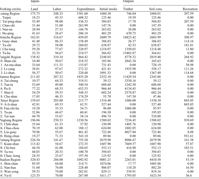
model to the national forests of Taiwan as studied by Kao (2009). In Taiwan, the forest lands are divided into eight regions, each of which is divided into four or five sub-regions called working circles (WCs). These WCs are the basic component in the management of the forest. The forest production process is a characteristic parallel production process, in that each region has several subordinated WCs operating individually. There are four inputs:
• Land (x1): area in thousand hectares • Labor (x2): number of employees in persons • Expenditures (x3): money spent each year in ten
thousand new Taiwan dollars
• Initial stocks (x4): volume of forest stock before the period of evaluation in 10000 m3
• The outputs are
• Timber production (y1): timber produced each year in cubic meters
• Soil conservation (y2): volume of forest stock in 10000 m3, as higher stock level leads to less soil erosion; and
• Recreation (y3): visitors serviced by forests every year in thousands of visits
The data are shown in Table 1. For each input (output) the quantity of a region is the sum of its sub-regions.
754
Table 1: Taiwan forest data
Inputs Outputs
--- --- Working circles Land Labor Expenditures Initial stocks Timber Soil cons. Recreation
Lotung Region 175.73 248.33 1581.60 1604.38 746.04 1604.01 207.59
1. Taipei 18.23 45.33 608.32 125.46 19.59 125.46 0.00
2. Tai-ping-shan 55.49 98.00 336.33 584.85 17.70 584.85 207.59
3. Chao-chi 31.44 51.00 263.99 147.76 0.00 147.39 0.00
4. Nan-au 28.94 27.33 166.78 263.02 38.00 263.02 0.00
5. Ho-ping 41.63 26.67 206.18 483.29 670.75 483.29 0.00
Hsinchu Region 162.81 316.67 850.05 2609.79 16823.42 2603.99 308.97
6. Guay-shan 41.48 86.33 158.49 386.03 26.37 386.03 114.16
7. Ta-chi 29.72 58.00 260.02 638.87 42.53 638.87 181.01
8. Chu-tung 59.28 77.67 220.97 1218.07 1350.65 1214.48 13.80
9. Ta-hu 32.33 94.67 210.57 366.82 15403.87 364.61 0.00
Tungshi Region 138.42 310.34 864.42 2348.03 4778.32 2819.48 264.92
10. Shan-chi 10.40 50.67 218.55 103.86 2842.34 165.63 0.00
11. An-ma-shan 33.64 111.33 153.07 731.43 0.00 728.19 38.98
12. Li-yang 38.01 97.67 272.32 421.41 1935.98 558.17 111.26
13. Li-shan 56.37 50.67 220.48 1091.33 0.00 1367.49 114.68
Nantou Region 211.82 287.32 1835.20 2352.10 11429.54 2343.86 0.00
14. Tai-chung 10.57 64.33 319.51 39.12 3330.16 39.12 0.00
15. Tan-ta 52.69 49.00 340.54 688.60 1242.50 688.60 0.00
16. Pu-li 77.22 68.33 652.53 966.44 4134.43 966.44 0.00
17. Shui-li 54.29 59.33 348.33 602.24 2574.87 602.24 0.00
18. Chu-shan 17.05 46.33 174.29 55.70 147.58 47.46 0.00
Chiayi Region 139.65 203.00 215.77 1316.48 1086.00 1330.10 845.05
19. A-li-shan 42.81 69.33 62.51 527.44 0.00 527.40 845.05
20. Fan-chi-hu 19.28 35.33 54.71 96.00 1086.00 95.97 0.00
21. Ta-pu 32.86 44.67 60.41 196.30 0.00 195.85 0.00
22. Tai-nan 44.70 53.67 38.14 496.74 0.00 510.88 0.00
Pingtung Region 196.06 250.33 1230.56 1588.02 7236.45 1588.02 939.69
23. Chih-shan 35.64 61.33 37.92 150.90 1405.76 150.90 0.00
24. Chao-chou 70.19 62.00 188.12 624.80 1802.85 624.80 0.00
25. Liu-guay 70.96 55.67 461.42 722.46 4027.84 722.46 8.08
26. Heng-chun 19.27 71.33 543.10 89.86 0.00 89.86 931.61
Taitung Region 226.54 141.67 755.20 2679.98 8086.47 2679.98 161.38
27. Kuan-shan 113.42 54.67 272.35 1607.90 7669.57 1607.90 57.87
28. Chi-ben 44.54 41.00 184.65 552.13 416.90 552.13 103.51
29. Ta-wu 44.03 20.33 100.70 394.03 0.00 394.03 0.00
30. Chan- kong 24.55 25.67 197.50 125.92 0.00 125.92 0.00
Hualien Region 320.43 284.00 1092.92 4001.21 2263.01 4410.58 53.19
31. Shin-chan 85.95 64.00 314.71 1074.86 17.77 1085.88 0.00
32. Nan-hua 51.60 76.00 228.40 886.07 110.28 882.20 16.50
33. Wan-yong 59.53 74.00 282.01 829.11 339.91 819.16 0.00
34. Yu-li 123.35 70.00 267.80 1611.17 1795.05 1623.34 36.6
DISCUSSION
As pointed out by many authors including Kao and Hwang (2008), Kao (2009), Chen et al. (2009), Tone and Tsutsui (2009) and Cook et al. (2010), the conventional DEA models apply a single process to evaluate the transforming efficiency of multiple inputs and outputs such that they fail to measure the efforts of different processes and sub-processes within the production systems. Thus, we cannot evaluate the impact of sub-process inefficiencies on the overall efficiency of the system as a whole. In these cases, it is possible that the conventional DEA models evaluate a system as efficient even if none of its component processes is efficient
755
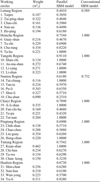
Table 2: Efficiency scores
Working Weight Parallel Conventional
circles (wp
o) SBM model SBM model
Lotung Region 0.4410 0.589
1. Taipei 0.187 0.3050
2. Tai-ping-shan 0.322 0.4840
3. Chao-chi 0.161 0.2960
4. Nan-au 0.136 0.4490
5. Ho-ping 0.194 0.6180
Hsinchu Region 0.7544 1.000
6. Guay-shan 0.216 0.4670
7. Ta-chi 0.229 0.6900
8. Chu-tung 0.334 0.8220
9. Ta-hu 0.221 1.0000
Tungshi Region 0.9110 1.000
10. Shan-chi 0.134 1.0000
11. An-ma-shan 0.272 0.6740
12. Li-yang 0.271 1.0000
13. Li-shan 0.323 1.0000
Nantou Region 0.6180 0.732
14. Tai-chung 0.116 1.0000
15. Tan-ta 0.224 0.5970
16. Pu-li 0.343 0.6350
17. Shui-li 0.227 0.5710
18. Chu-shan 0.090 0.2310
Chiayi Region 0.7890 1.000
19. A-li-shan 0.335 1.0000
20. Fan-chi-hu 0.160 0.4660
21. Ta-pu 0.221 0.4320
22. Tai-nan 0.284 1.0000
Pingtung Region 0.6900 1.000
23. Chih-shan 0.138 0.5710
24. Chao-chou 0.288 0.5880
25. Liu-guay 0.354 0.6260
26. Heng-chun 0.220 1.0000
Taitung Region 0.7542 1.000
27. Kuan-shan 0.462 1.0000
28. Chi-ben 0.234 0.6270
29. Ta-wu 0.154 0.6290
30. Chan- kong 0.150 0.3230
Hualien Region 0.6730 1.000
31. Shin-chan 0.256 0.6280
32. Nan-hua 0.210 0.6100
33. Wan-yong 0.223 0.5700
34. Yu-li 0.311 0.8280
Table 3: Ranking of efficiency scores
Kao’s results
---
Regions Our ranking Ranking Overall efficiency
Lotung Region 8 8 0.752
Hsinchu Region 3 4 0.823
Tungshi Region 1 1 0.937
Nantou Region 7 7 0.773
Chiayi Region 2 2 0.701
Pingtung Region 5 5 0.799
Taitung Region 4 3 0.860
Hualien Region 6 6 0.794
Thus the new approach is suitable for measuring the overall efficiency of the whole system with the added benefit of allowing inefficient sub-DMUs to be identified and potentially rectified.
CONCLUSION
In an earlier study, a radial DEA model was introduced by Kao (2009) for measuring the efficiency of a system composed of parallel units operating independently and where the sum of inputs/outputs for all units is equal to the input/output of the system. In this study, we have introduced a non-radial model based on a Slacks-Based Measure (SBM) framework that evaluates the overall efficiency of the system by considering the operations of its units. Under this framework, the overall efficiency of the system is expressed as a weighted sum of the efficiencies of its units. With decomposition of the overall efficiency, the units which cause the inefficient operation of the system can be identified for future improvements
The proposed model is based on the assumption of Constant Returns to Scale (CRS). By adding the convexity constraint into the PPS which is built by n×tj sub-DMUs, the discussion can be expanded to use the Variable Returns to Scale (VRS) assumption.
It is noteworthy that real systems are generally more complex than the parallel system discussed in this study. Tone and Tsutsui (2009) developed a network DEA model based on a weighted SBM approach that can be applied in series systems. Since the series and parallel structure are two basic structures of a network system, we can transform a network system into a combination of series and parallel structures to evaluate the overall efficiency and the efficiencies of sub-processes.
ACKNOWLEDGMENT
The researchers thank Professor Azizollah Memariani for his comments and suggestions. This work is supported by Graduate Research Assistance of University of Putra Malaysia (Grand no. 5523936).
REFERENCES
Banker, R.D., A. Charnes and W.W. Cooper, 1984. Some methods for estimating technical and scale efficiencies in DEA. Manage. Sci., 30: 1078-1092. DOI: 10.1287/mnsc.30.9.1078
Castelli, L., R. Pesenti and W. Ukovich, 2004. DEA-like models for the efficiency evaluation of hierarchically structured units. Eur. J. Operat. Res., 154: 465-476. DOI: 10.1016/S0377-2217(03)00182-6
756 Chen, Y. and J. Zhu, 2004. Measuring information
technology’s indirect impact on firm performance. Inform. Technol. Manage. J., 5: 9-22. DOI: 10.1023/B:ITEM.0000008075.43543.97
Chen, Y., W.D. Cook, N. Li and J. Zhu, 2009. Additive efficiency decomposition in two stage DEA. Eur. J. Operat. Res., 196: 1170-1176. DOI: 10.1016/j.ejor.2008.05.011
Cook, W.D., J. Zhu, G. Bi and F. Yang, 2010. Network DEA: Additive efficiency decomposition. Eur. J. Operat. Res., 207: 1122-1129. DOI: 10.1016/j.ejor.2010.05.006
Färe, R. and C.A.K. Lovell, 1978. Measuring the technical efficiency of production. J. Econ. Theory,
19: 150-162.
http://ideas.repec.org/a/eee/jetheo/v19y1978i1p150 -162.html
Färe, R. and D. Primont, 1984. Efficiency measures for
multi plant firms. Operat. Res. Lett., 3: 257-260.
Färe, R., R. Grabowski, S. Grosskopf and S. Kraft, 1997. Efficiency of a fixed but allocatable input: A non-parametric approach. Economics Lett., 56: 187-193. DOI: 10.1016/S0165-1765(97)81899-X Kao, C., 1998. Measuring the efficiency of forest
districts with multiple working circles. J. Operat. Res. Society, 49: 583-590. ISSN: 0160-5682
Kao, C. and S.N. Hwang, 2008. Efficiency decomposition in two-stage data envelopment analysis: An application to non-life insurance companies in Taiwan. Eur. J. Operat. Res., 185: 418-429. DOI: 10.1016/j.ejor.2006.11.041
Kao, C., 2009. Efficiency measurement for parallel production systems. Eur. J. Operat. Res., 196: 1107-1112. DOI: 10.1016/j.ejor.2008.04.020 Liang, L., F. Yang, W.D. Cook and J. Zhu 2006. DEA
models for supply chain efficiency evaluation. Annals Operat. Res., 145: 35-49. DOI: 10.1007/s10479-006-0026-7
Rayeni, M.M. and F.H. Saljooghi, 2010. Network data envelopment analysis model for estimating efficiency and productivity in universities. J. Comput. Sci., 6: 1252-1257. DOI: 10.3844/jcssp.2010.1252.1257
Rayeni, M.M. and F.H. Saljooghi, 2010. Benchmarking in the academic departments using data envelopment analysis. Am. J. Applied Sci., 7: 1464-1469. DOI: 10.3844/ajassp.2010.1464.1469 Seol, H., J. Choi, G. Park and Y. Park, 2007. A
framework for benchmarking service process using data envelopment analysis and decision tree. Expert Syst. Appl., 32: 432-440. DOI: 10.1016/j.eswa.2005.12.01
Sexton, T.R. and H.F. Lewis, 2003. Two-stage DEA: An application to major league baseball. J. Productivity Anal., 19: 227-249. DOI: 10.1023/A:1022861618317
Sohn, S. and T. Moon, 2004. Decision tree based on data envelopment analysis for effective technology commercialization. Expert Syst. Appl., 26: 279-284. DOI: 10.1016/j.eswa.2003.09.01
Tone, K. and M. Tsutsui, 2009. Network DEA: A slacks-based measure approach. Eur. J. Operat. Res., 197: 243-252. DOI: 10.1016/j.ejor.2008.05.027
Tone, K., 2001. A slacks-based measure of efficiency in data envelopment analysis. Eur. J. Operat. Res., 130: 498-509. DOI: 10.1016/S0377-2217(99)00407-5
Tsai, P.F. and C.M. Molinero, 2002. A variable returns to scale data envelopment analysis model for the joint determination of efficiencies with an example of the UK health service. Eur. J. Operat. Res., 141: 21-38. DOI: 10.1016/S0377-2217(01)00223-5 Yu, M.M., 2008. Measuring the efficiency and return to
scale status of multi-mode bus transit-evidence from Taiwan’s bus system. Applied Econ. Lett., 15: 647-653. DOI: 10.1080/13504850600721858 Zreika M. and N.Elkanj, 2011. Banking efficiency in