Dielectric Lens Antennas
Carlos A. Fernandes, Instituto de Telecomunicações, Instituto Superior Técnico, Universidade de Lisboa, Lisboa, Portugal
Eduardo B. Lima, Instituto de Telecomunicações, Instituto Superior Técnico, Universidade de Lisboa, Lisboa, Portugal
Jorge R. Costa, Instituto de Telecomunicações, Instituto Universitário de Lisboa (ISCTE -IUL), Lisboa, Portugal
ABSTRACT
Dielectric lens antennas are attracting a renewed interest for millimetre- and sub-millimetre wave applications where they become compact, especially for configurations with integrated feeds usually referred as integrated lens antennas. Lenses are very flexible and simple to design and fabricate, being a reliable alternative at these frequencies to reflector antennas. Lens target output can range from a simple collimated beam (increasing the feed directivity) to more complex multi-objective specifications. This chapter presents a review of different types of dielectric lens antennas and lens design methods. Representative lens antenna design examples are described in detail, with emphasis on homogeneous integrated lenses. A review of the different lens analysis methods is performed, followed by the discuss ion of relevant lens antenna implementation issues like feeding options, dielectric material characteristics, fabrication methods and a few dedicated measurement techniques. The chapter ends with a detailed presentation of some recent application examples involving dielectric lens antennas.
KEYWORDS
Lens Antennas, Geometric Optics, Physical Optics, Lens Feeds, Dielectric Materials, Lens Manufacturing, Lens Profile Design, Optimization.
INTRODUCTION
The use of a dielectric lens as part of an antenna is almost as old as the demonstration of electromagnetic waves by Hertz. In fact, in 1888 Oliver Lodge used a dielectric lens in his experiments at 1 m wavelength (Lodge and Howard 1888). However, it was not until World War II that research on lens antennas has progressed further. Lenses were used to transform the radiation pattern of the primary feed into some high gain radiation pattern, either for fixed or scanning beam applications. But at that time they were supplanted by reflector antennas, less bulky and lighter at microwaves.
With the fast advances on the millimetre and sub-millimetre waves circuit technology for the past two decades, there has been a renewed interest on lens antennas, which present a more acceptable size at these frequencies. Lenses are being explored for
imaging applications, for fixed and mobile broadband communications, automotive radar applications, among others. In most cases the target radiation pattern continues to be the collimated beam type (plane wave output) either fixed or scanning. But interesting highly shaped beams conforming to demanding amplitude templates have also been explored.
Lenses can be used to modify the phase or the amplitude (or both) of the primary feed radiation pattern in order to transform it into a prescribed output radiation pattern. In this sense lenses are equivalent to reflectors. However, instead of reflection, the lens operation principle is based on the refraction of electromagnetic waves at the lens surfaces (in the case of isotropic homogenous lenses), or within the lens dielectric material in the case of non-uniform refractive index lenses. For instance in one of its most basic configurations, Figure 1(A), parallel rays of an incident plane wave are refracted at the lens surfaces in such a way that all output rays intersect at a point, the lens focal point. All these rays have the same electrical path length, that is, they arrive in phase at the focal point (Fermat’s principle), despite their different physical lengths which are compensated by a slower phase velocity (v=c/n) in different portions of the lens. In most designs, lens dimensions are large in terms of wavelength enabling the use of quasi-optical design methods. Large lenses share with reflectors its inherent large bandwidth, which is limited only by the feed bandwidth.
(A) (B)
Figure 1 – Focusing antennas: (A) lens; (B) reflector.
One main advantage of lenses over reflectors is that the feed and its supporting structure do not block the antenna aperture. This back feeding feature was key for the development of the millimetre and sub-millimetre wave integrated lens antenna concept where the lens base is positioned directly in contact with the feed, such as an integrated circuit front-end, to produce a directive radiation pattern either single-beam or multiple-beam. The integrated lens structure is very flexible to accommodate demanding output radiation pattern specifications, while multiple shells can be added for instance to increase the design degrees of freedom maintaining a compact structure . This contrasts with multi-reflector systems where blockage issues force large complex structures.
The existence of powerful software simulation tools, numerically controlled machines, 3D additive manufacturing technologies, low-loss dielectric materials and an exploding knowledge on artificial dielectrics are favouring the development and fabrication of very sophisticated high performance lens antennas, namely integrated lens antennas, that
focal length (𝐹) focal point
𝑛>1
focal point
are easily accessible to most laboratories or companies and affordable for mass market products.
MAIN TEXT
1 Lens Theory
This section starts with a brief overview of different types of known lenses and presents a possible classification. This is followed by some basic concepts applicable for quasi-optical lens design, assuming that the lens dimensions and radius of curvature at every point of the surfaces are large compared to the wavelength. Finally this section presents some alternative lens design approaches, involving a combination of iterative algorithms and lens analysis methods.
1.1 Lens types
The lens classification adopted in this Chapter is based on three different physical characteristics: the feed position relative to the lens body (far from the lens or in direct contact), refractive index profile (constant/stepped or non-uniform) and number of refraction surfaces, see Table 1. For each of these categories the lenses can be further classified according to the type of output radiation pattern: fixed-beam (collimated or shaped) or scanning beam (usually collimated).
In early lenses and in few current designs the focal point is located well away from the lens, at a distance comparable with its diameter as in Figure 1(A). These lenses are named in this Chapter the off-body fed lenses and all examples found in the literature are axial symmetric.
Table 1 – Lens classification based on physical characteristics.
1. Off-body fed 1.1 Homogeneous A. Single refraction B. Multiple refraction 2. Integrated
2.1 Homogeneous C. Single refraction D. Multiple refraction 2.2 Non-uniform index E. Continuous refraction
F. Multiple refraction
Figure 2 - Examples of integrated lens antennas.
𝑛 𝑛3 𝑛1 𝑛2 𝑛4 (A) (B)
Lenses can alternatively be designed to have the feed in direct contact with the lens body (or within the body or at a fraction of the wavelength away). These are referenced in the literature as integrated lens antennas (ILA). These lenses can be made with one or more shells although the most common designs use a single layer.
The concept of integrated lenses started with single material hemispherical lenses added on top of integrated circuit antennas to eliminate substrate modes and increase radiation efficiency (Rebeiz 1992). This has evolved to the use of other fixed canonical shapes like the elliptical or extended-hemispherical to further enhance gain, producing collimated output beams (Filipovic 1993).
But the integrated lens configuration is especially flexible to satisfy more el aborate output beam specifications like secant square type of radiation patterns using more complex lens surfaces (Fernandes 1999), which can have an arbitrary 3D shape in the general case to produce non-symmetrical radiation patterns (Bares 2007). In (Fernandes 2001) the lens shape is adapted to transform the radiation of the circular-symmetrical source into an output shaped beam with square or rectangular footprint when pointed at the ground.
Adding a further shell to the integrated lens adds a second refracting surface offering a supplementary degree of freedom to impose another design condition without sacrificing too much the lens compactness, see Figure 3. For instance in (Costa 2008a) a double-shell lens is designed to satisfy both a beam scanning beam condition and maximum power transfer across the lens surfaces.
Figure 3 – Shaped integrated dielectric lens antenna.
The Luneburg lens is a special case of integrated lenses, with non-uniform refractive index, where ideally an incident plane wave is focused on the antipodal point on the lens surface, see Figure 2(B).
1.2 Geometrical Optics for lens design
Geometrical Optics (GO) is a very convenient formulation for lens (or reflector) design. It derives from the asymptotic solution of Maxwell equations in the high frequency limit (Kay 1965). As long as the overall lens dimensions and surface radius of curvature at any point are much larger than the wavelength, wave propagation inside a homogenous isotropic lens may be conveniently modelled in terms of elementary ray tubes. These emanate from the phase centre of the source, see Figure 4, along straight lines, with the amplitude weighted by the radiation pattern of the source and decaying with path length in the inverse proportion of the square root of the tube cross -section, and with phase given by the electrical path length. Reflection and transmission at an interface are
𝑛𝑠𝑢𝑏𝑠
𝑛1
𝑛2 integrated
made according to Snell’s laws (which derive from the Fermat’s principle), and ray amplitude is affected by Fresnel coefficients and a divergence factor.
Figure 4 – Geometry of the lens and ray tube for GO formulation.
Assuming that the interface between two dielectric media can be considered locally plane, the reflection of an incident plane wave occurs in the same medium, with equal incident and reflected angles – Snell’s law for reflection. The refraction is governed by the following Snell’s law:
𝑛1sin(𝜃𝑖𝑛𝑐) = 𝑛2sin(𝜃𝑡𝑟𝑎𝑛𝑠) (1)
where n1 and n2 are the refraction indexes of each medium and inc and trans are the
incidence and transmission angles defined with respect to the interface normal, see Figure 5. If the two media present the same magnetic permeability of air (most of the usual lens materials do), then 𝑛1 = √𝜀𝑟1 and 𝑛2= √𝜀𝑟2 where 𝜀𝑟1 and 𝜀𝑟2 are the
relative electric permittivity of each media. The refracted wave is bent towards the surface normal if the wave enters a medium with higher dielectric constant, see Figure 5(A), and it is bent away from the normal when exiting a medium with higher dielectric constant, see Figure 5(B).
(A) (B)
Figure 5 – Plane wave incident at an interface between two dielectrics; (A) incidence from the lower index medium; (B) incidence from the higher index media.
𝜂 𝐢Ƹ 𝜑 𝐧ෝ 𝐭Ƹ 𝑧 𝑦 𝑛1 𝑛2 𝑑𝑆 𝑑𝑆′ 𝑥 𝜃 𝜃𝑡𝑟𝑎𝑛𝑠 P 𝜃 𝑖𝑛𝑐 𝜃𝑟𝑒𝑓 = 𝜃𝑖𝑛𝑐 𝑛1 𝑛2> 𝑛1 𝜃𝑡𝑟𝑎𝑛𝑠 < 𝜃𝑖𝑛𝑐 P’ 𝜃𝑡𝑟𝑎𝑛𝑠 𝜃𝑖𝑛𝑐 𝜃𝑟𝑒𝑓 = 𝜃𝑖𝑛𝑐 𝑛1 𝑛2 < 𝑛1 𝜃𝑡𝑟𝑎𝑛𝑠 > 𝜃𝑖𝑛𝑐 P’ P
In the general case the lens surface has an arbitrary curved shape, although with large curvature radius (compared to the wavelength) at any point, and so it is convenient to present the equation (2) in a more general form:
(𝑛1 𝐢Ƹ − 𝑛2 𝐭Ƹ)×𝐧ෝ = 0 (2)
where 𝐢Ƹ and 𝐭Ƹ represent the incident and refracted wavenumber directions, respectively (see Figure 4) and 𝐧ෝ represents the surface normal. By expressing these three unit vectors in spherical coordinates centred at the feed phase centre, equation (2) for an axial symmetric lens takes the form:
𝑑𝑟 𝑑𝜂 =
𝑛2 𝑟 sin(𝜃 − 𝜂)
𝑛1 − 𝑛2 cos(𝜃 − 𝜂) (3)
where 𝑟(𝜂) represents the unknown lens profile while the output angle function 𝜃(𝜂) is the other unknown to be specified by some design condition involving phase, or amplitude or eventually polarization. This condition may be given by an algebraic equation or by a differential equation. The simultaneous equations must be integrated in the interval 𝜂 ∈ [0, 𝜂𝑚𝑎𝑥] with applicable initial conditions 𝑟(0) and 𝜃(0) and final
value 𝜂𝑚𝑎𝑥. This integration is usually performed numerically, taking only a few seconds to provide the final lens shape.
If other dielectric interfaces are involved in the ray paths, each one must conform to its Snell’s equation equivalent to (3). Additional interfaces allow the enforcement of additional radiation pattern specifications which translate into corresponding equations involving the radius 𝑟𝑛(𝜂) of the 𝑛𝑡ℎ interface and the ray exit angle 𝜃𝑛(𝜂). The system
of all the involved equations is solved by generalizing the procedure described above for the single interface. It is noted however that the formulation is different for spherical lenses like the Luneburg or Maxwell fish-eye lenses where the unknown function is no longer 𝑟(𝜂). The refractive index profile 𝑛(𝑟) is the unknown function in these lenses. These type of lenses are not the main focus of the present chapter and are treated as specific cases ahead.
The characterization of multiple internal reflections becomes intricate with the increase in the number of lens shells, but in general there is no significant advantage in including its effect in the lens synthesis process. The design formulation must include however the transmission coefficients, divergence factor and material dissipation losses where applicable. Internal reflection analysis can be performed a posteriori when evaluating the lens performance.
Because of lenses large dimensions in terms of wavelength, dissipation losses are also an important aspect to mind. The material permittivity is a complex valued function of the form 𝜀𝑟(1 − 𝑗 tan 𝛿) where the imaginary part inside the parenthesis is the loss
tangent. A spherical wave propagating inside the lens material has the form
𝐸0(𝜃, 𝜑)𝑒
−𝑗2𝜋√𝜀𝑟(1−𝑗 tan 𝛿)𝑟𝜆
𝑟
(4)
So the total dissipation loss depends on lens dimensions, its shape and feed illumination function. For low loss materials, loose bounds for the dissipation loss in a homogeneous lens can be calculated for the minimum and maximum radius 𝑟 of the lens using
𝐿 = 27.3√𝜀𝑟
𝑟
𝜆tan 𝛿 [𝑑𝐵] (5)
Considering that typical lens radius that copes with the Geometrical Optics approximation range from 10 to 30 , a value of tan = 10-3 corresponds to dissipation
losses ranging from about 0.4 to 1.3 dB.
A simple procedure to verify the lens design is to perform a ray tracing, by shooting rays from the feed point at equal angular intervals and using Snell’s laws to trace the rays’ propagation inside and outside the lens, see Figure 6. This can reveal for instance the shape of the output phase front, phase centre position or the existence of caustics. The lens radiation pattern in the optical limit can be easily obtained by representing throughout the solid angle the ratio 𝑑𝑆/𝑑𝑆′ of the ray tubes defined in Figure 4, weighted by the feed radiation pattern.
Figure 6 – Ray tracing in a secant squared lens antenna example with embedded feed. GO based lens synthesis has been used in the literature for different design specifications ranging from simple phase correction problems (Olver 1988) or with additional aperture taper specification, to multi-beam or beam-scanning problems (Kelleher 1961), or to stringent beam-shaping problems (Fernandes 1999). It has been applied for axis-symmetrical lens synthesis as well as for any arbitrary shaped lens (Salema 1998; Fernandes 2001; Sauleau 2006; Bares 2007), for multiple-shell lenses (Silveirinha 2000), for non-uniform refractive index lenses (Cornbleet 1994), or, in fact, for any combination of the previous cases.
The exact solution for the generic 3D structures using GO is numerically involved, but feasible (Salema 1998; Sauleau 2006; Bares 2007). Perturbation methods like the one proposed in (Fernandes 2001) may be simpler to implement for specific types of non-symmetrical target radiation patterns and it allows to find the appropriate shape for the required non-symmetrical lens. In this reference the lens shape is adapted to transform the radiation of the circular-symmetrical source into an output shaped beam with square or rectangular cross section. An adaptation of the same principle can be used to adjust the lens shape to produce an axis-symmetrical output beam.
1.3 Other lens design methods
The advantage of the direct GO synthesis method presented in the previous section is that it provides the lens shape that satisfies the design requirements after elementary
numerical evaluation of closed form analytical expressions, without the need for any trial and error iterations. Required memory and CPU resources are really modest in the case of axial symmetric lenses. Although the direct GO synthesis is enough for a large number of applications, the method is asymptotic, valid in the optical limit thus neglecting diffraction effects that become important as the lens size reduces.
Alternative lens design methods can be considered when a more accurate lens solution is required for given specifications. They are typically based on a trial and error process involving a parameterized lens model and a lens performance analysis method. The accuracy of the design depends on the accuracy of the numerical modelling and number of required iterations, conditioned by available computational resources. The efficiency of the design process depends very much on how smart the optimization procedure is, due to lens-specific issues which are detailed ahead. Using the direct GO synthesis lens as the first guess for the iterative process may enhance its efficiency.
Before describing the alternative iterative lens design method, it is worth summarizing the following concepts:
A closed-form lens synthesis method (like the GO method described in the previous section) starts from a list of input parameters and design specifications and directly provides an appropriate lens shape based on a closed form formulation, without the need for trial and error iterations. In this sense this can be further classified as a direct synthesis method. In general the verification of the lens performance requires the subsequent single-time use of a lens analysis method.
In iterative lens synthesis methods the lens shape is described by some analytical or numerical representation with unknown coefficients which are determined inside an iterative optimization cycle that tests each generated lens using an appropriate lens analysis method until the target specifications are met by trial and error.
A lens analysis method is intended to evaluate the performance of an existing lens either using an approximate method or a full-wave solver. Its output is the lens performance, not the lens shape.
Unlike direct synthesis methods, the list of available analysis methods is considerably larger. The most used are presented in Table 2, grouped according to the type of electromagnetic modelling. A brief description of these methods is provided in Section 2.
Table 2 - Possible lens antenna analysis methods.
Approximate
Geometrical Optics / Physical Optics (GO/PO) Physical Optics / Physical Optics (PO/PO)
Spectral Domain Method (SDM)
Full Wave
Spherical Wave Modal Method Finite Element Method (FEM)
Method of Moments (MoM) Finite-Difference Time-Domain (FDTD)
Figure 5 presents a schematic diagram of the two mentioned approaches for lens design – the direct synthesis method on the left and the iterative synthesis methods on the right. Naturally both start from the definition of the target specifications, lens material and primary feed characteristics. The path on the left provides a fast first guess of the solution, which can be enough for certain problems or can be fed for refinement through the iterative process on the right.
Two alternative approaches are considered for the parametric modelling of the lens. A polynomial type representation can be adopted, where the coefficients are the unknowns to be optimized in the loop instead of the large collection of the lens surface coordinates. This solution is very flexible allowing the representation of arbitrary shapes. The disadvantage is that the optimization algorithm may generate an unnecessary number of useless lenses, not because the geometry is impossible (it can be checked before starting the lens analysis and removed from the test population) but because randomly generated lenses can easily originate total internal reflection, surface wave modes and caustics, especially for integrated multiple-shell lenses which can only be detected after the analysis process.
In the second approach (Lima 2008), the search space can be narrowed to specific classes of lenses by using the analytical lens profiles from the GO synthesis method, but letting the involved parameters be managed by the optimization algorithm. The analytical-based solutions ensure the electromagnetic viability of all the solutions tested in the iterative process. There is a convergence time versus design flexibility trade-off between these two approaches.
The described procedures and the workflow presented in Figure 7 are implemented in a freeware lens design, analysis and optimization tool – the ILASH software tool (Lima 2008). It was developed for circular symmetric shaped integrated lens antennas with single or double layer, and can handle multiple target specification definitions. The lens analysis method is based on the GO/PO and the optimization is based on genetic algorithms. A screenshot of the ILASH user interface is presented in Figure 8. It allows simple interaction with the kernel, to generate and manipulate lens design data, to fully characterize the lens performance and to export and import results. It is also possible to monitor in real time several aspects of the optimization process like the cost func tion value, lens parameter evolution and convergence. ILASH was used to design the lens examples described in Section 3.
Figure 7 – Block diagram of lens design steps.
Figure 8 – Screenshot of the user interface of the freeware ILASH software.
2 Lens Design, Fabrication and Test
This section presents a few representative examples of lens design, organized according to the lens classification introduced in Section 1. In most of the cases the design is based on GO formulation. The section includes also a discussion of the steps that follow the lens design towards fabrication and test.
Spline lens profiles Parameterized analytical lenses
Input
Lens Synthesis
Lens Analysis
Optimization
Output
Feed characteristics Materials Design Specifications Lens profile Analytical lens profilesLens performance evaluation Diagnostics tools
Optimization algorithm Cost function
2.1 Off-body fed lens design examples
Early works on dielectric lens antennas were based upon the concepts of optical lenses. Most of the late 1800 and early 1900 tests were conducted with off-body fed lenses which were used to collimate the radiation of a plane wave into the feed placed at the focal point in the opposite side of the lens. Also most off-body fed lenses have an axial symmetric shape and, at least during design, the feed radiation pattern is considered also circularly symmetric. These assumptions remove the dependence of the lens with the angle, the angle of rotation about the antenna axis of symmetry. Off-body fed lens antennas are usually made of a single material and can have either one or two refracting surfaces.
2.1.1 Single refraction lenses
The simpler lens configurations with a single refracting surface are the elliptical and the hyperbolic lenses, see Figure 9. In an elliptical lens the surface closer to the feed (inner surface) has a spherical shape and does not refract the rays. The collimation of the rays is achieved from the elliptical surface farther away from the feed (outer surface). In a hyperbolic lens the refraction occurs in the hyperbolic lens surface closer to the feed. In this configuration the outer lens surface is planar and does not refract the rays.
(A) (B)
Figure 9 – Off-body fed lens examples. (A) Elliptical lens; (B) Hyperbolic lens. The shape of the outer surface of the elliptic lens in polar coordinates can be obtained by imposing the path length collimation condition:
𝑟1 + 𝑛 𝑙(𝜂) + 𝑠(𝜂) = 𝑟1+ 𝑛 𝑇 (6)
and the following physical length condition:
[𝑟1 + 𝑙(𝜂)] cos(𝜂) + 𝑠(𝜂) = 𝑟1 + 𝑇 (7)
where 𝑇 is the lens selected thickness at the axis. Subtracting the two equations and noting that 𝑟1+ 𝑙(𝜂) = 𝑟2(𝜂) and that 𝑟1+ 𝑇 = 𝐹 where 𝐹 represents the lens focal
distance, the outer surface profile is expressed as:
𝑟2(𝜂) =𝐹(𝑛 − 1) 𝑛 − cos 𝜂 (8) 𝜂 𝑛 𝑟1 𝑟2(𝜂) focal length (𝐹) focal point 𝑠(𝜂) 𝑙(𝜂) 𝑇 𝜂 𝑛 𝑟1(𝜂) focal length (𝐹) focal point
where 𝑛 is the refraction index of the lens material and F is the lens focal distance. Snell’s equations are implicitly satisfied by the collimation condition (which translates Fermat’s principle).
The inner shape of the hyperbolic lens can be obtained using a similar set of equations and is defined by
𝑟1(𝜂) =𝐹(𝑛 − 1)
cos 𝜂 − 1 (9)
Note that the design is based solely on phase considerations, assuming a point source. In the ideal case when both lenses types with identical diameters are fed with a point source, the elliptical lens presents higher directivity and lower side lobe levels. In fact, all the inner surface points of the elliptical lens are at the same distance from the source and are illuminated with identical amplitude. The main disadvantage of the elliptical lens is that the reflection at the inner surface of the lens, due to the contrast between the air and the dielectric permittivity, is normal to the spherical surface and is reflected back towards the feed (Piksa 2011). In the hyperbolic lens, the diffraction effects at the edges of the lens tend to influence more the main beam of the radiation pattern and increase the side lobe level (Piksa 2011). The hyperbolic lens however may be simpler to manufacture since it presents one planar surface.
2.1.2 Double refraction lenses
Lenses with two refracting surfaces allow more control of the radiation pattern characteristics as discussed in Section 1.2. In fact, based upon geometric optics a set of differential and linear equations can be obtained to determine the coordinates of one of the surfaces (Silver 1984). However, those equations are not sufficient to determine uniquely both surfaces so another design condition must be imposed.
One interesting use for the extra degree of freedom provided by the second refracting surface is in scanning beam applications. If the feed in the previous elliptical or hyperbolic lenses is shifted off the focus on a plane normal to the lens axis, the beam tilts linearly for very small shifts and with a more complex dependence for larger shifts along with increasing beam deformations. In fact the phase front of the output beam is no longer plane for off-axis feed positions. Expanding it in Taylor series reveals a linear term responsible for the linear tilt and non-linear terms responsible for different types of superimposed beam deformations (Born 1959).
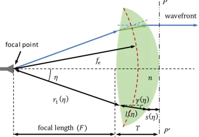
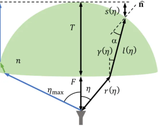
It is possible to extend the linear tilt angle range for scanning beam applications by imposing the so called Abbe sine condition for the design of the second available lens refracting surface. This enables designing a collimating lens which is free from comma aberration when the feed is transversely displaced away from the lens axis (Born 1959). The inner surface of the lens can be defined by the unknown function r1() and the outer
surface by the unknowns length l() and angle () represented in Figure 10. The lens focal length is F and the axial thickness is T. The Abbe sine condition is verified when the intersections of the extended r1() rays departing from the lens focal point and the
corresponding extended transmitted s() rays all lie over an arc of circumference with a certain radius fc centred at the focal point. This is represented by the thick dashed line
in Figure 10. In view of the geometry presented in Figure 10, the Abbe sine condition can be written as
(𝑓𝑒− 𝑟1) sin(𝜂) = 𝑙 sin(𝛾) (10) The Snell’s law at the inner surface of the lens implies that (equation (3))
𝑑𝑟1
𝑑𝜂 =
𝑛 𝑟1sin(𝛾 − 𝜂)
1 − 𝑛 cos(𝛾 − 𝜂) (11)
In order that the electrical path length of every ray is the same at the exiting wavefront, it is required that
𝑟1 + 𝑛𝑙 + 𝑠 = 𝐹 + 𝑛𝑇, (12)
𝑠 + 𝑟1 cos(𝜂) + 𝑙 cos(𝛾) = 𝐹 + 𝑇 (13)
Equations (10)-(13) can be solved simultaneously for 𝑟1(𝜂), 𝑙(𝜂), 𝑠(𝜂) and 𝛾(𝜂) taking 𝜂 as the independent variable and the initial conditions 𝑟1(0) = 𝐹, 𝑙(0) = 𝑇, 𝑠(0) = 0
and 𝛾(𝜂) = 0. The outer surface of the lens can be calculated from the previous four functions.
Figure 10 – Geometry of a two refracting surface lens for Abbe sine condition enforcing. 2.1.3 Zoning
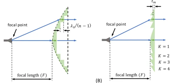
Usually lenses are several wavelengths thick, particularly near the lens axis. For microwave applications this may lead to a very bulky antenna and originate non-negligible dissipation losses in the dielectric. To attenuate those effects, rings of material with a thickness equal to an integer multiple of the wavelength can be removed from the lens, a process called zoning. Figure 11 shows an example for the hyperbolic lens discussed in section 2.1.1 with four zones (K = 4). A minimum physical lens thickness tm
needs to be maintained in the zoned lens to provide structural support, as indicated in Figure 11. The thickness of the zoned lens is independent of the number of zones K and it is given by tm+0/(n-1), which for the example in Figure 11 represents about a quarter
of the original lens thickness.
𝜂 𝑛 𝑓𝑒 𝑟1(𝜂) focal length (𝐹) focal point 𝑠(𝜂) 𝛾(𝜂) 𝑙(𝜂) wavefront 𝑇 P P’
(A) (B)
Figure 11 – Zoning of a hyperbolic lens (A) Original outer hyperbolic shape; (B) Corresponding zoned lens.
The downside of zoned lens is the associated frequency dependence which becomes more important as the lens diameter increases and more zones are used. A criteria to estimate the bandwidth of zoned lenses is given by (Silver 1984): under uniform aperture distribution and lens aperture phase error smaller than 𝜋 4⁄
Bandwidth ≈ 25%
𝐾 − 1 (14)
If the zoning is performed in the non-refracting surface of the lens, shadowing losses can appear at the transition regions and this effect is stronger for lenses with larger ratios between the focal length and the lens diameter F/D (Petosa 2000).
2.2 Integrated lens design examples
This section addresses briefly two classical examples of non-uniform refractive index lenses – the Luneburg lens and the Maxwell fish-eye – and focuses more on the homogeneous shaped lenses. Other non-uniform refractive index lenses have gained also interest with the recent advances in the fields of transformation optics and metamaterials but these exceed the scope of this chapter.
Homogeneous integrated lenses are very effective for integration with low cost millimetre wave circuits, allowing low form-factor solutions with sophisticated radiation pattern characteristics owing to the great design flexibility this lens configuration provides. However, internal reflections may critically influence the lens performance and must be properly analysed in each design. This section presents some representative design examples of canonical lenses as well as some more recent shaped lenses based on GO.
2.2.1 Non-uniform index spherical lenses
In the classical non-uniform spherical lenses the dielectric constant of the material has only radial variation. Therefore, the lens is symmetric in relation to any axis passing the centre of the lens. As a consequence, these spherical lenses do not present a unique focal point but rather a spherical surface concentric with the lens where the focal point can be located depending on the direction of the incident wave.
𝜆0⁄(𝑛 − 1) focal length (𝐹) focal point focal length (𝐹) 𝑡𝑚 𝐾 = 4 𝐾 = 1 𝐾 = 2 𝐾 = 3 focal point
The most known of the spherical lenses is the Luneburg lens (Luneburg 1943) where the lens material permittivity profile varies with the square of the r distance from the lens centre
𝜀𝑟(𝑟) = 2 − (𝑟 𝑅⁄ )2
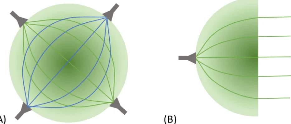
(15) being R the outer radius of the lens. This formulation results in a focal region located at the outer surface r = R of the lens. Therefore, a point source located at any point of the lens surface originates a collimated beam in the opposite direction, Figure 12. This property is independent of the lens diameter. The Luneburg lens is particularly adequate for multi-beam applications since the symmetry ensures that all beams are equal independent of the feed position on the lens surface.
Figure 12 – Luneburg lens with darker colour representing increasing permittivity. Luneburg did not have the opportunity to demonstrate such antenna experimentally since no suitable lens materials were available at the time. Nowadays, Luneburg lenses are formed by discrete number of concentric dielectric layers that approximate the ideal permittivity law of equation (15). It is expected that as the number of discrete layers increases the performance of the lens improves; however, the manufacturing complexity increases as well as the influence of possible air gaps between the layers (Kim 1998). It has been demonstrated that a quite small number of shells is enough to obtain a directivity and side lobe level close to the ideal case (Fuchs 2007). Nevertheless, the recommended number of discrete layers increases with the lens diameter compared to the wavelength. For example, just 6 layers were required to achieve adequate performance with an 80 diameter Luneburg lens (Fuchs 2007a). Even lesser number of
layers is possible by optimizing both the permittivity and thickness of the layers (Mosallaei 2001; Boriskin 2011).
There are also examples of Luneburg lenses fabricated from a single material with controllable dielectric constant. For instance in (Min 2014) a 3D rapid prototyping machine was used to achieve the desired permittivity value by controlling the filling ratio of a polymer/air-based unit cell. Alternatively, it is possible to use foam material and press it to obtain the desired dielectric constant. In fact, when the pressure increases and the foam is compacted, the quantity of air in the material decreases increasing the permittivity. This technique has been tested for the fabrication of a Luneburg lens in (Bor 2014). It is also possible to control the dielectric constant in the Luneburg lens by
drilling holes into the material and varying either the diameter of the holes or their density (Sato 2002; Xue 2007).
One of the major disadvantages of the Luneburg lens is its high profile. Transformation optics (Do-Hoon 2010) can be used to change the shape of the lens into a much lower cylindrical profile. However, common solutions end up resulting in materials that are anisotropic and/or must have relative permeability different than unity forcing the use of metamaterials that are usually narrowband, lossy, dispersive and sometimes cumbersome to manufacture. A reasonable performance has been achieved with a compacted Luneburg lens with cylindrical geometry, formed by discrete layers with step permittivity variation along the radius and along the height (Mateo-Segura 2014). Although a height reduction was obtained, permittivity values as high as 12 are required, and the structure presents some scanning loss.
A commonly used solution to reduce the profile of the Luneburg lens by a factor of 2, is to combine half of the lens with a flat ground plane, Figure 13. The ground plane creates an image of the upper hemisphere and simulates the complete Luneburg lens. The size of the ground plane must be adequate to produce the required image, and the necessary dimensions are function of the elevation angle of the beam in relation to the ground plane. An insufficient ground plane size will reduce the directivity of the beam and cause scanning loss. This hemispheric lens solution also suffers from feed blockage for high elevation angles. One advantage of this configuration is that it is easier to mechanically stabilize than the complete spherical lens. Recently a quarter Luneburg lens with a 90 degree corner ground plane has been demonstrated (Nikolic 2012).
Figure 13 – Half hemisphere Luneburg lens.
A similar configuration to the Luneburg spherical lens is the cylindrical one, Figure 14, where the variation of the dielectric constant occurs only in the radial direction. In this solution the beam collimation is obtained only in one plane, leading to fan shaped beams instead of pencil like beams (Komljenovic 2010).
(A) (B)
Figure 14 – Cylindrical Luneburg lens.
Another classical non-uniform index spherical lens is the Maxwell’s fish-eye lens, which pre-dates the Luneburg lens (Maxwell 1860). The dielectric constant of the lens material is given by
𝜀𝑟(𝑟) = ( 4
[1 + (𝑟 𝑅⁄ )2]2) (16)
where R is the outer radius of the lens. When a point source is placed on the surface of the lens, the radiation is focused at the antipodal point of the lens as represented in Figure 15(A). Due to the lens symmetry, the source radiation is converted into a local plane wave at the centre of the lens. Therefore, if the Maxwell’s fish-eye lens is cut in half it can be used as a collimating lens that focuses a plane wave into a focal point on the surface of the lens, which becomes unique in this case, Figure 15(B). The halved Maxwell’s fish-eye lens (HMFE) has lower profile than the Luneburg lens and is easier to flush mount. Practical implementation of the HMFE has been done using a few discrete layers (Fuchs 2006) and the performance was shown to be comparable with the Luneburg lens when the feed is centred with the lens (Fuchs 2008).
(A) (B)
Figure 15 – (A) Maxwell fish-eye lens; (B) Half Maxwell fish-eye lens. The darker colour represents higher values of permittivity.
Unlike the Luneburg lens, the HMFE lens loses interest for scanning beam applications since scanning losses appear as the feed is moved over the lens surface (Fuchs 2007b). 2.2.2 Elliptical and hemispherical lenses
The homogeneous elliptical integrated lens, just like its off-body fed counterpart treated in Section 2.1.1, is used to transform the radiation pattern of a feed placed at the focal point of the lens into a plane wave in the air medium, propagating along the lens axis,
𝑛1
𝑛2
Figure 16. It can be viewed as the limit when 𝑟1 tends to zero in equations (6)-(7) from Section 2.1.1:
𝑛 𝑟(𝜂) + 𝑙(𝜂) = 𝑛 𝐹 (17)
Also the following physical length condition can be imposed:
𝑟(𝜂) cos 𝜂 + 𝑙(𝜂) = 𝐹 (18)
Eliminating l() between the two equations leads to the same elliptical lens profile found in Section 2.1.1:
𝑟(𝜂) =𝐹(𝑛 − 1)
𝑛 − cos 𝜂 (19)
It is a simple matter to show that this corresponds in rectangular coordinates to
(𝑥 𝑎) 2 + (𝑧 − 𝐿 𝑏 ) 2 = 1 (20)
where a is the radius along the x-axis, b is the radius along the z-axis, L is the position of the focal point in relation to the centre of the lens and 𝑏 + 𝐿 = 𝐹, Figure 16(A). The eccentricity of the elliptical lens is related to the dielectric constant of the material. The following relations hold (Filipovic 1993)
𝑏 = 𝑎
√1 − 1/𝑛2 (21)
𝐿 = 𝑏 𝑛⁄ (22)
The value of a is chosen to define the lens size, and consequently the aperture size required to achieve a certain directivity of the beam.
(A) (B)
Figure 16 – (A) Design variables of an elliptical integrated lens antenna; (B) rays reflection inside the lens.
Only the rays that hit the lens surface above the plane of maximum waist PP’ are focused, Figure 16(B). The feed radiation intersecting the lens below the maximum waist are not collimated but rather propagate along undesired directions or excite surface wave modes (Pasqualini 2004) giving rise to side lobes or other perturbations in the lens
𝑛 𝐹 𝑙(𝜂) 𝑟(𝜂) a b L maximum-waist P 𝜂 P’ 𝑛 𝐹2 𝐹1
radiation pattern. For this reason, proper feed configurations should be used to minimize the illumination of the lower part of the lens surface.
Internal reflections may be especially critical in integrated lens antennas. For instance if the feed is at the centre of an hemispherical lens, all reflected rays travel back along the same path of the corresponding incident rays, concentrating at the focal point, usually causing a substantial mismatch at the feed impedance. A similar effect occurs in the elliptical lens; all reflected rays concentrate at the feed point after travelling through the second focal point of the elliptical lens, originating a second order reflection at another point of the lens surface, Figure 16(B). (Neto 1998; Neto 1999; Van Der Vorst 1999; Van Der Vorst 2001). Again, this causes feed impedance mismatch. Part of the second order ray is transmitted to the air at an undesired direction causing side lobes in the lens radiation pattern. These undesired effects increase with the contrast between the material and the air refraction indexes. For other integrated lens shapes the reflected rays may not be all reflected back into the feed, nevertheless, they may be responsible for transmission of higher than first order rays along undesired directions, reducing the main beam efficiency or causing ripple.
The problem of internal reflections can be tackled, at least within a limited bandwidth. For normal incidence on a planar interface between two dielectric media with refraction index 𝑛1 and 𝑛2, it is possible to cancel the reflected ray by adding an appropriate
intermediate layer, Figure 17(A). Its dielectric refraction index 𝑛𝑚𝑎𝑡𝑐ℎ must be 𝑛𝑚𝑎𝑡𝑐ℎ = √𝑛
1𝑛2 (23)
and a thickness h
ℎ =
𝜆
04
𝑛𝑚𝑎𝑡𝑐ℎ (24)where 0 is the free space wavelength. This intermediate layer is usually called the
matching layer.
(A) (B)
Figure 17 – Matching layer (A) in a planar dielectric air interface. The intensity of ray color is proportional to the wave power density; (B) in an elliptical integrated lens
antenna
By adding a matching layer to the lens surface it is possible to alleviate the effect of internal reflections, Figure 17(B). It is a fact that the rays do not hit the lens surface along
𝑛 𝑚 𝑎 𝑡𝑐 ℎ h 𝑛1 𝑛2 h 𝑛1 𝑛2 𝑛𝑚𝑎𝑡𝑐ℎ
the normal direction and therefore the thickness of the matching layer should not be given by (24). Instead it should vary along the surface of the lens according to the ray incident angle. In a study presented in (Van Der Vorst 1999) for an elliptical integrated lens of silicon (r=11.7) it was demonstrated that there is no major improvement on the
lens radiation performance by using the optimum thickness matching layer. Therefore, a constant thickness layer given by (24) is generally used, facilitating the manufacturing process. Because it is not easy to find natural materials with specific permittivity values, it is common to synthesize an effective medium layer by periodically removing a fraction of the dielectric material from the lens surface, such as drilling holes or cutting groves (Ngoc Tinh 2010).
The matching layer thickness is frequency dependent and, therefore, reduces the bandwidth of the lens antenna. To improve the bandwidth multiple consecutive matching layers can be used performing a gradual transition between the two dielectric constants at the interface (Ngoc Tinh 2009).
The extended hemispherical lens is another classical configuration of integrated lens, owing to its simple shape for fabrication. It consists of a half sphere of radius R with a cylindrical extension of height L. The feed is located at the base of the lens, Figure 18(B).
(A) (B)
Figure 18 – Extended hemispherical integrated lens antenna: (A) synthesized elliptical; (B) hyper hemispherical.
If the length of the cylindrical extension is chosen to be
𝐿 = 𝑅
𝑛 − 1 (25)
most of the spherical part of the hyper hemispherical lens coincides with an elliptical lens, Figure 18(A). This lens is usually called synthesized elliptical lens (Filipovic 1993) although it tends to present a slightly lower directivity when compared to a true elliptical lens with the same diameter.
A second type of extended hemispherical lens is the hyper hemispherical (Rebeiz 1992) where the cylindrical extension length is
𝐿 = 𝑅 𝑛⁄ (26)
For this particular type of lens the output beam is not collimated, presenting a much broader (and sometimes multi-lobed) radiation pattern when compared to an elliptical lens with the same radius. Nevertheless, the hyper hemispherical lens bends the rays radiated by the feed toward the axis of the lens, Figure 18(B). The lens sharpens the
𝑅 𝐿 𝑛 𝑅 𝐿 𝐷 virtual focus 𝑛
radiation pattern, effectively increasing the gain of the feed by a factor 𝑛2 (Rebeiz 1992). However, unlike collimated lenses, the directivity of this lens does not increase with lens size (or aperture size).
The hyper hemispherical lens satisfies the Abbe sine condition (Born 1959). Therefore, this lens is free from comma aberration when the feed is transversely displaced within certain limits away from the lens axis. This type of lens is particularly useful for beam scanning applications. Another interesting characteristic of hyper hemispherical lenses is that all the rays transmitted into the air focus in a virtual point behind the lens at a distance
𝐷 = 𝑅𝑛 (27)
from the centre of the spherical part of the lens. This means that the radiation pattern of this lens presents a very stable phase centre position coincident with this virtual focus and its position does not shift with the frequency (in the optical limit).
There are several other types of shaped dielectric integrated lens antennas with profiles not given by canonical expressions like the elliptical and extended hemispherical lenses. In section 3 of this chapter several design and implementation examples of non-canonical shaped lenses will be given in more detailed.
2.2.3 Lens designed to match an output power template
Integrated lenses can also be used to conform the output radiation pattern to some far-field power template G(). The formalism of a GO-direct synthesis method is described for an axial-symmetric single material lens with refraction index 𝑛, fed on-axis at the base of the lens as shown in Figure 19 (Fernandes 1999).
Figure 19 – Geometry of a single-shell lens.
The lens design requires the knowledge of the feed power pattern U() when the feed is inside the lens material. This can be obtained using a full-wave analysis of the feed radiating into an unbounded medium with the same permittivity as the lens. Alternatively it can be obtained experimentally using the procedure described in Section 2.7.
The unknown lens profile is represented by the 𝑟(𝜂) function. As before, the Snell’s equation for refraction at the dielectric interface is written as:
x z 𝑛 𝜃(𝜂) 𝜂 𝑟(𝜂) 𝐹
𝜕𝑟 𝜕𝜂=
𝑟(𝜂) sin(𝜃 − 𝜂)
𝑛 − cos(𝜃 − 𝜂) (28)
In order to enforce the output power pattern template, the elementary ray tube concept introduced in Section 1.2 is used, Figure 4. Power conservation in the elementary ray tube is expressed as 𝑈(𝜂)𝑇 sin 𝜂 𝑑𝜂 = 𝐾𝐺(𝜃) sin 𝜃𝑑𝜃 (29) or rearranging 𝑑𝜃 𝑑𝜂 = 𝑇 𝐾 𝑈(𝜂) 𝐺(𝜃) sin 𝜂 sin 𝜃 (30)
where 𝑇(𝜂) represents the transmissivity, that is, the ratio of the power 𝑃𝑡 transmitted
across 𝑑𝑆 to the incident power 𝑃𝑖 (Figure 4). 𝑇 = 𝑈∥|𝑡∥ 2| + 𝑈 ⊥|𝑡⊥2| 𝑈 1 𝑛 cos 𝛽 cos 𝛼𝑇 (31) cos 𝛼 = 𝐢Ƹ ∙ 𝐧ෝ (32) cos 𝛽 = 𝐭Ƹ ∙ 𝐧ෝ (33)
where t// and t represent the Fresnel transmission coefficients for parallel and
perpendicular polarization respectively. 𝐾 is a normalization constant to be determined from the balance between the total power inside the lens and total power outside the lens 𝐾 = ∫ 𝑇(𝜂)𝑈(𝜂) sin 𝜂 𝑑𝜂 𝜂𝑚𝑎𝑥 0 ∫𝜃𝑚𝑎𝑥𝐺(𝜃) sin 𝜃 𝑑𝜃 0 (34)
being 𝜂𝑚𝑎𝑥 the maximum feed aperture and 𝜃𝑚𝑎𝑥 the maximum output angle.
The unknowns 𝑟(𝜂) and 𝜃(𝜂) are obtained by integrating the system of equations formed by (28) and (30) from 𝜂 = 0 to 𝜂𝑚𝑎𝑥 (typically 90°) using the initial condition 𝑟(0) = 𝐹 and 𝜃(0) = 0. 𝐹 acts as a scaling factor, not affecting the lens shape. However, the larger is this value the larger is the lens size. Inherent to the design, increasing the size also improves the lens radiation pattern compliance with the target G().
Function 𝑇(𝜂) in equations (28)-(31) depends indirectly on the unknown function 𝑟(𝜂). An iterative process can be adopted, repeating successively the integration of (28) and (30) considering 𝑇(𝜂) = 𝑐𝑜𝑛𝑠𝑡𝑎𝑛𝑡 in the first step. The obtained solution 𝑟(𝜂) can then be used to calculate 𝑇(𝜂) for the next evaluation of (28)-(31), and the process is repeated until convergence; usually two or three iterations are enough.
The presented formulation assumes independent feed and target template power patterns 𝑈(𝜂) and 𝐺(𝜂). In most cases the feed radiation pattern is not axial symmetric, but an approximation can be generated as an average of the co-components in the main planes for the lens synthesis purpose.
2.2.4 Frequency stable radiation pattern and phase centre position
This section presents the design of a double-shell axial symmetric lens that complies with two design conditions: a well-defined phase centre located behind the lens (outside its body) and a target far-field amplitude template (Fernandes 2010). This type of virtual
focus lens can be useful as reflector primary feed as it will be discussed in the applications section ahead. Lens dimensions are assumed to be large relative to the wavelength, so direct GO synthesis will be used for the lens design.
Considering the geometry from Figure 20, n1 and n2 are the refraction indexes from the
inner and outer lens shells, respectively, and S and F are the corresponding axial depths. The lower value of the refraction index is used at the outer shell to favour lower reflections at the air interface. The two lens surfaces are defined by the unknown functions r1(), () and R() and are obtained by solving a system of three differential
equations as explained next.
Figure 20 – Geometry for the lens design.
One of the equations derives from the power conservation condition in an elementary ray tube crossing the lens system, the same discussed in Section 2.2.3.
𝑑𝜃 𝑑𝜂 =
𝑇(𝜂)𝑈(𝜂) sin 𝜂
𝐾𝐺(𝜃) sin 𝜃 (35)
where 𝑈(𝜂), 𝐺(𝜃), 𝑇(𝜂) and 𝐾maintain the previous definition. Further imposing Snell law for refraction at the inner interface results in (equation (3))
𝑑𝑟1 𝑑𝜂 = 𝑟1(𝜂) sin(𝛾 − 𝜂) 𝑛1 𝑛2 − cos(𝛾 − 𝜂) (36)
while imposing the Snell law at the outer interface results in 𝑑𝑅 𝑑𝜂 = 𝑑𝑅 𝑑𝜃 𝑑𝜃 𝑑𝜂= 𝑅𝑛2sin(𝛾 − 𝜃) 1 − 𝑛2 cos(𝛾 − 𝜃) 𝑇(𝜂)𝑈(𝜂) sin 𝜂 𝐾𝐺(𝜃) sin 𝜃 (37)
Finally, the following path length conditions are imposed:
x z 𝜂 𝛾(𝜂) 𝑟1(𝜂) 𝑛1 𝑛2 𝑙(𝜂) 𝜃(𝜂) 𝜃(𝜂) 𝑅() S F z0
{ 𝑟1𝑛1+ 𝑙𝑛2 = 𝑅
𝑅 cos 𝜃 = 𝑟1cos 𝜂 + 𝑙 cos 𝛾 + 𝑧0 (38)
The lens profile is obtained by solving the system of three differential equations (35), (36) and (37) with respect to integrating from = 0 to = max. The angle required
in (36) and (37) is obtained from the following explicit expression derived from (38)
𝛾 = cos−1[𝑛2(𝑅 cos 𝜃 − 𝑟1cos 𝜂 − 𝑧0)
𝑅 − 𝑛1𝑟1
] (39)
The initial conditions at = 0 are:
{ 𝜃 = 0 𝑟1 = 𝐹 𝛾 = 0 𝑙 = 𝑆 𝑅 = 𝑛1𝐹 + 𝑛2𝑆 (40)
The distance from the phase centre to the base of the lens z0 is settled once the lens
shells refraction index and axial depths are chosen. In fact, from (40) one has
𝑧0 = 𝑅(𝜂 = 0) − 𝐹 − 𝑆 = 𝐹(𝑛1− 1) + 𝑆(𝑛2− 1) (41) Equation (35) is numerically undetermined at = 0. To obtain its value at = 0, the following relation is written from
∫ 𝐾𝐺(𝜃) sin 𝜃 𝑑𝜃 = ∫ 𝑇(𝜂)𝑈(𝜂) sin 𝜂 𝑑𝜂 𝜂 0 𝜃 0 (42)
and evaluated in the limit as 𝜃 → 0 and 𝜂 → 0. The result is
𝜃 = √𝑇(𝜂)𝑈(𝜂)
𝐾𝐺 (𝜃) 𝜂 (43)
where T(), U() and G() are assumed constant near = 0 and = 0. Finally, from the above equation, the corresponding limit value for (35) is given by
𝑑𝜃 𝑑𝜂 = √
𝑇(𝜂)𝑈(𝜂)
𝐾𝐺(𝜃) (44)
This result is also used in the related part of (37) for = 0.
The GO lens synthesis is inherently broadband as long as lens dimensions are large compared to the wavelength and as long as the feed radiation pattern remains constant and coincident with the used U() template.
2.2.5 Multi-beam lens
An integrated lens configuration, formed by two embedded shaped shells, can be designed for multi-beam or scanning applications (Costa 2008a). The possibility to shape two lens surfaces enables that two independent design goals can be specified (in a single-material lens only one design goal can be defined):
A beam collimation condition, i.e., the output rays emerging from the lens are required to be parallel to each other;
A condition that minimizes aberrations of the output beam for off-axis feed positions.
The lens geometry is presented in Figure 21. The structure is axial-symmetric, formed by two embedded shells of different materials; the inner shell presents the higher refraction index value n1 and the outer shell the lower value, n2. An array of feeds is
distributed at the planar base of the lens within a small area centred with the lens axis.
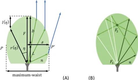
Figure 21 – Geometry for the lens design.
The inner lens surface is defined by the (unknown) function r() and the outer lens surface is defined by the (unknown) length l() and angle () (Figure 21). The lens axial thickness is F and T for the inner and outer shells, respectively.
It is well known that a lens satisfying the so called Abbe sine condition is free from comma aberration for a small off-axis transversal displacement of the feed (Born 1959). The Abbe sine condition is verified when the intersection points of the extended r() rays departing from the on-axis feed and the corresponding extended transmitted s() rays all lie over an arc of circumference with a certain radius fe centred at the sensor
(Born 1959). This is represented by the thick dashed arc in Figure 21. In view of the geometry of Figure 21, the Abbe sine condition can be written as
(𝑓𝑒− 𝑟) sin 𝜂 = 𝑙 sin 𝛾 (45)
Snell’s law at the inner interface implies that 𝑑𝑟
𝑑𝜂 =
𝑟(𝜂) sin(𝛾 − 𝜂) 𝑛1
𝑛2− cos(𝛾 − 𝜂) (46)
In order that the optical path length of every ray is the same at the exiting wavefront, it is required that:
𝑛1𝑟 + 𝑛2𝑙 + 𝑠 = 𝑛1𝐹 + 𝑛2𝑇 (47)
𝑠 = 𝐹 + 𝑇 − 𝑟 cos 𝜂 − 𝑙 cos 𝛾 (48)
Equations (45)-(48) can be solved simultaneously to determine both the inner and the outer shell profiles, taking as the independent variable. The initial condition for = 0 is r = F, l = T and = 0 and the integration is extended up to = edge, where generally
x z 𝛾(𝜂) 𝜂 𝑟(𝜂) 𝑛1 𝑛2 𝑙(𝜂) 𝑠(𝜂) 𝑓𝑒 wavefront F T P P’
edge</2. The calculation is stopped at the point where the outer shell intersects the fe
circle or where the total internal reflection condition is reached.
For a given combination of n1, n2, F and T values, the fe parameter can be adjusted
between F and F+T to control the shape of the lens surfaces (and indirectly the lens scanning characteristics). In the optical limit, the lens shape obtained with the above GO-based formulation is independent of the absolute dimensions, and thus, for instance F, can be taken as a scaling factor.
It is noteworthy that, in line with the classical Abbe formulation for single material lenses (Born 1959), the above design equations consider only the central feed. The imposed Abbe condition implicitly determines the scanning behaviour for off-axis feeds.
2.2.6 Beam steering lens
In the traditional approach for mechanical beam steering, the primary feed is displaced over the focal arch of the focusing element (lens or reflector) originating a corresponding beam tilt. Alternatively the feed can be fixed and the lens (or reflector) tilted in such a way that its focal arch passes always through the feed. Phase errors in the aperture increase with the off-axis feed position originating progressive beam degradation. These become unacceptable typically beyond 25° beam tilt (notable exception is the Luneburg lens, Section 2.2.1).
This section presents an alternative approach where the axis for lens tilting is coincident with the lens focus and consequently coincident with the feed phase centre, Figure 22 (Costa 2009). In this way phase errors associated with the lens tilting are eliminated and in principle larger beam scanning range can be reached, provided that proper illumination of the lens is maintained for all lens tilt angles. The feed remains stationary. An application example of this lens is presented in Section 3.2.4.
Figure 22 – Working principle of the beam steering lens.
A collimated beam lens is used for this concept so, by definition, all output rays emerge always parallel to the lens symmetry axis, making the beam tilt angle coincident with the lens tilt angle. The azimuth beam scanning is obtained by simultaneous rotation of the lens about the feed axis.
𝑛 lens azimuth rotation axis fixed feed lens rotation axis lens symmetry axis
Of course in this case the feed cannot be in contact with the lens. But the system is designed to have the feed as close to the lens base as possible (in the order of one wavelength) to favour proper lens illumination for all lens tilts. Issues to consider when designing the collimated beam lens are the maximum achievable beam tilt angle, the maximum gain and the minimum gain scan loss. Thes e characteristics are determined by the lens profile, but they are in part limited by reflections at the dielectric interfaces and by feed illumination spill over as lens tilt increases. An appropriate feed must be designed for proper lens illumination.
This is a case where numerical optimization is required for the lens design. However, instead of brute force optimization of a spline representation of the lens, an alternative hybrid approach is considered (Section 1.3) where GO design equations are combined with a parametric representation of the lens base surface to narrow the search space. The two refraction surfaces of the lens must be designed maximizing the portion of the output lens surface that is able to collimate the feed’s radiation. This is equivalent to maximize the lens max value defined in Figure 23. The two lens surfaces play a role to
broaden this maximum angle.
Figure 23 – Geometry for the design of the beam steering lens.
The lens geometry is shown in Figure 23. Using Snell refraction law at the bottom lens interface leads to
𝜕𝑟(𝜂)
𝜕𝜂 =
𝑟(𝜂) 𝑛 𝑠𝑖𝑛(𝛾 − 𝜂)
1 − 𝑛 𝑐𝑜𝑠(𝛾 − 𝜂) (49)
where is the independent variable. On the other hand, by imposing an electrical path length condition, one gets
𝑟 + 𝑛 𝑙 + 𝑠 = 𝐹 + 𝑛 𝑇 (50)
where
𝑠 = 𝐹 + 𝑇 − 𝑟 cos 𝜂 − 𝑙 cos 𝛾 (51)
F and T are input constants, whereas r(), l() and () are unknown functions. A third design condition is required to define a unique solution. For that r() is analytically written as a Taylor series expansion in
𝑇 𝛾(𝜂) 𝜂 𝑟(𝜂) 𝑛 𝑠(𝜂) 𝐹 𝑙(𝜂) 𝜂max 𝐧ෝ
𝑟(𝜂) = ∑ 𝐶𝑛
8 𝑛=0
𝜂𝑛 (52)
So the left-hand side of equation (49) can also be written analytically. The following values are set C0=F and C1=0 in order to impose 𝜕𝑟 𝜕𝜂 = 0⁄ at = 0. This ensures null
refraction for the central ray. Coefficients C2 to C8 are generated by using the genetic
algorithm (GA) optimization method. Setting the Cn coefficients defines the r() function
in (52) so () can be calculated from (49) and then l() can be calculated from (50) and (51). The latter functions define the lens upper surface.
As mentioned, the above formulation is integrated with a GA loop to test different shapes of the bottom lens surface r(), with the goal to maximize the max angle of the
lens, subject to the following constraints:
a) r() must be large enough to ensure that the edges of the feed never touch the bottom lens surface when the lens is tilted;
b) The bottom lens surface cannot cross the upper surface except at the edge of the lens;
c) Ray incidence angle at the upper lens interface must be below 95% of the critical angle c.
This latter constraint minimizes the excitation of a lateral wave (Pasqualini 2004) along the lens upper surface. This can happen when ray’s incidence angle , measured with respect to lens local normal 𝐧ෝ, approaches the total reflection condition
𝛼𝑐 = 𝑎𝑠𝑖𝑛(1 𝑛⁄ ) (53)
As previously referred, the surface wave tends to deflect part of the lens radiation away from the main beam direction reducing the directivity.
2.3 Lens analysis methods
2.3.1 Geometrical Optics / Physical Optics (GO/PO) analysis method
The hybrid GO/PO method is certainly the most used approach for lens (reflector and other open structure) analysis. It takes as input the lens shape and material permittivity, the feed position, and the far-field pattern radiated by the feed when immersed in an unbounded media that has the same permittivity as the lens. The GO/PO procedure involves two steps, as implied by the acronym.
In the first step, GO formulation, as explained in Section 1.2 is used to compute the field distribution at the inner face of the lens interface; Fresnel coefficients are then used to compute the fields at the outer face of the lens. When one or more dielectric interfaces are crossed by the ray tubes originated at the feed phase centre, appropriate Fresnel coefficients and divergence factors must be used.
From the field distribution obtained in the first step, equivalent currents are calculated over the outer face of the lens, and these are Kirchhoff-Huygens (KH) integrated over the lens aperture S to provide the lens far-field radiation pattern:
𝐄(𝑃) =𝑗𝑒 −𝑗𝑘𝑅 2𝜆𝑟 ∫ [𝑍(𝐧ෝ×𝐇(𝑃′))×𝐑1+ (𝐧ෝ×𝐄(𝑃′))]×𝐑1𝑒 −𝑗𝑘𝛒∙𝐑1𝑑𝑆 𝑠 (54)
E(P') and H(P') represent the field produced by the feed over the lens outer surface,
calculated in the first step. R1 is a unit vector directed from the origin towards the
observation point P, is a vector directed from the origin towards the integration point P' on the lens surface, and 𝐧ෝ is the outward normal to the lens surface. This second step is referred in the literature as the Physical Optics (PO) integration.
Figure 24 – Geometry for the PO aperture integration.
The GO/PO approach provides very good results for most large aperture antenna problems, provided that the accuracy of the aperture field description is also good. While in the GO direct synthesis approach discussed in the previous section it is enough to consider only the forward propagating rays to define the aperture fields (as already discussed), in the analysis process all the multiple reflected and transmitted rays must be properly accounted. Reference (Ling 1986) proposes a general procedure for tracing the rays in complex arbitrarily shaped structures in the context of radar cross -section problems, which is referred as the Shoot and Bounce Ray method (SBR). The SBR method was used for computation of the internally reflected rays in an integrated elliptical lens (Neto 1998) or in an off-axis feed extended hemispherical lens (Pavacic 2006).
The computation time for the GO/PO method becomes really insignificant when structures are axial-symmetric. Even if the source fields are not axial-symmetric, an appropriate decomposition of those source fields in terms of a series of azimuthal harmonics may transform the non-symmetrical problem into a superposition of solutions for axial-symmetrical problems.
Memory requirements for the GO part of the procedure are reasonably modest, especially for circular-symmetric structures. A similar comment is valid in general also for the PO part of the procedure, having in mind that in some approaches the far-field pattern can be calculated as the superposition of the sequentially calculated closed-form KH-integrations of all exit ray tube fields.
2.3.2 Physical Optics / Physical Optics (PO/PO) analysis method
This is again a two-step analysis method, like the previously studied GO/PO, but now the calculation of the aperture fields in the first step is based on the PO formulation. This allows circumventing two GO limitations:
o GO cannot be used in the first step for small lenses, where the feed can no longer
be accurately represented by a point and by its far-field radiation pattern;
𝜌 𝐧ෝ 𝑅1 𝑧 𝑦 𝜇1, 𝜀1 𝜇0, 𝜀0 𝑉 𝑥 𝑃 𝑂 𝑆 𝑀ഥ𝑆= −𝐧ෝ×(𝐻ഥ) 𝐽ҧ𝑆= 𝐧ෝ×(𝐸ത) 𝑅 𝑃′