Braz. J. Chem. Eng. vol.27 número3

(1)

ISSN 0104-6632 Printed in Brazil

www.abeq.org.br/bjche

Vol. 27, No. 03, pp. 413 - 427, July - September, 2010

Brazilian Journal

of Chemical

Engineering

LEARNING TO REPAIR PLANS AND

SCHEDULES USING A RELATIONAL

(DEICTIC) REPRESENTATION

J. Palombarini

1

and E. Martínez

2*

1_{UTN-Fac. Reg. V. María, Av. Universidad 450, Villa María 5900, Argentina} 2_{INGAR(CONICET-UTN}_),_{Fax: +54 342 4553439.Avellaneda 3657,}

S3002 GJC, Santa Fe, Argentina. E-mail: ecmarti@santafe-conicet.gob.ar

(Submitted: December 12, 2009 ; Revised: July 5, 2010 ; Accepted: July 12, 2010)

Abstract - Unplanned and abnormal events may have a significant impact on the feasibility of plans and schedules which requires to repair them ‘on-the-fly’ to guarantee due date compliance of orders-in-progress and negotiating delivery conditions for new orders. In this work, a repair-based rescheduling approach based on the integration of intensive simulations with logical and relational reinforcement learning is proposed. Based on a relational (deictic) representation of schedule states, a number of repair operators have been designed to guide the search towards a goal state. The knowledge generated via simulation is encoded in a relational regression tree for the Q-value function defining the utility of applying a given repair operator at a given schedule state. A prototype implementation in Prolog language is discussed using a representative example of three batch extruders processing orders for four different products. The learning curve for the problem of inserting a new order vividly illustrates the advantages of logical and relational learning in rescheduling.

Keywords: Automated planning; Artificial intelligence; Batch plants; Reinforcement learning; Relational modeling; Rescheduling.

INTRODUCTION

Most of the existing works addressing schedule optimization in batch plants are based on the assumptions of complete information and a static and fully deterministic environment (Méndez et al., 2006). A pervasive assumption in the deterministic scheduling field has been that the optimized schedule, once released to the production floor, can be executed as planned. However, a schedule is typically subject to the intrinsic variability of a batch process environment where difficult-to-predict events occur as soon as it is released for execution: disruptions always occur and elaborated plans quickly become obsolete (Henning and Cerda, 2000).

Examples of such disruptions include equipment failures, quality tests demanding reprocessing operations, arrival of rush orders and delays in material inputs from previous operations. The inability of most scheduling literature to address the general issue of uncertainty is often cited as a major reason for the lack of influence of current research in the field on industrial practice (Henning, 2009).

(2)

forwards all subsequent activities, (2) rescheduling only a subset of affected operations, or (3) generating an entirely new schedule for all of the remaining tasks. The first method is computationally inexpensive but requires plenty of slack and can lead to poor resource utilization (Herroelen and Leus, 2004). Generating a schedule from scratch maximizes schedule quality, but typically requires a high computational effort and may impose a huge number of schedule modifications (Zhu, et al., 2005). The option of partial rescheduling represents a sort of tradeoff: it aims at the identification of a schedule that provides the optimal combination of schedule efficiency and schedule stability at reasonable computational cost, bearing in mind that rescheduling decisions are taken without too much deliberation on the shop-floor.

Real-time rescheduling is a key issue in disruption management. For example, in refinery supply chains, disruptions such as crude arrival delay could make the current schedule infeasible and necessitate rescheduling of operations. Existing approaches for generating (near) optimal schedules for a real-world refinery typically require significantly large amounts of time. This is undesirable when rectification decisions need to be made in real-time. Furthermore, when the problem data given to the existing scheduling approaches are changed, as is the case during a disruption management scenario, rescheduling may follow different solution paths and result in substantially different schedules. A heuristic rescheduling strategy that overcomes both these shortcomings has been proposed by Adhitya et al. (2007). The key insight exploited in their approach is that any schedule can be broken down into operation blocks. Rescheduling is thus performed by modifying such blocks in the original schedule using simple heuristics to generate a new schedule that is feasible for the new supply chain situation. It is worth noting that rescheduling strategy avoids major operational changes by preserving blocks in the original schedule. The trade-off between performance and stability of the repaired schedule is a very important issue to be addressed.

Fast rescheduling in real-time is mandatory to account for unplanned and abnormal events by generating satisfying schedules rather than optimal ones (Vieira et al, 2003). Reactivity and responsiveness is a key issue in any rescheduling strategy which makes the capability of generating and representing knowledge about heuristics critical for repair-based scheduling using case-based reasoning (Miyashita, 2000). One such example is the CABINS framework for case-based rescheduling proposed by Miyashita and Sycara (1994) that heavily resorts to human experts.

Based on domain-dependent past experience or know-how, evaluation of a repaired schedule in CABINS is done not only from its local and direct effects of repair activities in the resulting schedule, but also on the rather global and indirect influences in the final repaired schedule. Along similar ideas, another important work in the field of the so-called intelligent scheduling techniques are contributions by Zweben et al. (1994). Also, Zhang and Dietterich (1995) applied reinforcement learning to the scheduling problem and succeeded in resorting to repair-based rescheduling in NASA’s space shuttle payload processing problem. Since the objective function in this type of project-oriented rescheduling problems is primarily minimizing makespan, the search for an optimal sequence of repair operators can be conveniently pruned (i.e., the search length is only 20-90 steps).

Schedule repairs in CABINS are based on expert’s predictive capability of global effects of intermediate rescheduling activities. This is a severe limitation of using case-based reasoning in bath plant rescheduling. To overcome the issue of non-existing human experts for domain-specific scheduling problems, integrating intensive simulations with case-based reinforcement learning has been proposed by Miyashita (2000). The tricky issue with this approach is that resorting to a feature-based representation of schedule state is very inefficient and learning is very ineffective and generalization to unseen states is highly unreliable. Futhermore, repair operators are difficult to define in a propositional setting. In constrast, humans can succeed in rescheduling thousands of tasks and resources by increasingly learning a repair strategy using a natural abstraction of a schedule: a number of objects (tasks and resources) with attributes and relations (precedence, synchronization, etc.) among them.

(3)

Learning to Repair Plans and Schedules Using a Relational (DEICTIC) Representation 415

REPAIR-BASED (RE)SCHEDULING

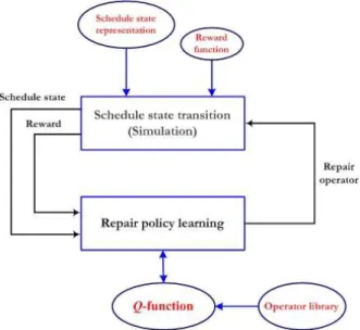
Fig. 1 depicts the repair-based optimization architecture where search control knowledge about repair operator selection is acquired through reinforcements using a schedule state simulator. In the simulation environment, an instance of the schedule is interactively modified by the learning agent using a set of repair operators until a goal is achieved or the impossibility of repairing the schedule is accepted. In each interaction, the learning agent receives information from the schedule situation or state s and then selects a repair operator to be applied to the current schedule, resulting in a new one. The resulting quality of the schedule after the repair operator has been applied is evaluated using the simulation environment via an objective or reward function r(s). The learning agent then updates its action-value function Q(s,a) that estimates the value or utility of resorting to the chosen repair operator a in a given schedule state s. Such an update is made using a reinforcement learning algorithm (Sutton and Barto, 1998) such as the well-known Q-learning rule. By accumulating enough experiences over many simulated interactions, the agent is able to learn an optimal policy for choosing the best repair operator at each schedule state. The main issue for learning is then how schedule states and actions must be represented for knowledge acquisition and iterative revision.

Figure 1: Knowledge acquisition for schedule repair using reinforcement learning.

For repairing a schedule, the agent is given a goal function: goal S → _{{true, false} defining which}

states in the schedule are target states, e.g., states in which total tardiness is less than or equal to 1 working day. The objective of any schedule repair task can be phrased as: given a starting state for the schedule s , find a sequence of repair operators ₁

1 2 n

a ,a ,...,a with a_i∈A such that:

1 1 n

goal( (... (s ,a )...,a ))δ δ =true (1)

where δ is the transition function, which is unknown to the learning agent.

Usually a precondition function pre S×_A →

{true, false} is used to specify which subset of repair operators can be applied at each state of the schedule to account for resource capabilities and precedence constraints (e.g., product recipes). This puts the following extra constraints on the action sequence:

i 1 1 n

a : pre( (... (s ,a )...,a )) true

∀ δ δ = (2)

Also, a reward function is used to approximate a repair policy from reinforcements based on simulations (Martínez, 1999):

t

t t t t t

1 goal(s ) false and

r r(s ,a ) goal( (s ,a )) true

0 otherwise

= ⎧⎪

= =_⎨ δ =

⎪⎩ (3)

A reward is thus only given when a repaired schedule is reached. This reward function is unknown to the learning agent, as it depends on the unknown transition function δ. Based on the reward function and simulation, the optimal policy: a_i= π∗(s )_i can be approximated using reinforcement learning algorithms (Sutton and Barto, 1998; Martínez, 1999). The optimal policy π∗ can be used to compute the shortest action-sequence to reach a repaired scheduled, so this optimal policy, or even an approximation thereof, can be used to improve responsiveness on the shop-floor to handle unplanned events and meaningful disturbances on the shop-floor.

Most research works on reinforcement learning focus on the computation of the optimal utility of states (i.e., the function V∗ or related values) to find the optimal policy π∗. Once this function V∗ is known, it is easy to translate it into an optimal policy. The optimal action in a state s is the action that leads to the state with the highest V*–value:

a

(s) arg max [r(s,a) V ( (s,a))]

∗ ∗

(4)

where 0≤ γ < 1 is a discount factor. As can be seen in equation 4, this translation requires an explicit model of the scheduling world through the use of the state transition function δ (and the reward function r). In rescheduling applications, building such a model of the problem is at least as hard as finding an optimal policy, so learning V∗ is not sufficient to learn the optimal repair policy. Therefore, instead of learning the utility of states V(s), an agent can learn directly a different value Q, which quantifies the utility of an action a in a given state s when following the optimal policy π∗ is used:

Q(s,a)=r(s,a)+ γV ( (s,a))∗ δ (5)

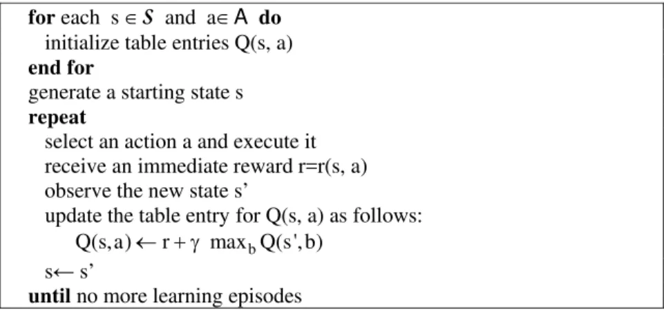
An action in a given state will be optimal if the action has the highest Q-value in that state. A simulation-based algorithm to learn the optimal policy is Q-learning (Watkins, 1989; Sutton and Barto, 1998). Q-learning is a simple algorithm that updates these Q-values incrementally while the reinforcement learning agent interacts with a real or simulated world. Fig. 2 shows a high level description of the algorithm. The value update rule in Q-learning is very simple:

b

Q(s,a)← + γr max Q(s', b) (6)

where s’ is the resulting state of using action a at state s. The key issue in applying reinforcement learning in rescheduling is how a schedule state must be best represented so that the repair policy can be applied to unseen schedule states more effectively. Miyashita (2000) proposed to represent states and actions in a propositional format. This corresponds to describing each state (and possibly each action as well) as a

feature vector with an attribute for some distinctive properties of the schedule state. The features used are the same as the ones used in CABINS, consisting of local and global features. Global features represent information related to the entire schedule, such as total tardiness and total work-in-process in the schedule. Local features are variables that are descriptive of the local schedule in the neighborhood of a given task, milestone or constraint conflict. Propositional representations are not adequate for learning in open planning worlds defined by tasks, their characteristic attributes and their relations to other tasks and resources.

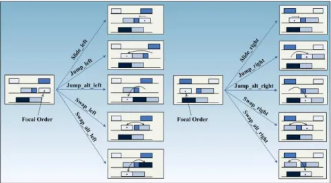
A relational (deictic) representation that deals with the varying number of tasks in the planning world by defining a focal point for referencing objects in the schedule is proposed here as a much powerful alternative. To characterize transitions in the schedule state due to repair actions, a deictic representation resorts to constructs such as:

The first task in the new order.

The next task to be processed in the reactor. Tasks related to the last order.

In a deictic representation, both scheduling states and repair operators (actions) are defined in relation to a given focal point (i.e., a task) as is shown in Fig. 3. These local repair operators move the position of a task alone; however, due to the ripple effects caused by tight resource-sharing constraints, other tasks may need to be moved as well, which is not desirable. Whenever the goal-state for the schedule cannot be achieved using primitive repair operators, more elaborate macro-operators can be used to implement a combination of basic repair operators such as task-swapping, batch-split or batch-merge until a goal state in the repaired schedule (e.g., order insertion without delaying other orders) is achieved.

for each s ∈S_{and a}∈_A_do

initialize table entries Q(s, a) end for

generate a starting state s repeat

select an action a and execute it receive an immediate reward r=r(s, a) observe the new state s’

update the table entry for Q(s, a) as follows:

b Q(s,a)← + γr max Q(s', b) s← s’

until no more learning episodes

(5)

Figure 3: Deictic representations of repair operators.

To gain the most from a deictic representation of states and actions in the rescheduling problem, resorting to a relational interpretation of such relationships, as used in the “learning from interpretations” setting (De Raedt and Džeroski, 1994; Blockeel et al., 1999), is proposed. In this notation, each (state, action) pair will be represented as a set of relational facts.

RELATIONAL REINFORCEMENT LEARNING (RRL)

RRL algorithms are concerned with reinforcement learning in domains that exhibit structural properties and in which different kinds of related objects such as tasks and resources exist (Džeroski et al, 2001; De Raedt, 2008; van Otterlo, 2008). These kinds of domains are usually characterized by a very large and possibly unbounded number of different states and actions, as is the case with planning and scheduling worlds. In this kind of environment, most traditional reinforcement learning techniques break down. One reason why propositional RL algorithms fail is that they store the learned Q-values explicitly in a state-action table, with one value for each possible combination of states and actions. Rather than using an explicit state−action Q-table, RRL stores the Q-values in a logical regression tree (Blockeel and De Raedt, 1998). The relational version of the Q-learning algorithm is shown in Fig. 4. The computational implementation of the RRL algorithm needs to be able to deal successfully with:

the relational format for (states, actions)-pairs in which the examples are represented;

incremental data: the learner is given a continuous

stream of (state, action, Q-value)-triplets and has to predict Q-values for (state, action)-pairs during learning, not after all examples have been processed; a moving target: since the Q-values will gradually converge to the correct values, the function being learned may not be stable during simulation-based learning.

(6)

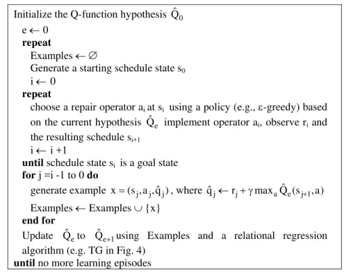
Initialize the Q-function hypothesis Q ˆ₀ e ← 0

repeat

Examples ←∅

Generate a starting schedule state s0

i ← 0

repeat

choose a repair operator ai at si using a policy (e.g., ε-greedy) based

on the current hypothesis Q implement operator aˆ_e i, observe ri and

the resulting schedule si+1

i ← i +1

until schedule statesi is a goal state

for j =i -1 to 0 do

generate example x=(s ,a ,q )_j _j ˆ_j , where ˆq_j← + γr_j max Q (s_a ˆ_e _{j 1}₊ ,a)

Examples ← Examples ∪ {x} end for

Update Q to ˆ_e Qˆ_{e 1}₊ using Examples and a relational regression algorithm (e.g. TG in Fig. 4)

until no more learning episodes

Figure 4: A RRL algorithm for learning to repair schedules through intensive simulations.

Several incremental relational regression techniques have been developed that meet the above requirements for RRL implementation: an incremental relational tree learner TG (Driessens et al., 2001), an instance based learner (Driessens and Ramon, 2003), a kernel-based method (Gärtner et al., 2003; Driessens et al., 2006) and a combination of a decision tree learner with an instance-based learner (Driessens and Džeroski, 2004). Of these algorithms, the TG is the most popular one, mainly because it is relatively easy to specify background knowledge in the form of a language bias. In the other methods, it is necessary to specify a distance function between modeled objects (Gärtner, 2008) or a kernel function is needed between (state, action)-pairs (Driessens et al., 2006).

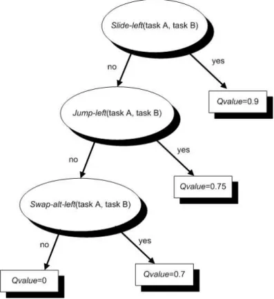
The TG algorithm described in Fig. 5 is a relational regression algorithm that has been developed for policy representation in logical and relational learning (Driessens, 2004; De Raedt, 2008, van Otterlo, 2008). This incremental first order regression tree algorithm is used here for accumulating simulated experience in a compact representation of a repair-based policy based on Q-values for all repair operators available at each state s. Fig. 6 gives a small example of a first order regression tree for the Q-value function in a task (re)scheduling world trained using simulations to react to events and disturbances. A first-order decision tree can be easily translated into a Prolog decision list.

//initialize by creating a tree with a single leaf with empty statistics

for each learning example that becomes available do

sort the example down the tree using the tests of the internal nodes until it reaches a leaf

update the Q-value in the leaf according to the new example if the statistics in the leaf indicate that a new split is needed

then generate an internal node using the indicated test grow 2 new leaves with empty Q statistics end if

end for

(7)

Figure 6: A simple example of a relational regression tree

A first-order decision tree is a binary tree in which every internal node contains a test that is a conjunction of first-order literals. Also, every leaf (terminal node) of the tree contains a prediction (nominal for classification trees and real-valued for regression trees). Prediction with first-order trees is similar to prediction with propositional decision trees: every new instance is sorted down the tree. If the conjunction in a given node succeeds (fails) for that instance, it is propagated to the left (right) subtree. Once the instance arrives at a leaf node, the value of that leaf node is used as the prediction for that instance. TG stores the current tree together with statistics for all tests that can be used to decide how to split each leaf further. Every time an example (triplet) is inserted, it is sorted down the tree according to the tests in the internal nodes and, in the resulting leaf, the statistics of the tests are updated.

EXAMPLE

A small example problem proposed by Musier and Evans (1989) is considered to illustrate the use of repair operators for batch plant rescheduling. The plant is made up of 3 semicontinuous extruders that

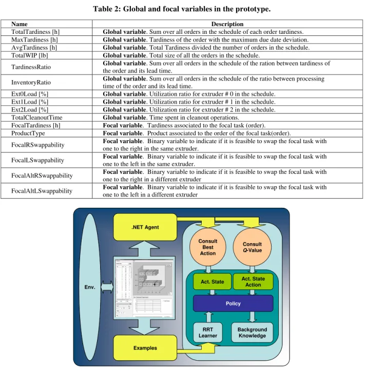
process customer orders for four products. Processing rates and cleanout requirements are detailed in Table 1. Order attributes corespond to product type, due date and size. In this section, this example is used to illustrate concepts like relational definition of schedule states and repair operators, global and focal (local) variables used in the relational model, and the overall process of repairing a schedule bearing in mind minimum increase of the total tardiness when a new order needs to be inserted. In learning to insert an order the situation before the sequence of repair operations is applied is described by: i) arrival of an order with given attributes that should be inserted in a randomly generated schedule state, and ii) the arriving order attributes are also randomly chosen. Variables used to represent scheduled states and repair operators in the relational format are given in Table 2.

The prototype application has been implemented in Visual Basic.NET 2005 Development Framework 2.0 SP2 and SWI Prolog 5.6.61 running under

Windows Vista. The TILDE and RRL modules

from The ACE Datamining System developed by

(8)

Table 1: A small example problem formulation (Musier and Evans, 1989)

Processing rate (lb/day)

A B C D

Extruder #0 100 200 --- ---

Extruder #1 150 --- 150 300

Extruder #2 100 150 100 200

Cleanout requirements (days/cleanout)

Next operation

Previous operation A B C D

A 0 0 0 2

B 1 0 1 1

C 0 1 0 0

D 0 2 0 0

Table 2: Global and focal variables in the prototype.

Name Description

TotalTardiness [h] Global variable. Sum over all orders in the schedule of each order tardiness. MaxTardiness [h] Global variable. Tardiness of the order with the maximum due date deviation. AvgTardiness [h] Global variable. Total Tardiness divided the number of orders in the schedule. TotalWIP [lb] Global variable. Total size of all the orders in the schedule.

TardinessRatio Global variable. Sum over all orders in the schedule of the ration between tardiness of the order and its lead time.

InventoryRatio Global variable. Sum over all orders in the schedule of the ratio between processing time of the order and its lead time.

Ext0Load [%] Global variable. Utilization ratio for extruder # 0 in the schedule. Ext1Load [%] Global variable. Utilization ratio for extruder # 1 in the schedule. Ext2Load [%] Global variable. Utilization ratio for extruder # 2 in the schedule. TotalCleanoutTime Global variable. Time spent in cleanout operations.

FocalTardiness [h] Focal variable. Tardiness associated to the focal task (order). ProductType Focal variable. Product associated to the order of the focal task(order).

FocalRSwappability Focal variable. Binary variable to indicate if it is feasible to swap the focal task with one to the right in the same extruder.

FocalLSwappability Focal variable. Binary variable to indicate if it is feasible to swap the focal task with one to the left in the same extruder.

FocalAltRSwappability Focal variable. Binary variable to indicate if it is feasible to swap the focal task with one to the right in a different extruder

FocalAltLSwappability Focal variable. Binary variable to indicate if it is feasible to swap the focal task with one to the left in a different extruder

Env.

RRT Learner

Examples

Background Knowledge

Policy

Act. State Action Act. State

Consult Q-Value Consult

Best Action .NET Agent

Env.

RRT Learner

Examples

Policy

Env.

RRT Learner

Examples

Policy

(9)

At the beginning of each training episode, the prototype interface asks the user to generate a given number of orders with their corresponding attributes bounded over allowable ranges defined interactively. To generate the initial schedule state s0, these orders

are randomly assigned to one of the three available extruders. Later on, the attributes of the order to be inserted -without increasing the total tardiness in the initial schedule- are generated and it is assigned arbitrarily to one of the extruders. The learning episode progresses by applying a sequence of repair operators until the goal state is reached. At the end of the episode, examples containing the schedule states found during it are archived in the knowledge base “Examples” along with the update made by the induction procedure of the relational regression tree, which resorts to the RRTL (Relational Regression Tree Learner) component of the prototype. This regression tree contains (in relational format) the repair policy learned from “Examples” from the current and previous episodes. Background knowledge, which is valid all over all the domain, is used by the RRTL component (regression tree) to answer queries regarding the Q-value of a given state-action pair or the best repair operator for a given schedule state. These queries are actually processed by the Prolog wrappers ConsultBestAction.exe and ConsultQ.exe, which made up a transparent interface between the .NET agent and the relational repair policy. Also, the RRTL module includes the functionality for discretizing continuous variables such as Total Tardiness and Average Tardiness in non-uniform real-valued intervals, so as to make the generated rules useful for Prolog wrappers. In the .NET application, different classes are used to model Agent, Environment, Actions and Policy using the

files Policy.pl, ActState.pl, ActStateAction.pl and BackgroundKnowledge.pl. Finally, the .NET agent is fully equipped to handle situations where the agent cannot be inserted in the initial schedule. To this aim, the agent may modify order attributes such as date or size so as to insert the order. The prototype allows the user to interactively revise and accept/reject changes made to order attributes to insert it in the initial schedule without increasing the Total Tardiness of the resulting schedule.

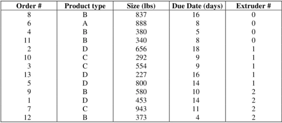
To illustrate the advantages of relational reinforcement learning in order insertion, we consider the specific situation where there exist 10 orders already scheduled in the plant and a new order #11 must be inserted so that the Total Tardiness (TT) in the schedule is minimized. Example data for scheduled orders (#1 through #10) and the new order (#11) in a given episode are shown in Table 3. In each episode, a random schedule state for orders #1 through #10 is generated and a random insertion attempted for the new order (whose attributes are also randomly chosen), which in turn serves as the focal point for defining repair operators. The goal state for the repaired schedule is stated in terms of the TT: a maximum of 5% increase. Background knowledge such as “the number of orders scheduled for extruder #3 is larger than the number for extruder #2” is provided to speed up learning in the relational domain. In Fig. 8, the learning curve for the new order insertion rescheduling event is shown. As can be seen, learning occurs rather quickly in such way that, after 60 episodes, a near-optimal repair policy is obtained. As shown in Fig. 9, the number of repair steps required to reach the goal state is drastically reduced after a few training episodes. After 60 training episodes, only 8 repair steps are required, on average, to insert the 11th order.

Table 3: Example data for the initial orders and the one (# 11) to be inserted.

Order # Product Size [lb] DD [days]

1 A 300 6

2 B 300 5

3 C 700 3

4 D 100 2

5 D 700 10

6 B 600 5

7 A 400 6

8 B 500 12

9 C 700 17

10 C 300 8

(10)

Figure 8: Learning curve for the repair-based order insertion example.

Figure 9: Average number of repair steps to reach the goal state as learning progresses.

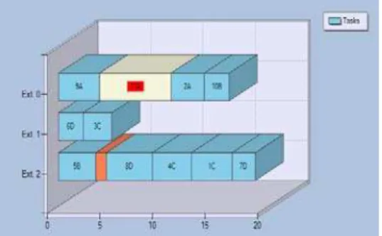
Fig. 10 provides an example of applying the optimal sequence of repair operators from the schedule in Fig. 10 (a). Before the 11th order has been included, the Total Tardiness is 16.42 h. Once the arriving order (in white) has been inserted, the Total Tardiness has been increased to 27.21 h; orange tasks are used to indicate cleaning operations. Based on the learned repair policy, a

DownLeftSwap operator should applied, which

(11)

Figure 10 (a): Initial schedule for the example: TT= 27.21 h.

Figure 10 (b): Resulting schedule after a DownLeftSwap. TT=31.56 h.

Figure 10 (c): Resulting schedule after a BatchSplit. TT=31.56 h.

Figure 10 (d): Resulting schedule after a UpRightJump. TT=21.86 h.

Figure 10 (e): Resulting schedule after a DownRightSwap. TT=14.99 h.

In the foregoing discussion, the rescheduling objective was the minimization of the total tardiness (TT) impact of inserting the incoming order without any account for preserving the structure of the existing schedule. Consider next a trade-off between tardiness increase and the number of changes made to the schedule required by the arriving order. To this end, the reward function for rescheduling is defined as the ratio between tardiness reduction and the number of steps required to modify the schedule by following a given repair strategy. As an illustrative example, the initial schedule for orders #1 through # 13 shown in

(12)

Table 4: Example data for balancing tardiness with changes to the initial schedule

Order # Product type Size (lbs) Due Date (days) Extruder #

8 B 837 16 0

6 A 888 8 0

4 B 380 5 0

11 B 340 8 0

2 D 656 18 1

10 C 292 9 1

3 C 554 9 1

13 D 227 16 1

5 D 800 14 1

9 B 580 10 2

1 D 453 14 2

7 C 943 11 2

12 B 373 4 2

Fig. 11 (b) shows the 1-optimal schedule obtained from inserting order #14 following an initial insertion (see Fig. 11(a)). Note that order #14 is inserted so as to disturb the least the orders already scheduled. The corresponding reward function for the 1-optimal insertion is -1.09, resulting from an increase in the TT from 55.85 hs to 59.12 hs and requiring three repair steps. As a result, order # 14 is scheduled in extruder #1 without altering the previously scheduled order in this equipment.

To lower the increase in the TT due to order #14 insertion, the initial schedule in Table 4 must be altered to a certain degree. The heuristic 2-optimal is concerned with inserting order #14 in-between previously scheduled orders so as to find the insertion that gives the lowest increase in TT, but an increase in the number of insertion trials is required. Fig. 12 (b) shows the 2-optimal insertion from the initial schedule in Fig. 12 (a) that includes order #14. As shown, the TT is reduced from the initial 49.99 hs to 49.66 using the 2-optimal heuristics. The drawback is that 15 steps are needed to find the solution and all orders that were scheduled in

extruder #1 are delayed as a result.

A much more aggressive strategy to reduce the TT of the schedule resulting from arbitrarily inserting order #14 is to apply the 2-optimal rescheduling heuristic to all orders so as to produce a major overhaul of the initial schedule. The very idea of the 3-optimal rescheduling heuristic is finding the best positions for orders #1 through #14 in the schedule by applying a sequence of rescheduling changes based on exhaustively moving orders one at a time. As can be seeen in Fig. 13 (b), the TT of the schedule is reduced from 55.69 hs to 14.86 hs by the 3-optimal heuristic. However, this significant reduction in the schedule’s TT is the result of many changes to the initial schedule due to the more than 185 repair steps made.

In the 4-optimal heuristic, for each possible possible insertion in the initial schedule, the focal order (# 14) is swapped with every other order to find a final schedule that cannot be improved by merely swapping any pair of orders. As a result, the TT of the final schedule is reduced from 59.12 hs to 8.57 but the initial schedule has been dramatically altered, as can be seen in Fig. 14 (b).

(a) (b) Figure 11: 1-Optimal repair heuristic which gives rise to a reward of -1.09 after schedule repair. (a) Initial

(13)

(a) (b)

Figure 12: 2-Optimal repair heuristic which gives rise to a reward of 0.019 after schedule repair. (a) Initial Schedule after random insertion of order # 14 with TT=49.99; (b) Final (repaired) schedule with TT=49.69.

(a) (b) Figure 13: 3-Optimal repair heuristic which gives rise to a reward of 0.22 after schedule repair. (a) Initial

Schedule after random insertion of order # 14 with TT=55.69; (b) Final (repaired) schedule with TT=14.86.

(a) (b) Figure 14: 4-Optimal repair heuristic which gives rise to a reward of 0.28 after schedule repair. (a) Initial

Schedule after random insertion of order # 14 with TT=59.12; (b) Final (repaired) schedule with TT=8.57.

In Fig. 15, order #14 insertion has been carried out using the rescheduling policy, resulting in the proposed RRL algorithm after 100 episodes with a learning rate α=0.1, a discount factor of γ=0.85 and softmax exploration. After only 7 repair operations, the TT has been reduced from 55.69 hs to 28.12 hs. Thus, the rescheduling policy not only succesfully inserts order #14, but also significantly reduces the

(14)

(a) (b) Figure 15: Rescheduling using the repair policy based on RRL which gives rise to a reward of 3.94 after

schedule repair. (a) Initial Schedule after random insertion of order # 14 with TT=55.69; (b) Final (repaired) schedule with TT=28.12.

Reward Reward

Figure 16: Performance comparison for the RRL-based rescheduling policy with differente heuristic rules for repair.

CONCLUDING REMARKS

A novel approach for simulation-based development of a relational policy for automatic repair of plans and schedules using reinforcement learning has been proposed. The policy allows generation of a sequence of deictic (local) repair operators to achieve rescheduling goals to handle abnormal and unplanned events such as inserting an arriving order with minimum tardiness based on relational (deictic) representation of schedule states and repair operators. Representing schedule states using a relational abstraction is not only efficient to profit from, but also potentially a very natural choice to mimic the human ability to deal with rescheduling problems where relations between objects and focal points for defining repair strategies are typically used. Moreover, using relational modeling for learning from simulated examples is a very appealing approach to compile a vast amount of knowledge about rescheduling policies, where

different types of abnormal events (order insertion, extruder failure, rush orders, reprocessing needed, etc.) can be generated separately and then compiled in the relational regression tree for the repair policy, regardless of the event used to generate the examples (triplets). This is a very appealing advantage of the proposed approach since the repair policy can be used to handle disruptive events that are even different from the ones used to generate the Q-function.

REFERENCES

Adhitya, A., Srinivasan, R. and Karimi, I. A., Heuristic rescheduling of crude oil perations to manage abnormal supply chain events. AIChE J., 53, No. 2, p. 397 (2007).

(15)

Croonenborghs, T., Model-assisted approaches to relational reinforcement learning. Ph.D. dissertation, Department of Computer Science, K. U. Leuven, Leuven, Belgium (2009).

De Raedt, L., Logical and relational learning. Springer-Verlag, Berlin, Germany (2008).

De Raedt, L. and Džeroski, S., First order jk-clausal theories are PAC-learnable. Artificial Intelligence, 70, p. 375 (1994).

Driessens, K., Relational reinforcement learning. Ph.D. dissertation, Department of Computer Science, K. U. Leuven, Leuven, Belgium (2004). Driessens, K., Ramon, J. and Blockeel, H., Speeding up

relational reinforcement learning through the use of an incremental first order decision tree learner. Proceedings of the 13th European Conference on Machine Learning, De Raedt, L. and Flach, P. (Eds.), Springer-Verlag, 2167, 97 (2001).

Driessens, K. and Ramon, J., Relational instance based regression for relational reinforcement learning. Proceedings of the Twentieth International Conference on Machine Learning, AAAI Press, 123 (2003).

Driessens, K. and Džeroski, S., Integrating guidance into relational reinforcement learning. Machine Learning, 57, 271 (2004).

Driessens, K., Ramon, J. and Gärtner, T., Graph kernels and Gaussian processes for relational reinforcement learning. Machine Learning, 64, No. 1/3, 91 (2006).

Džeroski, S., De Raedt, L. and Driessens, K., Relational reinforcement learning. Machine Learning, 43, No. 1/2, p. 7 (2001).

Gärtner, T., Kernels for Structured Data. Series in Machine Perception and Artificial Intelligence, Vol. 72, World Scientific Publishing, Singapore (2008). Gärtner, T., Driessens, K. and Ramon, J., Graph

kernels and Gaussian processes for relational reinforcement learning. Proceedings of 13th International Conference Inductive Logic Programming, ILP 2003, Lecture Notes in Computer Science, Springer., 2835, 146 (2003). Henning, G., Production Scheduling in the Process

Industries: Current Trends, Emerging Challenges and Opportunities. Computer-Aided Chemical Engineering, 27, 23 (2009).

Henning, G. and Cerda, J., Knowledge-based predictive and reactive scheduling in industrial

environments. Computers and Chemical Engineering, 24, 2315 (2000).

Herroelen, W. and Leus, R., Robust and reactive project scheduling: a review and classification of procedures. International Journal of Production Research, 42, 1599 (2004).

Martinez, E., Solving batch process scheduling/ planning tasks using reinforcement learning, Computers and Chemical Engineering, 23, S527 (1999).

Méndez, C., Cerdá, J., Harjunkoski, I., Grossmann, I., Fahl, M., State-of-the-art review of optimization methods for short-term scheduling of batch processes. Computers and Chemical Engineering, 30, 913 (2006).

Miyashita, K., Learning scheduling control through reinforcements, International. Transactions in Operational Research (Pergamon Press), 7, 125 (2000).

Miyashita, K. and Sycara, K., CABINS: a framework of knowledge acquisition and iterative revision for schedule improvement and iterative repair. Artificial Intelligence, 76, 377 (1994).

Musier, R., and Evans, L., An approximate method for the production scheduling of industrial batch processes with parallel units. Computers and Chemical Engineering, 13, 229 (1989).

Sutton, R. and Barto, A., Reinforcement Learning: An Introduction. MIT Press, Boston, MA (1998). van Otterlo, M., The logic of adaptive behavior.

Ph.D. dissertation, Twente University, The Netherlands (2008).

Vieira, G., Herrmann, J. and Lin, E., Rescheduling manufacturing systems: a framework of strategies, policies and methods. J. of Scheduling, 6, 39 (2003).

Zhang, W. and Dietterich, T., Value Function Approximations and Job-Shop Scheduling. Pre-prints of Workshop on Value Function Approximation in Reinforcement Learning at ICML-95 (1995).

Zhu, G., Bard, J. and Yu, G., Disruption management for resource-constrained project scheduling. Journal of the Operational Research Society, 56, 365 (2005).