Application of open-source software in the design of microfluidic devices for controlled deformation of biomolecules

(1)

Application of open-source software in the design of microfluidic

devices for controlled deformation of biomolecules

Dissertation for Master Degree in Bioengineering – Major in Biological Engineering

by

Francisco Manuel Pinheiro Pimenta

Supervisor: Dr Manuel António Moreira Alves Co-supervisor: Dr Renato Luís Gomes de Sousa

(2)

__________________________________________________________________________________

(3)

__________________________________________________________________________________

iii

Dissertation submitted to obtain the Master degree in Bioengineering

Supervisor: __________________________________________ (Manuel Alves)

Co-supervisor: __________________________________________

(4)

__________________________________________________________________________________

iv

Abstract

Microfluidic devices that are able to impose a strong extensional flow find application in molecular stretching, rheometry, rheological studies and cellular classification. However, a major drawback of classical devices is the heterogeneity of the extensional field generated, as well as the reduced length along which the extensional flow is imposed.

In the present work, the shape of a flow-focusing device was optimized in order to produce a homogeneous extensional flow field in a wide region. The fully-automatic numerical optimization routine was exclusively based on open-source software, namely: a mesh/geometry builder (Salome), a finite-volume solver (OpenFOAM) and a free-derivative direct search optimization algorithm (NOMAD). The optimization was tested for different velocity ratios between the lateral and central inlet streams (VR) and two distinct cost functions were analyzed. Furthermore, both two-dimensional (2D, corresponding to a channel with very high aspect ratio) and three-dimensional (3D) configurations were optimized. For 3D configurations, the optimization was tested for four aspect ratios (AR = 0.5, 1, 2 and 4), defined as the ratio between the inlet/outlet arms depth and their width. Devices with different optimized lengths in the region of constant extensional rate were also considered corresponding to 1, 2, 5 and 7 channel widths.

The optimized devices were able to impose a homogeneous extensional flow field for Reynolds number (Re) below 10 and VR > 5, both in 2D and 3D configurations. The simulated velocity profiles at the centerline were successfully validated through micro-Particle Image Velocimetry (μ-PIV) experiments for a set of selected geometries. Additionally, the numerically optimized shapes were also compared to the ones obtained through an analytical solution derived from the fully-developed velocity profile in a rectangular channel. The extensional flow was found to be more homogeneous for the numerically optimized devices.

Viscoelastic flow simulations were performed for a 2D optimized geometry using the Oldroyd-B constitutive model. The deformation rate plateau in the extensional region qualitatively remained unchanged for Weissenberg number (We) in the range 0.1–0.5, showing the potential use of the device as a micro-rheometer.

The applicability of the optimized devices to stretch macromolecules was also assessed through Brownian dynamics simulations, using λ-DNA as a model molecule, which was modeled as a worm-like chain (bead-spring model). Preliminary results show that the extension obtained in the optimized device is close to that achieved in a theoretical homogeneous flow

(5)

__________________________________________________________________________________

v

field, although dependent on the amount of Hencky strain imposed, which can be easily tuned varying VR. In addition, the advantage of a wide and homogeneous extensional region was demonstrated by comparing with the maximum stretch achieved in a standard (non-optimized) flow-focusing device.

(6)

__________________________________________________________________________________

vi

Resumo

Os dispositivos microfluídicos que criam um escoamento com forte caráter extensional são aplicados no estiramento de moléculas, em reometria, em estudos reológicos e na classificação de células. Contudo, o escoamento extensional nos dispositivos standard não é homogéneo e encontra-se restrito a uma pequena área do escoamento.

Neste trabalho efetuou-se a otimização de dispositivos microfluídicos para focalização do escoamento (denominado na literatura inglesa por Flow-focusing device, FFD) que teve por objetivo aumentar a homogeneidade e a área do escoamento extensional no dispositivo. O processo automatizado de otimização numérica baseou-se exclusivamente em software de código-aberto: um gerador de geometria e malha (Salome), um algoritmo baseado na metodologia de volumes finitos para resolução do escoamento (OpenFOAM) e um algoritmo de otimização (NOMAD). A otimização foi testada para diferentes rácios de velocidade (VR) entre as correntes de entrada laterais e a corrente central, utilizando duas funções objetivo distintas. Adicionalmente, foram consideradas configurações bidimensionais (2D, correspondentes a um rácio muito elevado entre a profundidade e a largura do canal), bem como configurações tridimensionais (3D). Para as últimas, a otimização foi realizada a diferentes valores de rácio entre a profundidade e a largura do canal (AR = 0.5, 1, 2 e 4), considerando comprimentos distintos da área com escoamento extensional homogéneo correspondendo a 1, 2, 5 e 7 larguras do canal.

Os dispositivos otimizados apresentam um escoamento extensional homogéneo para números de Reynolds (Re) inferiores a 10 e VR > 5, nas configurações 2D e 3D. Os perfis de velocidade simulados ao longo do eixo central foram confirmados experimentalmente através da técnica ótica de micro-Particle Image Velocimetry (μ-PIV). Adicionalmente, realizou-se uma comparação entre os dispositivos otimizados numericamente e dispositivos cuja forma ideal resultou de uma expressão derivada a partir do perfil de velocidades em escoamento desenvolvido, num canal retangular. O escoamento extensional apresentou maior homogeneidade no caso dos dispositivos otimizados numericamente.

O comportamento dos dipositivos otimizados foi também testado em escoamentos de fluídos viscoelásticos, recorrendo ao modelo Oldroyd-B. O patamar da taxa de deformação manteve-se qualitativamente idêntico ao observado para os fluídos Newtonianos, na gama de números de Weissenberg (We) entre 0.1 e 0.5, demonstrando a potencial utilização dos dispositivos como micro-reómetros.

(7)

__________________________________________________________________________________

vii

A aplicabilidade dos dispositivos otimizados para o estiramento de moléculas foi testada através de simulações de dinâmica Browniana, utilizando λ-ADN como modelo molecular, neste caso simulado através de um modelo de molas-esferas. A extensão molecular prevista no dispositivo otimizado revelou-se próxima daquela teoricamente prevista num campo extensional perfeitamente homogéneo, embora dependente da deformação acumulada, a qual é facilmente controlada no dispositivo através do parâmetro VR. Para além disso, as vantagens decorrentes de um campo extensional homogéneo e alargado foram demonstradas por comparação da extensão máxima conseguida nos dispositivos otimizados e num dispositivo standard (não otimizado).

(8)

__________________________________________________________________________________

viii

List of figures

Figure 1.1 – 2D element of fluid in different types of flow (solid lines – initial form; dashed lines – final form). ... 2 Figure 1.2 – Schematic representation (top view) of microfluidic devices applied in the study of

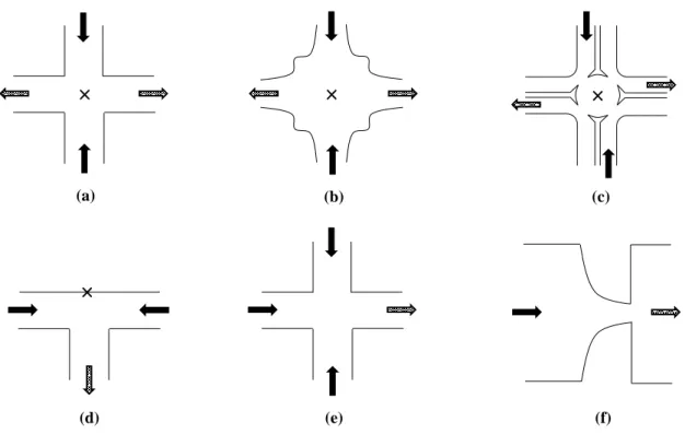
rheological properties of complex fluids in extension-dominated flows: (a) – standard cross-slot; (b) – optimized cross-slot (Alves, 2008); (c) – four-roll mill device (Lee et al., 2007); (d) – T-junction; (e) – flow-focusing device; (f) – contraction/expansion. In devices (a)-(d), the cross locates the stagnation point. ... 6 Figure 2.1 – Flowchart of the shape optimization routine. Words in italic identify the open-source

software that was used in the corresponding task. ... 13 Figure 2.2 – Schematic representation of the FFD base plane in its initial (non-optimized) configuration.

The location of each design point, p1 to p6, is represented by its distance from the origin (rn) and

the angle relative to the x-axis (θ). Points denoted as fp are fixed and delimitate the optimization region (the cross-sectional area of the channel is constant beyond those points). The dashed line is an axis of symmetry for the base plane. The inset scheme shows the dimensions of the FFD (w is the channel width and it is equal for the four arms), where the four dots represent fixed points (fp) in the main figure (points p1 to p5 are equally separated by the same angle; point p6 is at an angle

θ = 3π/2 rad). ... 14

Figure 2.3 – Schematic representation of the expansion base plane in its initial (non-optimized) configuration. The location of each design point, p1 to p5, is represented by its distance from the

origin (rn) and the angle relative to the x-axis (θ). Points denoted as fp are fixed and delimitate the

optimization region (the cross-sectional area of the channel is constant beyond those points). The dashed line is an axis of symmetry for the base plane. The inset scheme shows the dimensions of the expansion: both the optimized length (l) and the downstream channel width (wd) are expressed

as functions of the channel contraction width (wc). Points p1 to p5 are equally spaced by the same

(fixed) angle. ... 16 Figure 2.4 – Schematic representation of the two cost functions. If the points represent the sampled

velocity profile in a geometry, at a given iteration of the optimization cycle, then the residuals minimization cost function starts to fit a linear function to those points (red line) and minimizes the residuals of that fitting procedure (red arrows). On the other hand, the profile fitting cost function tries to minimize the distance of those points to a target profile represented by the black line (black arrows denote this distance). The first cost function only has effect inside the optimization length, while the other one also has influence outside this region. Only a restricted number of arrows (distances) was represented for illustrative purposes. ... 19 Figure 2.5 – DNA molecule represented by a bead-spring model (Nb = 11, Ns =10). ... 21

(11)

__________________________________________________________________________________

xi

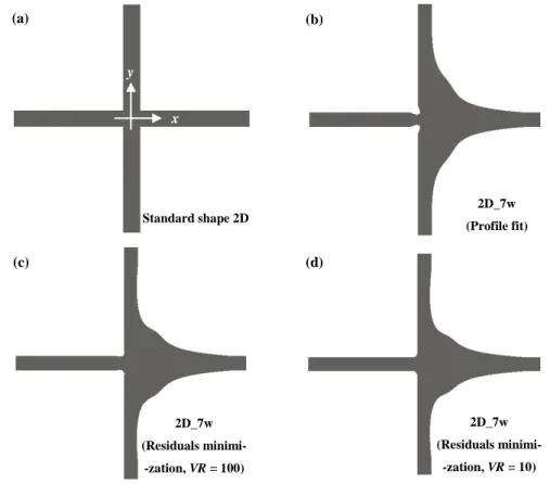
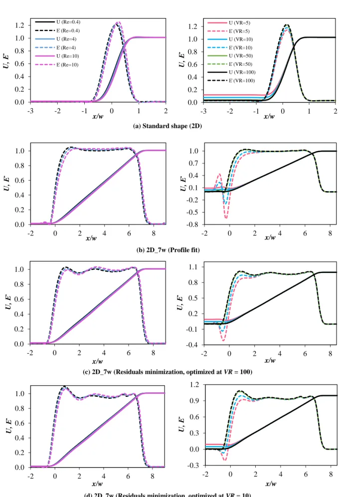
Figure 3.1 – Top view of the 2D standard and optimized geometries. Each arm of the FFD represented measures 8w from the origin (the Cartesian system illustrated in (a) is also valid for the other geometries). Figure (b) refers to the geometry optimized through a cost function that minimizes the deviation of the velocity profile at the centerline to an imposed profile (Eq. 2.4). Figures (c) and (d) represent the optimized geometries for a cost function that minimizes the residuals sum of the velocity profile fitted to a linear model (Eq. 2.3), at VR = 100 and 10, respectively. See Materials and methods section for references about the cost function and Table 2.1 for legend definition. ... 28 Figure 3.2 – Normalized velocity and deformation rate along the centerline of the FFD (y = 0) for

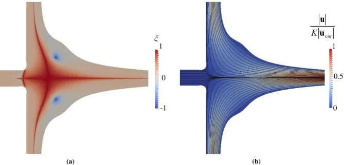
different flow conditions: in the left plots, VR = 100 and Re was the variable parameter; in the right plots, Re = 0.4 and VR was the variable parameter. The legend presented in (a) is also valid for the other plots. ... 29 Figure 3.3 – (a) Flow type parameter contour plot and (b) velocity map with superimposed streamlines

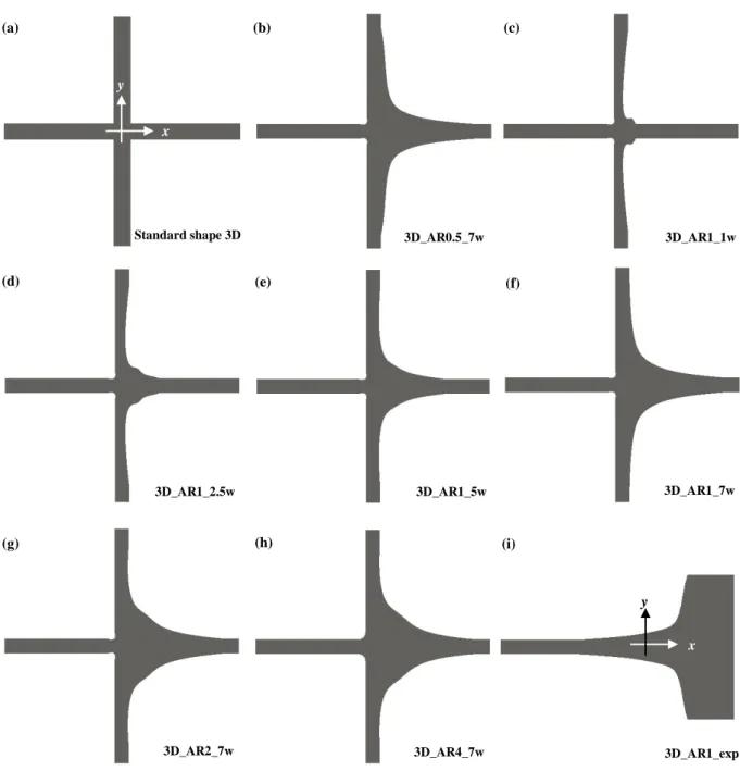
for the 2D_7w geometry (residuals minimization, optimized at VR = 100) at Re = 0.4 and VR = 100. ... 30 Figure 3.4 – Top view of the 3D standard and optimized geometries. Each arm of the FFD represented

measures 8w from the origin (the Cartesian system illustrated in (a) is also valid for geometries (b)-(h)). The expansion (i) is represented with a streamwise length of 15wc in the x-direction. See

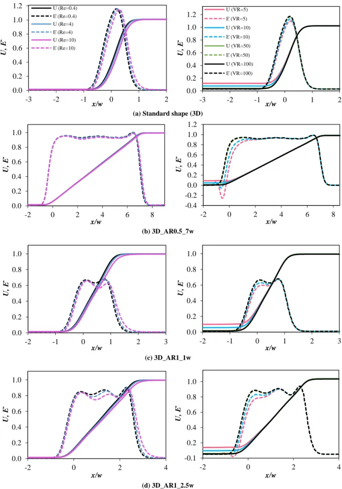
Table 2.1 for legend definition. ... 32 Figure 3.5 – Normalized velocity and deformation rate along the centerline of the FFD (y = 0, z = h/2)

for different flow conditions: in the left plots, VR = 100 and Re was the variable parameter; in the right plots, Re = 0.4 and VR was the variable parameter. The legend presented in plots (a) is also valid for the other plots. ... 33 Figure 3.6 – Normalized velocity and deformation rate along the centerlines at y = 0 and different z

positions for three different aspect ratios (devices): (a) AR = 0.5, (b) AR =1 and (c) AR = 2. The legend presented in plot (a) is also valid for the other plots. ... 36 Figure 3.7 – Normalized velocity and deformation rate along the centerline, at VR = 100 and Re = 0.4

for the numerical and analytical solution at different aspect ratios: (a) AR = 0.5, (b) AR = 1 and (c)

AR = 2. The corresponding shapes are depicted next to the profiles (black line – numerical solution;

blue line – analytical solution). The legend presented in (a) is also valid for the other plots. ... 38 Figure 3.8 – Experimental (points) and predicted (continuous lines) dimensionless velocity along the

centerline in three different geometries: (a) 3D_AR1_5w, (b) 3D_AR1_7w and (c) 3D_AR1_exp. ... 39 Figure 3.9 – (a) Dimensionless velocity and (b) first normal stress difference profiles, at the centerline

of the optimized FFD (2D_7w geometry, optimized at VR = 100 through the residuals minimization), for different We (Oldroyd-B, VR = 100, Re = 0.18, β = 8/9). The high frequency

(12)

__________________________________________________________________________________

xii

oscillations in the first normal stress difference profiles are due to the poor mesh quality at the centerline when the whole geometry is meshed. ... 40 Figure 3.10 – Streamlines in the 2D optimized FFD device (2D_7w geometry, optimized at VR = 100

through the residuals minimization) at different We (Oldroyd-B, VR = 100, Re = 0.18, β = 8/9). A steady symmetry breaking flow instability is observed in cases (c) and (d). ... 42

Figure 3.11 – Accumulated strain 

      



  w x s xx s t w x / 5 . 8 ) ( ) / ( 

  and travelling time of a molecule

advected along the centerline of the device (double 3D_AR1_7w geometry, VR = 100, We = 50). Both profiles were numerically computed... 43 Figure 3.12 – Average fractional length of λ-DNA computed in the double 3D_AR1_7w geometry for

two different velocity ratios/Hencky strains: (a) VR = 100 and (b) VR = 10. Note that the two symmetric FFD are linked by a straight channel located between x/w = -0.5 and x/w = 0.5 (this was required to allow the flow to develop in the transition region, in order to have a symmetric velocity profile with relation to x/w = 0). Three regions may be identified based on the molecular length evolution: region A (-8.5 < x/w < -0.5), region B (-0.5 < x/w < 7) and region C (7 < x/w < 8.5). See an example of individual results in Figure A.7. ... 44 Figure 3.13 – Fractional length as a function of the accumulated strain in the double 3D_AR1_7w

geometry, at VR = 100, predicted using different models (see the explanation in the text). The arrows point the evolution of the strain, which is related with the region in the double FFD (see the corresponding region, identified by letters, in Figure 3.12). The transition between regions A and B occurs at ε ≈ 5.3. The affine deformation curve was shifted vertically in the transition between regions A and B in order to match the fractional length predicted by the Brownian model at the exit of the free relaxation region, which facilitates the slope comparison (this was necessary because the affine deformation equation is not able to correctly predict the free relaxation). ... 46 Figure 3.14 – DNA maximum averaged fractional length in the double 3D_AR1_7w geometry as a

function of We, at different VR. The values were probed at the exit of the contraction region (x/w = -0.5), where the molecular elongation is maximum. The dotted line represents the stretch for an

infinite Hencky strain (50 strain units), according to the simple dumbbell model (Eq. 3.1). The

symbols represent the We at which simulations were performed (the connecting lines are only a guide to the eye). The inset is a zoomed view of the main plot at low We... 48 Figure 3.15 – Histogram of the fractional length at the exit of the contraction region of the double

3D_AR1_7w geometry (x/w = -0.5, as pointed out by the arrows in the scheme) for different We, at VR = 100. The arrows mark the averaged value, based on the simulation of 300 individual λ-DNA molecules. ... 49 Figure 3.16 – Average fractional length in the optimized double 3D_AR1_7w FFD and in a standard

(13)

__________________________________________________________________________________

xiii

Figure A.1 – Typical mesh used in the optimization routine (2D detailed view of the optimized geometry 3D_AR1_7w). ... 61 Figure A.2 – Relaxation curve of λ-DNA. The continuous line represents the exponential equation fitted to simulation data (points): <L2(t)> = 1.942_{+ 110exp(-t/4.2). Only points in the region L(t) < 6.3}

μm (0.3Lc) were considered in the fitting. ... 61

Figure A.3 – Effect of the dimension of the sampled population in the average fractional length of λ-DNA (double 3D_AR1_7w geometry, We = 50, VR = 100). ... 62 Figure A.4 – Normalized velocity and deformation rate along the centerline of the FFD (y = 0, z = h/2) for Re = 50 and VR = 100: (a) 2D geometries (PF – profile fit solution; RM – residuals minimization solution, optimized at VR = 100), (b) 3D geometries (l = 7w in all cases, only the aspect ratio changes). ... 62 Figure A.5 – (a) Normalized velocity and deformation rate along the centerline of the FFD (y = 0, z =

h/2) at Re = 0.4 for different VR and (b) corresponding streamlines at VR = 2400 (2D_7w geometry

optimized at VR = 100 through the residuals minimization). ... 62 Figure A.6 – Contour plot of the normalized first normal stress difference in the 2D_7w optimized FFD, at Re = 0.18, VR = 100 and We =1.7 for the Oldroyd-B model with β = 8/9. ... 63 Figure A.7 – Individual (black lines) and averaged fractional length (blue line) of λ-DNA (double 3D_AR1_7w geometry, We = 150, VR = 100). ... 63 Figure A.8 – Molecular configurations of λ-DNA when the simulation starts from a folded initial configuration (double 3D_AR1_7w geometry, We = 50, VR = 100). Note that the five molecular conformations illustrated are not drawn to scale with respect to each other. ... 64 Figure A.9 – Molecular configurations of λ-DNA when the simulation starts from a dumbbell-prone initial configuration (double 3D_AR1_7w geometry, We = 50, VR = 100). Note that the five molecular conformations illustrated are not drawn to scale with respect to each other. ... 65 Figure A.10 – Evolution of the fractional length of a λ-DNA molecule in a starting folded configuration being visible three intermediate plateaus that correspond to the unfolding process (double 3D_AR1_7w geometry, We = 50, VR = 100). The inset shows the molecule conformation in its folded state. ... 66 Figure A.11 – Orientation inversion and stretching in the y-direction (double 3D_AR1_7w geometry,

We = 50, VR = 100). The position in the device to which the zoomed view refers is identified in

the top-left inset. ... 66 Figure A.12 – Top view of the standard double FFD used in Brownian dynamics simulations (for comparison purposes) and flow streamlines computed in OpenFOAM. The blue dashed line is located at x/w = -2 and represents the departure position of molecules. All the arms of the device have the same width, which was made equal to the value used in the optimized FFD. ... 67

(14)

__________________________________________________________________________________

xiv

List of tables

Table 2.1 – Geometric parameters of the optimized devices (the geometry identifier is used in order to facilitate the identification of a given device; w – FFD channel width; wc – contraction width in

the expansion device). The aspect ratio for the 2D device is not presented since this was not relevant for the flow solver. ... 15

(15)

__________________________________________________________________________________

xv

List of symbols and abbreviations

Symbol SI Unit Description

A m2 Parameter of the exponential fit

b m.s-1 y-intercept of the linear regression

C – Constraints

fcost m2.s-2 Cost function

h m Channel height

K – Centerline to average velocity ratio

kB m2.kg.s-2.K-1 Boltzmann constant

l m Optimized region length

L m Molecule length

L0 m Molecule length at equilibrium

LC m Contour length

LS m Maximum extension of a spring

m s-1 Slope of the linear regression

Nb – Number of beads

Ns – Number of springs

p Pa Pressure

Q m3_.s-1 _{Flow rate}

r m Design point radius

rb m Bead radius

T K Absolute temperature

t s Time

U – Normalized velocity

v m3 Excluded volume potential parameter

w m FFD channel width

wc m Channel contraction width

wd m Channel width downstream of the contraction

wu m Channel width upstream of the contraction

(16)

__________________________________________________________________________________

xvi Greek symbols:

β – Solvent viscosity ratio

ε – Hencky/accumulated strain

ɛ̇ s-1 _{Deformation rate}

Ε̇ – Normalized deformation rate

ζ kg.s-1 Drag coefficient

θ rad Design point angle

λp m Persistence length

μ Pa.s Dynamic shear viscosity

μe Pa.s Extensional viscosity

μp Pa.s Polymer viscosity

μs Pa.s Solvent viscosity

ξ – Flow type parameter

ρ kg.m-3 _{Fluid density}

τ s Relaxation time

χ m Upper bound for design parameters

ψ m Lower bound for design parameters

Vectors and tensors:

D s-1 Deformation rate tensor

FB N Brownian force

FD N Drag force

FEV N Excluded volume force

FHI N Hydrodynamic force

fijS N Spring force between beads i and j

FS N Total spring force on a bead

S – Random vector

u m.s-1 Velocity vector

X m Inter-bead connection vector

x m Spatial position vector

σ Pa Extra-stress tensor

(17)

__________________________________________________________________________________

xvii Dimensionless groups:

AR – Channel aspect ratio

De – Deborah number El – Elasticity number Re – Reynolds number VR – Velocity ratio We – Weissenberg number Abbreviations Definition

CaBER Capillary Breakup Extensional Rheometer DLA Direct Linear Analysis

DNA Deoxyribonucleic acid FFD Flow-Focusing Device(s)

FiSER Filament Stretching Extensional Rheometer MADS Mesh Adaptive Direct Search

NOMAD Nonlinear Optimization by Mesh Adaptive Direct Search (software) PDMS Polydimethylsiloxane

PIV Particle Image Velocimetry

(18)

___________________________________________________________________________

Introduction | 1

1 – Introduction

1.1 – Motivation and thesis outline

In the last years, microfluidics has attracted the attention of the scientific community from many diversified fields. Furthermore, this area of research has successfully evolved from academia to the industry, which is confirmed by the increasing number of commercial microfluidic-based applications and devices. Several factors contributed to this interest, among which the small volume of fluids required and the particular behavior (inertial, diffusive, elastic, …) of the flow at the micro-scale. Although not being an immature science front, microfluidics still faces many challenges, both at the experimental and theoretical levels. One important challenge is the increase of the effectiveness and efficiency of microfluidic devices by optimizing its design.

This work presents an optimization procedure applied to a standard microfluidic device aiming to produce a homogeneous extensional flow in an wide region, which finds applications in rheological studies, molecular stretching (at single-molecule level), cell mechanics studies, droplet deformation, among others. In addition to the design strategy, an application of the optimized device is also presented, as well the experimental confirmation of the simulation results.

In the remainder of the “Introduction” section, several microfluidic geometries that create an extensional flow are reviewed in the context of a specific application. This is followed by the description of some design optimization cases that were successfully applied to microfluidic devices. The section ends with the formulation of the problem addressed in this work.

The “Materials and Methods” section describes the set of computational and experimental techniques that were adopted in order to optimize and test the microfluidic device. The results that were obtained are presented in the “Results and discussion” section. Lastly, a brief conclusion is presented, which summarizes relevant results and the suggestions for further work.

1.2 – Microfluidic devices for extensional flow

In fluid mechanics there are two essential and opposite types of flows, from a rheological perspective: rotational and extensional flows. In between these two extremes, there are shear flows, Figure 1.1, which are also very important in rheometry.

(19)

___________________________________________________________________________

Introduction | 2 Figure 1.1 – 2D element of fluid in different types of flow (solid lines – initial form; dashed lines – final form).

The different types of flow arise as a consequence of velocity gradients. Indeed, an extensional flow exists when there is a velocity gradient in the direction of the flow, while shear flows occur when there is a velocity gradient normal to the flow direction, such as in a steady pipe flow, where the velocity gradient is primarily due to the fluid viscosity. In order to identify which type of flow is predominant in a given situation, the dimensionless flow-type parameter,

ξ, can be used (Lee et al., 2007):

Ω D Ω D     (1.1) where



 

T



2 1 u u

D    is the deformation rate tensor (u is the velocity vector) and

 



T



2 1 u u

Ω    is the vorticity tensor. A rotational flow is characterized by ξ = -1 (no extensional deformation, |D| = 0), while an extensional flow corresponds to ξ = +1 (no rotation, hence D is a traceless diagonal tensor).

The focus of the present work is on extension-dominated flows. This type of flow assumes a recognized importance when polymers and/or microscopic entities like cells are present. In joints, the synovial fluid (with a high concentration of hyaluronic acid) is compressed between both bones of the articulation in an extensional-like flow (Haward et al., 2013a). The blood circulation also has an important extensional component, for instance in stenosis structures (Tovar-Lopez et al., 2010). Moving to a completely different field, extensional flow plays a key role in jet pointers, which is reflected on the printing quality (Hoath

et al., 2014). In addition, different microfluidic devices were specifically designed in order to

produce extensional flows, with several purposes. Among them, three groups are distinguished and discussed in the following sections: devices for rheological studies, devices for molecular stretching and devices for the deformation of biological cells. Note that these groups are not mutually exclusive, since the same device may be suitable for multiple purposes.

Extensional flow Shear flow

(20)

___________________________________________________________________________

Introduction | 3 1.2.1 – Rheological studies

The extensional viscosity is complementary to the shear viscosity when characterizing a material. However, the extensional viscosity is significantly more difficult to measure than shear viscosity. Some reasons may be pointed that support this fact: (1) difficulty in the generation of purely extensional flows; (2) dependence of the extensional viscosity on both strain rate and accumulated strain; (3) the low relaxation times (< 1 ms) of some dilute solutions requires an extremely high strain rate to be applied in order to effectively stretch the molecules (We = τɛ̇ > 0.5, where We is the Weissenberg number, τ is the relaxation time of the fluid and ɛ̇ the deformation rate), which usually increases inertial effects (Haward & McKinley, 2013b). Given these difficulties, microfluidic devices arise as a very promising solution for extensional rheometry.

Microfluidic devices that impose an extensional flow have been widely used in the rheological study of complex (non-Newtonian, namely viscoelastic) fluids. Such devices take the advantage of a high Elasticity number (El = De/Re, where De is the Deborah number and

Re is the Reynolds number), which enhances the elastic behavior, while keeping a low Reynolds

number flow, which minimizes inertial effects. Thus, fluids with a low viscosity and relaxation time may be characterized in these devices, which would be challenging in macroscale rheometers like the CaBERTM (Capillary Breakup Extensional Rheometer) or FiSERTM (Filament Stretching Extensional Rheometer) devices. Although the comparison between rheometers at different scales is out the scope of this work, it should be noted that devices like the CaBERTM and FiSERTM are able to produce an uniaxial extension with low shear due to the absence of solid surfaces in contact with fluid (the free surface may be, however, a source of instability, Minoshima & White, 1986), while the extension in microfluidic devices is planar (with few exceptions) and the wall shear cannot be neglected in most cases.

From a rheological perspective, two aspects may be accessed in extensional flows: the extensional viscosity (and its dependence on the deformation rate, ɛ̇, and on the Hencky strain,

ε = ɛ̇t) and development of (inertio-)elastic instabilities. Some illustrative examples are briefly reviewed in the following paragraphs. It should be noted that these studies on extensional flows are used not only for experimental purposes, but also to test (verify) the predictive capacity of computational fluid models (see for instance, Schoonen et al., 1998).

Stagnation-point microfluidic devices were successfully used for the measurement of the extensional viscosity and in the study of flow instabilities. The cross-slot device, composed of two opposite incoming streams with two laterally opposed outlets normal to the inlet

(21)

___________________________________________________________________________

Introduction | 4 channels, Figure 1.2(a), is able to retain molecules at its stagnation point (with zero velocity, but finite and non-zero strain rate, controlled by the flow rate) for a long time. This feature allows molecules to accumulate a high Hencky strain, which is linearly proportional to the time they remain at the stagnation point. Auhl et al. (2011) expressly took advantage of the high accumulated strain to evaluate the steady-state extensional behavior of polymer melts and to test the predictive capability of material models. However, a major drawback of this device is the reduced area where the strain rate is constant, which is nearly limited to one channel width (see for instance, Haward et al., 2012a). In order to circumvent this limitation, Alves (2008) used a numerical optimization procedure that increased the constant strain rate region to 7.5 channel widths, either side of the stagnation point, in a 2D cross-slot, Figure 1.2(b). More recently, the same process was extended to a 3D configuration of the cross-slot (Galindo-Rosales et al., 2014). Haward et al. (2012b) tested the 2D shape-optimized cross-slot as an extensional rheometer for dilute polyethylene oxide solutions for deformation rates in the range 26–435 s-1. Both the measurements of birefringence and pressure drop were self-consistent and in good agreement with theoretical models. The same optimized cross-slot was also used to investigate elastic instabilities, which are important to determine the operational limits of the device (Haward & McKinley, 2013b). Two major advantages of the optimized device are the wide region available to measurements and the reduction of the shear stress in the vicinity of the centerline due to a lubricating film of fluid in the corners of the device and to the increased distance of corners to the stagnation point. The standard (perpendicular channels) cross-slot was also used in the study of elastic instabilities of wormlike micellar solutions (Dubash et al., 2012; Haward et al., 2012a) and other complex fluids (Puangkird et al., 2009; Rocha et al., 2009; Schoonen et al., 1998), both using experimental and computational approaches. The shape of this device is particularly suitable to the study of elastic instabilities due to the flow curvature around its corners and to the large normal stress difference that is developed. Other stagnation-point devices exist, as the four-roll mill device, Figure 1.2(c), and T-junctions (a bifurcating channel), Figure 1.2(d). The four-roll mill device has the notable capacity to alternate between rotational, shear and extensional flows, through the simple control of the flow rates through its four inlets and four outlets, in the microfluidic configuration proposed by Lee

et al. (2007).

Flow-focusing devices (FFD) have received less attention than cross-slot for rheological studies. These devices are similar to a cross-slot in the number and configuration of channels. However, while in the cross-slot there are two inlets and two outlet streams, in a

(22)

___________________________________________________________________________

Introduction | 5 FFD there are three inlets and one outlet stream, Figure 1.2(e). This allows the compression and alignment of one stream due to the squeezing effect of the other two. Unlike in cross-slot devices, there is no stagnation point in a FFD and, consequently, the Hencky strain has a limited value, which depends on the flow rate ratio between the side and central streams (ε = ln(2VR + 1) for a FFD whose arms have the same width; VR is the side-to-central velocity ratio). Thus, steady-state elongation will only conditionally occur. Arratia et al. (2008) used a FFD to estimate the extensional viscosity of a dilute polymer solution based on the thinning of a (2D) filament. This method takes the advantage of reduced shear due to the lubricating effect of lateral streams, since two immiscible fluids were used in experiments, although the extensional region is still restricted to about one channel width. Oliveira et al. (2009) computationally studied the development of purely elastic instabilities in a FFD. To the best knowledge of the author, no optimization procedure was explicitly applied on this device in order to increase its performance for rheological studies. The major shape modifications performed on this geometry were made in the context of droplet generation, a field where FFD are widely used (Chae et al., 2009; Roberts et al., 2012; Teh et al., 2008).

The last class of microfluidic devices reviewed in this section includes contraction /expansion microchannels. As depicted in Figure 1.2(f), these devices comprise a straight channel with a contraction that is responsible for the fluid acceleration in the flow direction. This contraction can assume several shapes and it may be followed by an abrupt or smooth expansion (which may be linked through a straight channel region, as in Oliveira et al., 2008). The extensional deformation profile depends both on the flow rate and on the contraction shape (Sousa et al., 2011). The accumulated (Hencky) strain is related with the aperture of the contraction relative to the upstream channel width: ε = ln(wu/wc), where wu is the upstream channel width and wc is the contraction width. Hyperbolic contractions were specifically designed (based on the simple proposition that if the contraction cross-sectional area decreases inversely proportional to the axial position, then the extension rate will be constant, Ober et al., 2013, although some deviation was observed due to shear effects at the walls) to achieve a constant strain rate profile (Campo-Deaño et al., 2011; Ober et al., 2013). Such hyperbolic contractions were reasonably accurate as extensional rheometers up to extensional rates of 103

s-1_{, when combined with optical (birefringence) and pressure drop measurements (Ober et al.,}

2013). However, the imposition of a high Hencky strain requires a large difference between the contraction and upstream channel widths, which may be problematic for standard PDMS (polydimethylsiloxane) devices (in Ober et al., 2013 the Hencky strain was only ɛ = 2, for a

(23)

___________________________________________________________________________

Introduction | 6 width ratio of 7.4). A slightly different application for hyperbolic contractions was found by Campo-Deaño et al. (2011), allowing to the measurement of the relaxation time of Boger fluids based on the self-similar vortex growth upstream the contraction for different viscoelastic fluids. Sousa et al. (2011) have demonstrated the importance of extensional rheology of blood analogues, validating their flow through differently shaped microcontractions. As in cross-slot and FFD, elastic instabilities were also analyzed in contraction/expansion devices (Oliveira et

al., 2008).

Figure 1.2 – Schematic representation (top view) of microfluidic devices applied in the study of rheological

properties of complex fluids in extension-dominated flows: (a) – standard cross-slot; (b) – optimized cross-slot (Alves, 2008); (c) – four-roll mill device (Lee et al., 2007); (d) – T-junction; (e) – flow-focusing device; (f) – contraction/expansion. In devices (a)-(d), the cross locates the stagnation point.

Based on the previous discussion on microfluidic devices suitable for rheological studies in extension-dominated flows, some relevant characteristics of such an idealized device are identified: (1) produce a homogeneous extensional flow (shear-free), which should be Re (inertia) independent; (2) keep the deformation rate constant over an extended region, suitable for measurements using optical techniques; (3) able to analyze fluids in a wide range of viscosities and relaxation times (mostly critical for low viscosity fluids); (4) easily control the deformation rate and Hencky strain; (5) easy fabrication and operation, at a low-cost.

The reader interested on extensional micro-rheometers is directed to recent reviews on this subject (Galindo-Rosales et al., 2013; Pipe & McKinley, 2009).

(a) (b) (c)

(24)

___________________________________________________________________________

Introduction | 7 1.2.2 – Stretching of macromolecules (single-molecule level)

The molecular stretching performed by extensional flows finds several applications other than pure rheological studies, which are briefly discussed in this section. Without surprise, microfluidic devices employed in these types of applications are very similar to those discussed previously.

Chan et al. (2004) proposed the DLA (Direct Linear Analysis) method to rapidly accomplish the mapping of DNA (Deoxyribonucleic acid) molecules. This technology, actually traded by PathoGenetixTM, is based on DNA labeling by fluorescent markers, which bind to specific sites of the molecule where a given base pair sequence exists. The result is a barcode like pattern that is specie-dependent and that allows (fast) microbial genotyping without nucleotide sequencing. In order to guarantee the method reproducibility, DNA molecules must be probed in a stretched state (Chan et al., 2004). This task was accomplished, in the original configuration (Chan et al., 2004), by an array of obstacles followed by a microfluidic contraction to impose an extensional and confined (1 μm deep channels) flow that unraveled DNA molecules. A subsequent study was published by the same group where several configurations were tested for the microcontraction (Larson et al., 2006). The geometries which imposed a constant deformation rate and linear increasing deformation rate gave the best results, since they were able to deliver a DNA population in a highly stretched state (averaged extension up to 87 % of λ-DNA contour length, although for De > 50), with a relatively low dispersion in the length distribution function. The DNA stretching device was further modified by the same group to a microcontraction followed by a FFD fused with another microcontraction (Krogmeier et al., 2007). It should be noted that in applications such as DLA and general sequencing techniques, the throughput of the method is of high concern.

A DLA-related DNA mapping was investigated by Dylla-Spears et al. (2009). In this method, a standard cross-slot device is used to trap DNA molecules previously mixed with sequence-specific markers. The molecular extension has shown to be a critical factor in the accuracy and resolution of the method, since the markers position (and inter-markers distance) is not fixed between different assays unless DNA molecules keep their full extension. In this way, the cross-slot device is even more suitable than the microcontraction in DLA, since it potentially allows a steady stretched state due to its stagnation point. Indeed, the method resolution was higher than that reported in DLA and the same degree of extension was achieved at a lower De (88 % of λ-DNA contour length, at De = 3.9) (Dylla-Spears et al., 2009). However, the stagnation point also represents a throughput decrease.

(25)

___________________________________________________________________________

Introduction | 8 The theoretical background in the design of techniques for molecular stretching, as in the two cited examples, is primarily based on single-molecule studies. Such studies aim to explore the molecular behavior in diversified flow conditions. Extensional flows are of great importance for this purpose. Cross-slot devices (Hsieh et al., 2007; Perkins et al., 1997; Schroeder et al., 2003; Smith & Chu, 1998), FFD (Wong et al., 2003), T-junctions (Tang & Doyle, 2007) and contraction/expansion devices (Chuncheng & Qianqian, 2009; Hsieh et al., 2011; Huang et al., 2014; Randall et al., 2006) were used both in experimental and theoretical studies. It should be noted that, due to the electric charge of DNA molecules, the motion force may be provided by an electrical field, as well by an imposed pressure gradient. The former has proved to be especially advantageous over the second owing to the symmetry of the velocity gradient (hence, with irrotational components even near the walls) and to the quadratic decay of field disturbances (Randall & Doyle, 2005).

A note about DNA stretching techniques should be made at this point. There are several other methods, in addition to extensional flow devices, to stretch individual molecules: optical tweezers (Wang et al., 1997), flow past an array of obstacles (Teclemariam et al., 2007), oscillatory flow fields (Jo et al., 2009), flow past tethered DNA (Ferree & Blanch, 2003), thermo-electrophoresis (Hsieh et al., 2013) and functionalized surfaces (Liu et al., 2014). However, throughput, among other aspects, is generally an issue in these methods, although this obviously will depend on the specific application.

As in the previous section, the discussion about microfluidic devices that aim to stretch DNA in extensional flows ends with the idealized characteristics of such a device intended to deliver stretched DNA to a downstream analytical process. The characteristics are the same as those mentioned in the previous section, to which it should be added the ability to achieve high throughputs. Note that, while for rheological studies it is important to generate pure extensional flows, for DNA stretching this condition is not so strict. The only requirement is the delivery of a homogeneously stretched population of DNA molecules to ensure the reproducibility of the analytical procedure that follows the stretching event. However, since the presence of shear forces may increase the dispersion of stretched states (Larson et al., 2006), then homogeneous extensional flows are also desirable in such applications.

1.2.3 – Other applications

Extensional flows are also of interest in the study of mechanical properties of biological cells. Yaginuma et al. (2013) assessed the rigidity of red blood cells in a hyperbolic

(26)

___________________________________________________________________________

Introduction | 9 contraction device, highlighting its potential for diagnosis purposes. Also inspired on cell deformability, Gosset et al. (2012) proposed a mechanical phenotyping technique that includes a stagnation point geometry. More precisely, biological cells are focused and directed to a cross-slot device, where they are imaged in a stretched state. This technique proved to be able to distinguish between healthy and cancerous cells based on the differences of extensibility.

1.3 –Optimization of microfluidic devices

An optimization problem may be conceptually formulated as a problem where the objective is to find the set of parameters r = {r1, …, rn}, eventually delimited between a lower

ψ = { ψ1, …, ψn} and upper bound χ = { χ1, …, χn} – box constraints –, that minimizes, global or locally, a cost function fcost(r1, …, rn), subjected to a set of linear/non-linear C(r) constraints:



1,..., n

 

1,..., n

 

1,..., n



, ... : ) ) ,..., min(f_cost(r₁ r_n C₁(r)k₁  C_m(r)k_m    r r    (1.2) There are several algorithms that could be used to find the optimal solution of the

problem and it is common to distinguish between gradient-based methods and free-derivative methods. Gradient-based methods rely on the direct computation (analytical or numerically) of the derivative (first and/or higher order) of the cost function, since it is well known that the derivative of a function at a minimum is zero (applied, for instance, in Newton’s method) and, also, that the derivative/gradient of a function points to the direction of maximal change (applied, for instance, in the gradient descent method). However, the cost function is not always continuously differentiable and computing its derivative could be expensive, complex or inaccurate (due to noise) in real engineering problems. Free-derivative algorithms arise as a robust alternative for these situations, though at the cost of a slower convergence to the optimal solution.

Rios & Sahinidis (2013) further classified free-derivative algorithms with respect to three criteria: direct vs. model-based; local vs. global; stochastic vs. deterministic. Direct methods perform a sampling procedure of the cost function at a given set of points, which are updated in the next iteration after defining the searching direction and the step length. On the other side, model-based methods evaluate the cost function in order to adjust a simple, but accurate model (usually a second-order polynomial) to the cost function. This allows the computation of the searching direction from the model. The difference between local and global methods is based on its capacity to escape local minima and the classification of a method as deterministic or stochastic depends on the respective randomness. In brief, these methods differ in the way they use the current set of design parameters to generate the next guess and it is not

(27)

___________________________________________________________________________

Introduction | 10 possible to point the best algorithm, since it will always depend on the specific problem. The reader interested on free-derivative optimization algorithms, as well on their implementation on available software and relative performance, is directed to Kramer et al. (2011), Moré & Wild (2009) and Rios & Sahinidis (2013).

From a practical perspective, optimization routines are of common practice in fluid and solid dynamics processes. A classical and well-known problem is the drag reduction of vehicles through shape modifications, as an attempt to decrease the fuel consumption (Muyl et

al., 2004; Song et al., 2012). Of particular importance for the present work is the optimization

of microfluidic devices and illustrative examples of such cases are presented in what follows. Mixing two or more fluids at the micro-scale is a great challenge, since low Re flows avoid turbulence effects that promote the mixing of fluids. Shuttleworth et al. (2011) addressed this problem through the shape optimization of a set of electrically conductive posts in an induced charge electro-osmosis process. The asymmetric vortex structures that arise near posts, due to the charge balance in the respective double layer, increase the interfacial area between fluids. Thus, a good inter-dispersion of fluids was achieved without diluting the mixture, since the device can operate as a static mixer, with a constant volume of fluid. The optimization routine was performed with a parallel free-derivative direct local search algorithm that directly sampled the cost function (level of heterogeneity in the mixture concentration) according to a direction and step length, as explained previously for direct methods. In this case, the design parameters controlled both the shape and location of posts.

The work of Ivorra et al. (2006) was related with the same mixing phenomena. More specifically, the authors aimed to minimize the mixing time of a protein solution in a FFD, since this is crucial in the study of fast folding events that occur with these biomolecules. The objective – minimization of the mixing time – was accomplished through the parameterization of the FFD corners (shape optimization). Two algorithms were tested by the authors, namely a stochastic genetic algorithm and a semi-deterministic algorithm, where the gradient of the cost function was computed based on the physical equations. The mixing time was successfully decreased to less than 50 % of its initial value.

In section 1.2.1, a reference was made to an optimized cross-slot device designed by Alves (2008), Figure 1.2(b), which has a wider region of constant deformation rate. The optimization was also performed at the parameterized corner of the device and a free-derivative local model-based search algorithm was employed to find a minimum of the cost function.

(28)

___________________________________________________________________________

Introduction | 11 A different approach was presented by Jensen et al. (2012) who designed a microfluidic viscoelastic rectifier using topological optimization. This method attributes to each cell in the computational domain a coefficient that represents a virtual porosity. Depending on the porosity value, a cell may behave as a void, with fluid flow, or as a solid, with nearly no-slip conditions. The porosity coefficient is incorporated in the Navier-Stokes equations and a posterior sensitivity analysis (gradient-based) identifies the contribution of each cell to the minimization of the cost function. As a result, the optimization is applied on the whole computational domain, so that the number of design variables depends on the level of discretization of the initial geometry, in the region to be optimized.

1.4 – Problem formulation

At this point, it is clear that the same microfluidic device may be suitable for several applications, although there is not a device that performs ideally in all applications. Flow-focusing devices are particularly interesting from this perspective. Indeed, these devices meet almost all the idealized characteristics enumerated for the two applications previously described. Furthermore, the throughput is higher than in stagnation point devices (although at the cost of a lower Hencky strain) and higher Hencky strains are more easily reached/controlled than in contraction/expansion devices. Still, a major drawback of standard FFD is their limited region of extensional flow, which is not perfectly homogeneous.

In order to solve this problem, a design optimization can be used. This task could be accomplished based on the same approach as in Ober et al. (2013) applied to a contraction/expansion geometry (see section 1.2.1). Nevertheless, entry effects are important when the geometry becomes abrupt and this reason may explain the non-ideal behavior observed by Ober et al. (2013). A more robust approach would be a numerical shape optimization, as in Alves (2008), and this was in fact the strategy adopted for this work. Topological optimization would also be a valid alternative and it is left as a suggestion for a future work. For the solution of this problem, another challenge was set: to use only open-source software. Although this was not a major goal, it demonstrates that the type of approach here presented is free of costs in what concerns software licensing.

In the next section, the strategy adopted is explained, as well as the experimental procedure to validate the simulated results of the final optimized shape. Additionally, Brownian dynamics simulations were performed to evaluate the potential of the optimized devices in the extension of DNA molecules and the model employed is also described in the next section.

(29)

___________________________________________________________________________

Introduction | 12 Before proceeding further, a citation of Binding & Walters (1988) is here reproduced about the task of designing devices for pure extensional flows: “Generating a purely extensional flow in the case of mobile liquids is virtually impossible. The most that one can hope to do is to generate flows with a high extensional component and to interpret the data in a way which (hopefully) captures that extensional component in a convenient and consistent way through a suitably defined extensional viscosity and strain rate. The philosophy is not without its difficulties and is somewhat controversial. However, given the practical importance of the subject and the expectation that there will be at least semi-quantitative predictive capacity, it is our contention that the pursuit is eminently worthwhile, especially since there is no alternative if one requires some indication of the extensional viscosity levels in the flow of non-Newtonian elastic liquids”.

(30)

___________________________________________________________________________

Materials and methods | 13

2 – Materials and methods

2.1 – Shape optimization routine

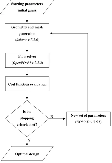
Figure 2.1 presents a schematic representation of the general procedure that was implemented to optimize the FFD.

Figure 2.1 – Flowchart of the shape optimization routine. Words in italic identify the open-source software that

was used in the corresponding task.

Briefly, the standard, non-optimized FFD, was parameterized on its corners and meshed on Salome-platform v.7.2.0 (Ribes & Caremoli, 2007). This was fed as input to OpenFOAM v.2.2.2 (www.openfoam.org) which was used to compute the flow field. Next, the velocity was sampled at the centerline of the geometry and the cost function was computed.

Starting parameters (initial guess)

Geometry and mesh generation

(Salome v.7.2.0)

Flow solver

(OpenFOAM v.2.2.2)

Cost function evaluation

Is the stopping criteria met?

New set of parameters

(NOMAD v.3.6.1)

Optimal design Y

(31)

___________________________________________________________________________

Materials and methods | 14 The new set of parameters, for the next iteration, was determined by the optimization algorithm coded in NOMAD v.3.6.1 (Audet et al., 2009; Le Digabel, 2011) and the cycle was repeated until the established convergence criteria was met. Each step of the flowchart is described in detail below.

2.1.1 – Geometry/mesh generation

The standard FFD geometry was parameterized on its corners through two Bézier curves, as depicted in Figure 2.2.

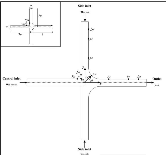
Figure 2.2 – Schematic representation of the FFD base plane in its initial (non-optimized) configuration. The

location of each design point, p1 to p6, is represented by its distance from the origin (rn) and the angle relative to the x-axis (θ). Points denoted as fp are fixed and delimitate the optimization region (the cross-sectional area of the channel is constant beyond those points). The dashed line is an axis of symmetry for the base plane. The inset scheme shows the dimensions of the FFD (w is the channel width and it is equal for the four arms), where the four dots represent fixed points (fp) in the main figure (points p1 to p5 are equally separated by the same angle; point p6 is at an angle θ = 3π/4 rad). w w 7w 7w l ½w ½w Central inlet uin, central Side inlet uin, side Side inlet -uin, side Outlet uout fp1 fp2 fp3 fp4 p6 p p2 p1 3 p4 p5 y x r3 θ

(32)

___________________________________________________________________________

Materials and methods | 15 Five points (p1 to p5) control the shape of the downstream corner, through their distance rn to the origin (θ angles were kept fixed), while only one parameter (r6) was allowed in the upstream corner. The upstream corner was only parameterized in order to obtain a rounded edge, since sharp edges are more prone to trigger instabilities in viscoelastic flows – the cost function was practically insensible to this parameter. Note that all the dimensions of the geometry are defined as a function of the channel width.

The FFD was optimized both in 2D and 3D configurations, since each one is more suitable for a given application. For instance, a 2D configuration is preferred for rheological studies because the high aspect ratio reduces wall effects in birefringence measurements. On the other side, 3D geometries are more amenable to be produced by PDMS micro-molding, which is a popular technique due to its low-cost and simplicity. Additionally, 3D configurations were optimized for four different values of the l parameter (length of the extensional region, Figure 2.2), at a fixed aspect ratio, where the aspect ratio is the height to width ratio: AR = h/w, and for four different values of AR, at a fixed optimized length (l). Those conditions are summarized in Table 2.1.

Table 2.1 – Geometric parameters of the optimized devices (the geometry identifier is used in order to facilitate

the identification of a given device; w – FFD channel width; wc – contraction width in the expansion device). The aspect ratio for the 2D device is not presented since this was not relevant for the flow solver.

Configuration Geometry identifier Aspect ratio (AR) Optimized region length (l) 2D 2D_7w - 7w 3D 3D_AR1_1w 1 1w 3D_AR1_2.5w 2.5w 3D_AR1_5w 5w 3D_AR0.5_7w 0.5 7w 3D_AR1_7w 1 3D_AR2_7w 2 3D_AR4_7w 4 3D_AR1_exp 1 7wc

Since the forced relaxation of highly stretched molecules may be also useful (and has received less attention than the extension), an expansion geometry was optimized for this purpose, Figure 2.3, which can be coupled at the outlet of a FFD. For this case, only one 3D configuration was optimized, at AR = 1, Table 2.1. Note that the final optimized shape could also be used as a contraction, in the same way the FFD may be used as an expansion by reversing the flow direction.

(33)

___________________________________________________________________________

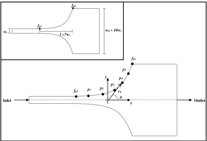
Materials and methods | 16 Figure 2.3 – Schematic representation of the expansion base plane in its initial (non-optimized) configuration. The

location of each design point, p1 to p5, is represented by its distance from the origin (rn) and the angle relative to the x-axis (θ). Points denoted as fp are fixed and delimitate the optimization region (the cross-sectional area of the channel is constant beyond those points). The dashed line is an axis of symmetry for the base plane. The inset scheme shows the dimensions of the expansion: both the optimized length (l) and the downstream channel width (wd) are expressed as functions of the channel contraction width (wc). Points p1 to p5 are equally spaced by the same (fixed) angle.

The Salome platform was selected as the geometry/mesh generator software, since it allows the construction of unstructured meshes. This type of meshes are more flexible than structured ones, although being also computationally more expansive. Note that in the present work, a new mesh was generated at each optimization iteration. Other authors only deformed a fixed mesh (Alves, 2008), although this procedure applied in the present work (on structured meshes) led to highly skew and heterogeneous meshes that compromised the convergence of the flow solver. Furthermore, the mesh generation was not the time limiting step in the optimization cycle.

In order to keep the mesh resolution constant, independently of the geometrical shape, the parameter that was specified in the mesh builder was the minimal/maximal cell size. Reference values of w/30 and w/20 for the minimal and maximal cell lengths (in all space dimensions, except in the z direction for the 2D dimensional case), respectively, were used,

y x θ fp2 fp1 p5 p4 p2 p1 p3 r4 Inlet Outlet fp2 fp1 wc wd = 10wc l =7wc

(34)

___________________________________________________________________________

Materials and methods | 17 based on a preliminary mesh independency study. The mixing of quadrangles with triangles was allowed, resulting in hexahedra-dominant meshes (Figure A.1).

2.1.2 – Flow solver

OpenFOAM, an open-source CFD software, was a straightforward choice to solve the flow field based on its applicability to viscoelastic fluids and high accuracy and stability. OpenFOAM is a finite volume C++ based CFD code that has a set of built-in solvers and also allows for the user to modify existing solvers or create its own solver. It offers several numerical schemes and, importantly, it handles unstructured meshes.

The built-in simpleFoam solver was directly used (after switching-off turbulence models) due to the flow characteristics: Newtonian and incompressible fluid, laminar and isothermal steady-state flow. This solver provides a solution for the steady-state Navier-Stokes equations: 0    u (2.1) u uu  2     p (2.2) Equation (2.1) represents the mass conservation (continuity equation), while (2.2) is the momentum conservation equation, where μ represents the fluid dynamic viscosity, ρ the fluid density and p the pressure. Field interpolations were performed through a standard central differencing scheme.

Boundary conditions were defined as follows. A fixed uniform velocity was assigned to all three inlets and a zero relative pressure was fixed at the outlet (while keeping a zero velocity gradient). To ensure the complete development of the flow at the entry to the optimized region and to avoid boundary perturbations at the outlet, both side channels and the outlet channel were extended 3 channel widths beyond the fixed points. In order to minimize inertial effects, Re at the outlet (here defined as Re = ρ|ūout|w/μ, where |ūout| is the average superficial

velocity at the outlet) was kept below 1 (typically, Re = 0.4). An important variable to consider in the FFD is the velocity ratio between inlet streams, here defined as VR = |uin, side|/|uin, central|.

Two different VR were tested in the optimization of the 2D_7w geometry: VR = 10 and 100. Note that while Re controls the total inflow (sides + central), it is the VR that determines the distribution of this flow between inlets (|ūout| = μRe/(ρw) = |uin, side| (2 + 1/VR)). The no-slip

condition was imposed on walls through a zero velocity on it and, in 2D geometries, the top and bottom planes were considered as empties. Due to the symmetry of the FFD on the Oxz plane, only half of the geometry was solved. In the case of the expansion geometry, Re is the