Acoustic estimation of seafloor parameters: A radial basis
functions approach
Andrea Caitia),b)
DIST, University of Genova, via Opera Pia 13, 16145 Genova, Italy Sergio M. Jesusc)
UCEH, University of Algarve, Campus de Gambelas, 8000 Faro, Portugal ~Received 20 October 1995; accepted for publication 22 May 1996!
A novel approach to the estimation of seafloor geoacoustic parameters from the measurement of the acoustic field in the water column is introduced. The approach is based on the idea of approximating the inverse function that links the geoacoustic parameters with the measured field through a series expansion of radial basis functions. In particular, Gaussian basis functions are used in order to ensure continuity and smoothness of the approximated inverse. The main advantage of the proposed approach relies on the fact that the series expansion can be computed off-line from simulated data as soon as the experimental configuration is known. Data inversion can then be performed in true real time as soon as the data are acquired. Simulation results are presented in order to show the advantages and limitations of the method. Finally, some inversion results from horizontal towed array data are reported, and are compared with independent estimates of geoacoustic bottom properties. © 1996 Acoustical Society of America.
PACS numbers: 43.30.Ma, 43.30.Pc@MBP#
INTRODUCTION
Geoacoustic seafloor properties are an essential requisite to properly predict acoustic propagation, especially in shal-low water wave guides and/or at shal-low frequencies. However, their measurement or estimation with traditional techniques requires the deployement of instrumentation on or within the seafloor ~such as geophone stations, coring, cone penetrom-eters, etc.!, resulting in costly and time-consuming proce-dures. For this reason, there has been a growing interest in recent years in methods able to identify geoacoustic models from the measurement of the acoustic field in the water col-umn. This approach, that can be regarded as acoustic remote sensing of the seafloor, is characterized by two major as-pects: one is experimental, and is concerned with the suitable design of sensors, sources, and at-sea procedures to accu-rately measure the acoustic field structure. The other is com-putational, and consists in the determination of a stable in-version algorithm able to uniquely recover the geoacoustic parameters from the measured field. This article is mainly concerned with the computational part of the estimation problem, i.e., with the inversion strategy.
Realistic attempts at geoacoustic characterization from the acoustic field were started by Frisk and co-workers.1–5 From the computational viewpoint, they mainly used a per-turbative inversion approach, i.e., a linearization of the in-verse problem in the neighborhood of an a priori known background geoacoustic model. If the background model is sufficiently close to the true model, powerful methods of linear inverse theory can be employed and the true solution can be found.3
The background model can sometimes be established using historical data or independent measurements. How-ever, when a confident background model cannot be estab-lished, the inverse problem is strongly nonlinear. In this more general case, the estimation of the geoacoustic param-eters is usually stated as an optimization problem and global search strategies have to be employed. Collins and co-workers have successfully shown how the simulated anneal-ing algorithm can be employed to estimate bottom parameters.6,7 Further applications of the simulated anneal-ing search have been reported by Dosso et al. and Chapman
et al.8,9
Another global search approach, the so-called genetic algorithms, was more recently introduced to the underwater acoustic community by Gerstoft.10Applications of this inver-sion strategy to field data have also been reported~see Refs. 11 and 12!.
Although fairly general, a global search approach may also show some drawbacks. In particular, it requires time-consuming computations and it is more difficult to determine the reliability of the solution found. Efforts to increase the computational efficiency of global search algorithms are re-ported in recent studies using eigenvalue/eigenvector analysis,13 adaptation of the search intervals,14,15 combina-tion of global and local algorithms.16 Comparison of error estimates of linear inverse theory with those of genetic algo-rithms was reported in Ref. 17, while the importance of Cramer–Rao bounds to assess the resolution/robustness of the inversion strategy and the eventual need of reparametri-zation of the search space was emphasized in Ref. 18. An ingenious attempt to reduce the nonlinearity of the problem by a suitable selection of the cost function to be minimized was proposed by Rajan,5at the price of decreased resolution in the estimate.
In this article we propose a novel approach that is based a!Electronic mail: andy@dist.unige.it
b!A. Caiti is currently with DSEA, Univerisity of Pisa, Italy.
on the determination of an approximated inverse function from a set of known correspondences of geoacoustic param-eters and acoustic fields. To fix the ideas, let us call m the vector of geoacoustic parameters that we wish to identify, and let us call x the vector of measured acoustic data~where the elements in x can be complex or real!. Let us also sup-pose that all the other parameters influencing acoustic propa-gation ~water depth, sound speed in the water, source-receiver configuration, etc.! are known. Ideally, one would like to have available a closed form f of the inverse function, such that
f~x!5m. ~1!
Note, incidentally, that in the global search approach a class of possible inverse functions is specified as
f~x!5m5arg$min
m˜ PM
E„x,xˆ~m˜!…%, ~2!
where E is a suitable cost function and xˆ~m˜! is the replica field associated with the choice m˜ of geoacoustic parameters and computed with an appropriate forward model. Note also that f does depend on the specific choices of E and on the model for the replica field computation.
Since f is not known, we want to find an approximation fˆ, where the approximating function has a prespecified struc-ture. For instance, fˆ may be a series of known basis functions with unknown coefficients. Let us call w the vector of un-known coefficients of the approximating function. Then we have that fˆ5fˆ~x,w!. The determination of fˆ~x,w! is a para-metric problem, while the determination of the true inverse function f is a functional problem~and, as such, much harder to solve!. Let us also suppose that we have available a set of
N vector pairs$xi,mi%iN51such that, for each pair, f~xi!5mi, or, equivalently, xˆ~mi!5xi. Then we can use the N pairs to identify the coefficients w of the approximating function, for instance by imposing w5arg
H
min w ˜PW i(
51 N ifˆ~xi,w˜!2mii2J
, ~3! where the norm is the usual Euclidean norm. The accuracy of the approximation fˆ will depend on many factors such as the particular structure imposed, the set of known pairs, the abil-ity of identifying the coefficient vector w, etc. In Sec. I we will discuss these issues in detail.In recent literature, approximation schemes that take the form of series expansion, eventually nested~i.e., of the form
fˆ~x,w!5(jwjfj~x!, or
fˆ~x,w!5(jwjfj~(kwkfk~•••!!,
are referred to as a neural network, or learning network schemes, since they can be implemented in hardware in a network fashion. This usually leads to very efficient compu-tations once the coefficients w are determined.
The advantage of a network approximation scheme of the kind just described over global search or linearized in-version is that, by suitable selection of the basis functions,
the approximation has validity over the whole domain of interest; hence the global solution will be found. Moreover, if several data sets are recorded with the same experimental configuration, the network coefficients do not need to be changed, and the same network can be used to invert the whole set of data ~in contrast, a global search approach would require a new search for each new data vector!.
The use of nested network schemes with sigmoid basis functions was recently proposed for seismic inversion19 and for acoustic tomography problems.20 In this work we pro-pose and illustrate the use of radial basis functions~RBFs! of the Gaussian kind. The theoretical foundation of RBFs has been extensively described by Poggio and Girosi21 and by Powell.22 The use of RBFs for the interpolation of sparse, scattered marine sediment data was reported in Ref. 23. An application of RBFs in the context of an elastic inverse prob-lem was described in Ref. 24, while in the context of geoa-coustic parameter estimation, some preliminary results on this line of work were presented in Ref. 25.
The article is organized as follows. In Sec. I the basic RBF approach to the approximation of the inverse function is described in more detail the insertion of physical constraints is discussed, and the acoustic data model is introduced. In Sec. II inversion results on simulated data are reported, both in the wave number and in the pressure versus range domain. In Sec. III inversion results on field data are reported and compared with estimates of the geoacoustic parameters ob-tained with traditional methods. Finally, advantages and drawbacks of the method are discussed and conclusions are given.
I. RBF APPROXIMATION OF INVERSE FUNCTIONS A. Basic theory
Let us suppose that we are given a known forward rela-tion that links the model parameters m to the measured data x: F~m!5x. Note that in our specific case the operator F is given by the wave equation. We also assume that all the other environmental and geometric parameters that define the acoustic propagation are known. Our goal is to determine an inverse function f such that f„F ~m!…5m for every m belong-ing to the space of physically admissible geoacoustic models. As often happens in the case of inverse problems, the above requirement is not sufficient to uniquely determine f, and additional constraints on the structure of f have to be im-posed. The common regularization approach to inverse problems26prescribes the inverse to be bounded and continu-ous in order to also guarantee some robustness with respect to data perturbation. So the inverse function can be deter-mined as the minimizer of the following cost functional:
J~f!5if„F ~m!…2mi21lH~f!, ~4!
where H is a smoothness constraining operator and l a Lagrange multiplier. Note the similarity of the above equa-tion with those usually appearing in linear inverse theory.27 However, Eq. ~4! is minimized by a function, and not by a vector, and its analytical solution is not known except for in a very few special cases. Let us now suppose we have avail-able the training set of input–output pairs $xi,mi%iN51, with
F~mi!5xi, i51,...,N. We may use this set to find an ap-proximation fˆ of the inverse function f with the obvious re-quirement that fˆ~xi! should be close to mi. So we impose
fˆ5arg
H
minf
H
i(
51N
if~xi!2mii21lH~f!
J
J
. ~5! Poggio and Girosi have shown, using variational arguments, that, if H~f!5iRfi2, where R is a linear, rotationally and translationally invariant operator, then fˆ takes on the follow-ing form:fˆ~x!5CF~x1,...,xN;x!1kR~x!, ~6!
whereF is a N-dimensional vector, whose ith component is given by the functionf~ixi2xi!, i.e., a radial basis function,
C is a m3N coefficient matrix, with elements ci j, and m is the dimension of the vector m; kRis a m-dimensional vector function whose components span the null space of the opera-tor R. Moreover, the function f is Green’s function of the self-adjoint operator R*R.21 The expression of equation~6! can be shown to be the best approximant to the true inverse function given the knowledge of the training set.28
A most useful property of RBF theory is that, for several constraint operators, the analytic form of Green’s functionf is known. In particular, when R5(i`51]i/]xi, we have Gaussian RBFs, i.e., f(r)5exp~2r2/s2!; in this case also, the term kR can be ignored. Other cases are discussed in detail in Ref. 21.
From the point of view of the inversion, Gaussian RBFs are particularly appealing because they automatically put the approximated inverse in a smoothness class that enforces the desired regularity properties. In the following we will always use Gaussian RBFs. It has to be clear, however, that this choice may be debatable: If one would like the inverse func-tion to belong to a different smoothness class, a different choice of RBFs would be required. An example of such an instance, although in a different context, may be found in Ref. 24, where it is shown how Gaussian RBFs are able to recover the shape of rigid objects in contact with an elastic surface, except for the case of objects with discontinuous edges, where sigmoid-based networks give better results. In that case, the regularity of the Gaussian basis functions is a drawback instead of an advantage.
As a last point, it is important to emphasize that the RBF’s expansion is fully nonlinear, but, in contrast with other network schemes, is linear in the coefficients. This property allows for easy identification of the matrix C. By imposing the relations
fˆ~xj!5CF~x1,...,xN;xj!5mj, j51,...,N, ~7! one gets a system of linear equations in the unknown coef-ficients ci j that can easily be solved with standard methods. Note, however, that the linearity in the coefficients as-sumes that the RBF centers and variances have been defined
a priori. If one wants to determine the optimal position of
the centers and the optimal variance, the RBF approximation also becomes nonlinear in the parameters, posing nontrivial computational problems. In the algorithm described in this article, we have employed the linear-in-the-coefficient
ver-sion of the algorithm: the centers have been randomly se-lected, and the variances have been tuned by trial and error, taking advantage of the fact that, at least for this specific problem, the approximation is not sensitive to the variance value but only to its order of magnitude.
B. Choice of the forward model
The development of Sec. I A is fairly general, and it can be applied to different data sets ~broadband/narrow-band sources, vertical/horizontal receivers, etc.!. In order to gen-erate the training set, however, a specific forward model F has to be selected. This situation is identical to that encoun-tered in the global search approaches, where one has to select a forward model and determine the best fit to the data using
that specific model. It has to be clear that the inversion
re-sults strongly depend on the choice of the forward model, whatever specific algorithm~RBFs, global/local search, trial and error! is used. If the forward model is incorrectly chosen
~if, for instance, it neglects scattering effects, and the source
frequency is in the range of tens of kHz!, the inversion re-sults will certainly be dubious.
In the simulated and field data applications presented in Secs. II and III we have supposed that acoustic propagation takes place in a horizontally stratified range-independent en-vironment. The seafloor is treated as a viscoelastic stratified medium.
The SAFARIcode29 was used for the computation of the forward problem. The deterministic sound pressure at the receiver location (r,z), r being the range from the source and z the depth with respect to the sea surface, is given as the solution of the wave equation for a narrow-band point source:
p~v,r,z,m,s!5
E
0`
g~k,v,m,s!J0~kr!k dk, ~8! where v is the source frequency, m is the vector of geo-acoustic parameters, s is a known vector of all the quantities influencing the acoustic propagation ~sound speed profile in the water column, source depth, etc.!, k is the horizontal wave number, and g~ ! is Green’s function of the depth sepa-rated wave equation. In testing the RBF’s inversion we have used as acoustic data vector x either one of the following:
xp5@up~v,r1,z,m,s!u,...,up~v,rq,z,m,s!u#T, ~9! or
xg5@ug~k1,v,m,s!u,...,ug~kr,v,m,s!u#T, ~10! i.e., the amplitude of the pressure field sampled at q locations in range, or the amplitude of Green’s function sampled at r points in the horizontal wave number space. The superscript
T stands for the vector transpose.
These two specific data vectors, and the SAFARImodel itself, were chosen because they perfectly suit the experi-mental configuration treated in Sec. III, that is, they are a horizontal array of receivers at a relatively short distance
~less than 1000 m! from the source. The short source–
receiver distance is emphasized because it justifies the as-sumption of a range-independent environment and also the
fact that in our simulations and in the field data inversion noise is not an issue, being the signal to noise ratio~SNR! is always particularly favorable. In the field experiment, for instance, SNR was estimated to be approximately 20 dB. Note that, if the noise level is much higher, it would be better to use a training set which is also corrupted by noise~see the discussion in Ref. 24!.
C. Selection of the geoacoustic parameters
In the sequel we assume that the seafloor can be dis-cretized in l layers of known thickness. In general layer thickness is not known, however the environment can be discretized in layers of equal thickness zveach, selecting zv as the minimum thickness that can be resolved at the fre-quency v. Also, the number of l layers can be selected by taking into account the maximum penetration zmax of the acoustic field into the bottom at the given frequencyv, and then choosing l5zmax/zv. Note that, theoretically, the acous-tic field lasts to infinity; however, it is well known in pracacous-tice that, for a given frequency, the measured acoustic field in the water is not sensitive to variation of the geoacoustic proper-ties of the layers below the cutoff depth zmax.
One problem in fixing the thickness a priori is that the effective resolution and penetration of the acoustic field, de-pending on the wavelength, are not known, and must be fixed accordingly to some preliminary sensitivity study. However, as specified later, a sensitivity study is in any case required for a meaningful selection of the geoacoustic pa-rameters to be estimated. One advantage of fixing the thick-ness is that, in some cases, this information is indeed known; then it can be easily incorporated in the inversion strategy.
The geoacoustic parameter vector m with M elements is in general given by
m5@cpT,csT,apT,asT,rT#T, ~11! where cp andap are the subvectors of compressional wave speed and attenuation, cs andas are the subvectors of shear wave speed and attenuation, r is the subvector of density. Each subvector has, in general, l elements, and each element in position j refers to the corresponding parameter of the j th layer.
It must be emphasized that not all of the above param-eters have the same influence on the acoustic field. This re-flects the physical fact that, in a given situation, not all the geoacoustic parameters need to be known accurately ~or at all! to predict the acoustic propagation. For instance, depend-ing on the source frequency, unconsolidated marine sedi-ments may be treated as a fluid medium, and shear properties can be safely neglected.30
In order to obtain a meaningful result out of the inver-sion~whatever strategy is used!, a preliminary analysis of the problem is required in order to select a parametrization of the seafloor environment that is significant with respect to the problem at hand. The discussion of this kind of sensitivity analysis is beyond the scope of the present article. Examples can be found elsewhere.16,18,31In the examples of Sec. II it will be shown how the accuracy of the estimate is affected by the influence of the various parameters on the acoustic field.
D. Selection of the training set
The accuracy of the RBF approximation fˆ depends, in principle, only on the number of pairs in the training set. Specifically, there are several convergence results that show that, under certain regularity assumptions on the function to be approximated, fˆ→f as N→`.22However, these results are mainly of theoretical interest. For the purpose of the present article, there are two considerations that need to be taken into account. The first is that the pairs in the training set do not need to be taken in any particular order: RBFs are good interpolants of scattered data points in multidimensional spaces. This makes it possible to select the model vectors mi in the training set through random generation.
The second, more important, consideration is that, through the training set, we can impose additional physical constraints on the approximated inverse. This can be achieved in several different ways and depends on the spe-cific a priori knowledge, if any. One can bias the random generation of models by forcing some specific structure, like a positive gradient of some of the parameters as a function of depth, or by allowing only weak negative gradients etc. It is up to the designer of the network to choose what sort of constraints, if any, is best suited for the specific problem he has at hand. Note in particular that, depending on the param-etrization chosen, known correlations among the parameters can also be inserted at this stage.
In some of the simulations presented in Sec. II we have imposed the additional constraint of a positive gradient of compressional and shear velocity with respect to depth. This was in fact the situation expected for the field test described later. In the simulations it will also be shown how, for the cases considered, a training set consisting of 800 pairs is sufficient to achieve a certain degree of accuracy.
E. Test set: Checking the accuracy of the approximation
Once the geoacoustic vectors miof the training set have been generated, the corresponding acoustic field xi is calcu-lated by a suitable forward model~SAFARIin our case!. The training set thus obtained is used to identify the coefficients of the RBF network. In order to check the accuracy of the approximation, another set of pairs$xj,mj%Kj51, the test set, is generated accordingly to the same rules employed in the gen-eration of the training set.
The computed acoustic field in the test set is given as input to the RBF network, and the corresponding models mˆj computed as
mˆj5fˆ~w,xj!, j51,...,K. ~12!
The results of the RBF inversion are then compared to the true values mj. As a figure of merit, we have used, for each of the parameters in the vector m, the mean relative error
umˆj2mju/umju averaged over the test set, and its variance. It is important to evaluate the accuracy in retrieving every single parameter since not all the parameters may, or need to, be determined with the same precision.
In this phase, it is possible to determine the effect of varying some of the network parameters on the accuracy of
the results. In particular, the variance of the Gaussian RBFs can be tuned. In our specific case, the Gaussian variance was tuned manually, that is, without any analytical or numerical attempt to determine the optimum variance value. However, we have noted the following properties.
~1! Different variances need to be used depending on the
specific subset of geoacoustic parameters considered; we have used the variance value of 104for the P velocities, 103 for the S velocities, and 100 for P attenuations.
~2! The inversion result is sensitive only to the order of
magnitude of the variance value chosen.
The test set has to be generated over the whole param-eter search space since we wish to evaluate the RBF approxi-mation over its global domain. We remark again that the figure of merit of the RBF inversion is the ensemble average over the errors of each single element in the test set. The mean error thus obtained can be considered as the lower bound of the mean estimation error when the RBF inversion is applied to real data, and the error variance a measure of the stability of the result. In the examples reported, the size
K of the test set has been fixed at 100.
F. Summary of the RBF inversion scheme
We give here a brief summary of the steps needed in the RBF inversion procedure.
~1! Fix the experimental configuration, choose a data
representation x, a geoacoustic model vector m, and a for-ward acoustic model F such that F~m!5x.
~2! Generate the training set $xi5F ~mi!,mi%i51 N by ran-domly selecting the vectors miin the search space of physi-cally admissible parameters. If additional a priori knowledge is available in terms of certain features of the expected solu-tion, force each element mi to exhibit these features.
~3! For each parameter mkin the vector m, identify the RBF coefficients cki by using the known relations (mk)j5(iN51ckiexp~ixj2xii2/sk!, j51,...,N. A system of N linear algebraic equations has to be solved for each geoa-coustic parameter.
~4! Generate a test set, and compute the mean relative
error and variance of the RBF inverse solution on the test set. If not satisfied, go to step~2! and increase the number N of pairs in the training set.
~5! Apply the RBF inversion to the data.
II. SIMULATED DATA INVERSION
Some results of the RBF approach were reported earlier.25,32Here we report two illustrative examples, one to show the decrease in the approximation error as the number of pairs in the training set is increased, the second to illus-trate the network design employed on the field data in Sec. III. In both cases acoustic propagation at low frequency in a shallow water channel is considered.
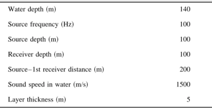
In the example 1, the geoacoustic parameter vector m is formed by the compressional velocities of a five-layer seaf-loor, where each layer has a 5-m thickness. All the other parameters are assumed known and are reported in Table I.
The data vector x is the amplitude of Green’s function at a frequency of 100 Hz, sampled at 64-equally spaced points
in the horizontal wave number space. The undersampling of Green’s function has been considered to resemble the ap-proach of Collins et al.7In the generation of the training and of the test sets, the sound speed in every layer is allowed to vary between 1500 and 2000 m/s. A positive gradient of compressional velocity versus depth is forced, so that the velocity in layer i is always greater than or equal to the velocity in layer i21. Training sets consisting of 50, 100, 200, 400, and 800 pairs, were considered; the same test set of 100 pairs was used in all the above examples.
In evaluating the inversion result, it is important to re-member that we report, for each geoacoustic parameter, the mean error over the whole test set. For this reason, the usual representation of the results ~‘‘true’’ versus ‘‘estimated’’! would not be feasible or even significant in this case.
In Fig. 1 the mean approximation error over the test set is reported for each layer as a function of the number of pairs in the training set. It can be seen that, as expected, the mean error decreases at an increasing in the training set, and that, in the case of a training set of 800 pairs, the error for every layer is below 0.7%. In looking at the result, one has to take into account that, by generating the solution at random ~but with the constraint of positive gradient versus depth!, the relative error is of the order of 10%.
TABLE I. Geometric and environmental information for example 1. The data vector to be inverted is the amplitude of the undersampled Green’s function. The geoacoustic parameters to be retrieved are the compressional wave velocities in five layers of equal thickness. The search interval is 1500–2000 m/s for each layer.
Water depth~m! 140
Source frequency~Hz! 100
Source depth~m! 100
Receiver depth~m! 100
Sound speed in water~m/s! 1500
Layer thickness~m! 5
FIG. 1. Example 1. Mean percentage error over the test set for each layer as a function of the number of pairs in the training set. The number on each curve is referred as to the layer number.
We note, incidentally, that a number of training data of the order of 103 of magnitude is not critical either from the point of view of the network coefficient determination or from the required forward model runs. The generation of the training set of 800 pairs always required less than 2 h on our nonoptimized implementation on an HP 735 workstation with multiple users.
Example 2 was part of a preliminary assessment of the technique for application to the experimental data reported in Sec. III. This explains some of the similarities with the ex-perimental situation. An horizontal towed array of 40 ele-ments, at 4-m spacing, is the receiving system, so the data vector x is in the amplitude of the pressure field at the re-ceivers position. The experimental situation is conceptually similar to that of the sea trial, and is reported in Fig. 2. The source is transmitting a 100-Hz tone signal; the other rel-evant geometrical and environmental parameters ~slightly different from those of the experiment! are reported in Table II.
The bottom was discretized in three layers of 5-m thick-ness each, the geoacoustic model vector to be retrieved was in the compressional and shear velocities for the three layers, and the compressional wave attenuation of the first two lay-ers, for a total of eight parameters. The search spaces for each parameter are reported in Table III.
A training set of 800 pairs was generated, forcing a posi-tive gradient versus depth for both compressional and shear speeds. No assumptions were made for the attenuation. The results over a test set of 100 pairs, generated with the same assumptions used for the training set, are reported in Table IV.
The results of this simulative test show that, at least in this case, the accuracy of the RBF inversion is physically consistent with the relative influence of each parameter on acoustic propagation. One would especially expect the acoustic field to be most sensitive to the compressional ve-locity, to be fairly sensitive to any shear velocity of the order of magnitude of 400 m/s and above, and possibly to show some sensitivity to the compressional attenuation. By look-ing at the results in Table IV, one can see that compressional velocities are all estimated with a mean error of less than 1%; the shear velocity of the third layer, being on the aver-age higher than those of the first two layers~remember that the shear velocity is forced to have a positive gradient w.r. to depth!, is also better retrieved. As for compressional wave attenuation, the standard deviation values show that, in this case, the RBF approximation is not able to produce any meaningful result, confirming the expectation that the acous-tic field is least sensitive to this parameter.
III. FIELD DATA INVERSION
We will now describe the results obtained with the RBF-based inversion on towed array data in a shallow water en-vironment. This data set was acquired during an experiment that took place in February and March 1995 in the Adventure Bank area of the Strait of Sicily in the Mediterannean Sea. The experiment focused on at-sea testing of operational pro-cedures to estimate geoacoustic parameters in shallow water with a moderate aperture towed array. A 40-hydrophone, 4-m spaced, horizontal array was employed, together with a flextensional sound source operated at low frequency in cw mode. Both source and receivers were towed from the same platform at 4 knots, with the geometric configuration of Fig. 2. The relative position of the source-receiving array geom-etry was monitored at regular intervals by acoustic means.
FIG. 2. Experimental configuration of the field experiment.
TABLE II. Geometric and environmental information for example 2. The data vector to be inverted is the amplitude of the pressure field on a 40-element horizontal array. Elements spacing is fixed at 4 m. The geoacoustic parameters to be retrieved are the compressional and shear wave velocity in each layer, plus the compressional wave attenuation in the first two layers.
Water depth~m! 140
Source frequency~Hz! 100
Source depth~m! 100
Receiver depth~m! 100
Source–1st receiver distance~m! 200
Sound speed in water~m/s! 1500
Layer thickness~m! 5
TABLE III. Parameter search space for example 2. The training set has generated by randomly selecting the geoacoustic parameter values in inter-vals noted with the constraint of positive compressional and shear velocity gradients versus depth.
Layer No. P velocity ~m/s! S velocity~m/s! P attenuation~dB/l! 1 1500–1900 80–400 0.1–1 2 1500–2000 80–600 0.1–1 3 1600–3000 150–1500 •••
The deformation of the towed array was constantly moni-tored in real time by means of nonacoustic sensors. Ground truth information was obtained by independent measure-ments through gravity cores, geophone data, and a shallow seismic survey, integrated with Hamilton’s tabulation34 and geological information on the area. The independent geoa-coustic model thus obtained is reported in Table V, together with the relevant water column information. It is important to underline that the information on the last sediment layer was derived through the use of Hamilton regression equa-tions, and not by direct measurements. The sediments in this area are generally described as sandy sediments rich in car-bonate content.
A detailed description of the experiment, including the system setup, will be described elsewhere. A cruise and data report can be found in Ref. 32. For the purpose of the present article, we are satisfied in reporting the results obtained in-verting a subset of the whole data set that can be directly compared with the geoacoustic model of Table V. For this set of data, the acoustic source was transmitting at 110 Hz. As mentioned earlier, the SNR during the experiment was estimated of the order of 20 dB.
The data set to be inverted consisted of 15 ‘‘snapshots,’’ each one the amplitude of the 110-Hz pressure field as re-ceived at the 40 hydrophones. The snapshots were collected at different instants in time during the tow. Before the inver-sion, the data were smoothed with a 4-point moving average. The smoothed data set is reported in Fig. 3.
The 15 snapshots were acquired over a range of 600 m, in an environmental situation that could be fairly described as range independent. However, as can be seen, the data show some relevant variability from one snapshot to the other.
Using the information on the receiver’s position~both in
depth and range!, source depth ~40 m! and source-first re-ceiver distance~535 m!, a RBF inversion network was built with the methodology described in Sec. I and with the same discretization and training rules of example 2 in Sec. II. Note that, although known, we have not included the true layer thickness in order to have a sort of ‘‘blind’’ or semiblind application of the method.
Each of the 15 snapshots was inverted by the same net-work. The results of the inversion for each snapshot were averaged, and the average values, together with the standard deviation, are reported in Table VI. These results can be directly compared with those of the independent Hamilton-based geoacoustic model. Moreover, the standard deviation gives an indication on the variability of the estimates. Note that this variability can be due both to the approximation inherent in the RBF approach and to the variability of the data themselves.
It can be noted that the results obtained are fairly close to that of the independent geoacoustic model, taking into account the differences in methodology. The compressional velocities estimated with the RBF inversion are higher than those of the Hamilton-based model, particularly in the last layer. Note, however, that the RBF estimate is closer to what may be expected for a carbonate sand sediment, and that in the same area it was already reported, at least for shear ve-locity, that there was a discrepancy between Hamilton-based expectations and in situ measured values.24
FIG. 3. Amplitude of the pressure field as received at the hydrophones for the fifteen snapshots.
TABLE IV. Mean relative error and standard deviation of the RBF inversion result over the test set for example 2.
Layer No.
P velocity S velocity P attenuation
Mean~%! s.d.~%! Mean~%! s.d.~%! Mean~%! s.d.~%!
1 0.4 0.3 4.0 6.5 24 86
2 0.7 0.8 7.2 12.8 22 37
3 0.8 1.6 3.3 4.1 ••• •••
TABLE V. Geoacoustic model of the experiment site obtained through in-dependent measurements and Hamilton’s regression curves. Depth is as-sumed 0 at the water surface.
Depth
~m! P velocity~m/s! S velocity~m/s! Description
0–118 1508 0 water column
118–124 1550 230 recent sediments—sand
124–126 1585 275 transition—sand
126–136 1610 290 quaternary sediments—sand
The high values of the standard deviation for the shear velocity are an indication of a poor performance of the in-version scheme or of a strong lateral variability of shear properties in the area ~or both!. It has to be taken into ac-count that the data do display variability, and that perhaps even averaging the estimates on a relatively short path may lead to incorrect conclusions.
For sediment classification purposes, it may be interest-ing to compare the estimated P velocity versus S velocity ratio to those reported by Hamilton.33This was done by con-sidering the ratio of the mean estimates and the maximum and minimum ratio compatible with the standard deviations reported. The results are reported in Fig. 4, together with Hamilton’s curves. Note that we estimate interval velocities for a three-layer model, where each layer has a thickness of 5 m. Note also that again Hamilton’s tabulation holds for fine sand, since he had insufficient data to examine soft, unlithi-fied calcareous sediments.33For consolidated and/or lithified bottoms, Hamilton reports velocity ratios between 1.71 and 2.06, with only one exception at 2.66~see Ref. 33, Table III!. Looking at Fig. 4, it is possible to see that our estimated ratios, even taking into account the relevant standard devia-tion in the shear velocity, allow for an unambigous classifi-cation of at least the second and third layers as unconsoli-dated sediment, slightly harder than water saturated fine sand. By combining this information with the compressional velocity estimates alone and the data in Ref. 34, the sediment
can be classified as a low porosity coarse sand.
IV. DISCUSSION AND CONCLUSION
The RBF approach to geoacoustic inversion was intro-duced, and has proved feasible on simulated data. The first attempt to use this inversion technique on field data has given results that are in qualitative and, to a certain extent, also in quantitative agreement with independent estimates of the same quantities. It has also to be noted that we have not attempted any particular optimization of the RBF procedure tailored to the specific experimental situation. Our purpose here is to show the results of the technique in its standard formulation. We are currently exploring optimization proce-dures with the goal of not loosing, or loosing only in part, the generality and the simplicity of the method.
From the point of view of computational efficiency, the inversion of the fifteen data sets required 900 runs of the forward model ~as many as needed by the training and the test set!, plus the solution of the linear algebraic systems for the coefficient identification. If one wants to compare this with the number of forward model iterations needed for a global search strategy, one has to consider that a new global search should be done for each of the fifteen snapshots in the data set. By using, for instance, the amount of forward model computations reported for typical runs of the genetic algorithms,13 one gets 10 000 runs of forward models for a single search with the standard algorithm, and 1000 runs
~still for a single search! with the hybrid version.
The saving in computational time may seem evident; however care should be taken in comparing the two methods only on the basis of numerical efficiency. The RBF approach is well suited for all applications in which the same experi-mental configuration is used to survey different areas, and particularly if the experimental setup is known in advance. In this case, the network coefficient can be identified before the experiment, and the inversion can be performed in real time. Geophysical surveys with a towed array, like the one of the experiment in Sec. III, are an example of such a situation.
However, one has to remember that, even in the best case, the RBF scheme is inherently an approximation. When accuracy in the result is a critical parameter, global search strategies should still be preferred.
ACKNOWLEDGMENT
This work was supported by European Economic Com-mission under Contract No. MAS2-920022.
1G. V. Frisk and J. F. Lynch, ‘‘Shallow water waveguide characterization
using the Hankel transform,’’ J. Acoust. Soc. Am. 76, 205–216~1984!.
2G. V. Frisk, J. F. Lynch, and J. A. Doutt, ‘‘The determination of
geoa-coustic models in shallow water,’’ in Ocean Seismo-ageoa-coustic, edited by T. Akal and J. M. Berkson~Plenum, New York, 1986!, pp. 693–702.
3
S. D. Rajan, J. F. Lynch, and G. V. Frisk, ‘‘Perturbative inversion meth-ods for obtaining bottom geoacoustic parameters in shallow water,’’ J. Acoust. Soc. Am. 82, 998–1017~1987!.
4G. V. Frisk, ‘‘A review of modal inversion methods for inferring
geoa-coustic properties in shallow water,’’ in Full Field Inversion Methods in
Ocean and Seismo-acoustics, edited by O. Diachok, A. Caiti, P. Gerstoft,
and H. Schmidt~Kluwer, Dordrecht, 1995!, pp. 305–310.
5S. D. Rajan, ‘‘Waveform inversion for geoacoustic parameters of the
TABLE VI. Result of the RBF inversion, averaged over the data set of Fig. 2. Depth ~m! P velocity S velocity Mean ~m/s! s.d. ~m/s! Mean ~m/s! s.d. ~m/s! 118–123 1576 30 184 142 123–128 1660 86 353 140 >128 1850 73 373 154
FIG. 4. Compressional versus shear velocity ratio as a function of depth. Dotted line with stars: inversion results, together with error bars due to the uncertainty in the estimate. Continuous line: typical profile for fine sand ~from Ref. 34 and Table II!. Dotted line: typical profile for silt clay ~from Ref. 34 and Table I!.
ocean bottom in shallow water: matched mode method,’’ in Ref. 4, pp. 299–304.
6M. D. Collins and W. A. Kuperman, ‘‘Focalization: environmental
focus-ing and source localization,’’ J. Acoust. Soc. Am. 90, 1410–1422~1991!.
7M. D. Collins, W. A. Kuperman, and H. Schmidt, ‘‘Nonlinear inversion
for ocean-bottom properties,’’ J. Acoust. Soc. Am. 92, 2770–2783~1992!.
8S. E. Dosso, M. L. Yeremy, K. S. Ozard, and N. R. Chapman,
‘‘Estima-tion of ocean bottom properties by matched field inversion of acoustic field data,’’ IEEE J. Oceanic Eng. 18, 232–239~1993!.
9N. R. Chapman and K. S. Ozard, ‘‘Matched field inversion for geoacoustic
properties of young oceanic crust,’’ in Ref. 4, pp. 165–170.
10P. Gerstoft, ‘‘Inversion of seismo-acoustic data using genetic algorithms
and a posteriori probability distributions,’’ J. Acoust. Soc. Am. 95, 770– 782~1994!.
11M. Lambert, P. Gerstoft, A. Caiti, and R. Ambjornesen, ‘‘Estimation of
bottom parameters from real data by genetic algorithms,’’ in Ref. 4, pp. 159–164.
12
D. F. Gingras and P. Gerstoft, ‘‘Inversion for geometric and geoacoustic parameters in shallow water: experimental results,’’ J. Acoust. Soc. Am.
97, 3589–3598~1995!.
13M. D. Collins and L. Fishman, ‘‘Efficient navigation of parameter
land-scapes,’’ J. Acoust. Soc. Am. 98, 1637–1644~1995!.
14
C. Siedenburg, N. Lehtomaki, J. Arvelo, K. Rao, and H. Schmidt, ‘‘Itera-tive full-field inversion using simulated annealing,’’ in Ref. 4, pp. 121– 126.
15S. M. Jesus and A. Caiti, ‘‘Estimating geoacoustic bottom properties from
towed array data,’’ J. Comp. Acoust.~to be published!.
16P. Gerstoft, ‘‘Inversion of acoustic data using a combination of genetic
algorithms and the Gauss–Newton approach,’’ J. Acoust. Soc. Am. 97, 2181–2190~1995!.
17
P. Gerstoft and A. Caiti, ‘‘Acoustic estimation of bottom parameters: error bounds by local and global methods,’’ in Proceedings of the 2nd
Euro-pean Conference on Underwater Acoustics, edited by L. Bjorno
~Euro-pean Commission, Brussels, 1994!, pp. 887–892.
18H. Schmidt and A. B. Baggeroer, ‘‘Physics-imposed resolution and
ro-bustness issues in seismo-acoustic parameter inversion,’’ in Ref. 4, pp. 121–126.
19G. Roth and A. Tarantola, ‘‘Neural networks and inversion of seismic
data,’’ J. Geophys. Res. B 99, 6753–6768~1994!.
20Y. Stephan, S. Thiria, and F. Badran, ‘‘Application of multilayered neural
networks to ocean acoustic tomography inversion,’’ Report No. 37/95, EPSHOM, Centre Militaire d’ Oceanographie, Brest~1995!.
21
T. Poggio and F. Girosi, ‘‘Networks for approximation and learning,’’ Proc. IEEE 78, 1481–1497~1990!.
22M. J. D. Powell, ‘‘The theory of radial basis functions approximation in
the ’90s,’’ in Advances in Numerical Analysis, edited by W. Light~Oxford U. P., Oxford, 1992!, Vol. II, pp. 105–219.
23
A. Caiti and T. Parisini, ‘‘Mapping ocean sediments by RBF networks,’’ IEEE J. Oceanic Eng. 19, 577–582~1994!.
24A. Caiti, G. Canepa, D. DeRossi, F. Germagnoli, G. Magenes, and T.
Parisini, ‘‘Towards the realization of an artificial tactile system: fine-form discrimination by a tensorial tactile sensor array and neural inversion al-gorithm,’’ IEEE Trans. Syst. Man. Cybern. 25, 933–946~1995!.
25A. Caiti, T. Parisini, and R. Zoppoli, ‘‘Seafloor parameter estimation:
approximating the inverse map through RBF networks,’’ in Ref. 4, pp. 177–182.
26
A. N. Tikhonov and V. Y. Arsenin, Solution of Ill-posed Problems~Wiley, New York, 1977!.
27A. Caiti, T. Akal, and R. D. Stoll, ‘‘Estimation of shear wave velocity in
shallow marrine sediments,’’ IEEE J. Oceanic Eng. 19, 58–72~1994!.
28
T. Poggio and F. Girosi, ‘‘Networks and the best approximation prop-erty,’’ Biol. Cybern. 63, 169–176~1990!.
29H. Schmidt, ‘‘SAFARI: seismo-acoustic fast field algorithm for range
in-dependent environments,’’ SACLANTCEN Report No. SR-113, La Spe-zia~1988!.
30
J. M. Hovem and A. Kristensen, ‘‘Reflection loss at a bottom with a fluid sediment layer over a hard solid halfspace,’’ J. Acoust. Soc. Am. 92, 335–340~1992!.
31S. M. Jesus, ‘‘A sensitivity study for full-field inversion of geoacoustic
data with a towed array in shallow water,’’ in Ref. 4, pp. 103–108.
32
S. M. Jesus, A. Caiti, and H. Zambujo, ‘‘Geophysical seafloor exploration with a towed array in shallow water,’’ 24-month progress report, DG-XII,
ECC~December 1994!.
33E. L. Hamilton, ‘‘V
p/Vs and Poisson’s ratio in marine sediments and rocks,’’ J. Acoust. Soc. Am. 66, 1093–1101~1979!.
34E. L. Hamilton, ‘‘Acoustic properties of sediments,’’ in Acoustics and Ocean Bottom, edited by R. Lara-Saenz, C. Ranz-Guerra, and C.