Abstract
Owing to its particular characteristics, the direct discretization of the Dirac-delta function is not feasible when point discretization methods like the differential quadrature method (DQM) are ap-plied. A way for overcoming this difficulty is to approximate (or regularize) the Dirac-delta function with simple mathematical tions. By regularizing the Dirac-delta function, such singular func-tion is treated as non-singular funcfunc-tions and can be easily and directly discretized using the DQM. On the other hand, it is possi-ble to combine the DQM with the integral quadrature method (IQM) to handle the Dirac-delta function. Alternatively, one may
use another definition of the Dirac-delta function that the
deriva-tive of the Heaviside function, H(x), is the Dirac-delta function,
(x), in the distribution sense, namely, dH(x)/dx = (x). This ap-proach has been referred in the literature as the direct projection approach. It has been shown that although this approach yields highly oscillatory approximation of the Dirac-delta function, it can yield a non-oscillatory approximation of the solution. In this paper,
we first present a modified direct projection approach that
elimi-nates such difficulty (oscillatory approximation of the Dirac-delta function). We then demonstrate the applicability and reliability of the proposed method by applying it to some moving load problems of beams and rectangular plates.
Keywords
DQM, Dirac-delta function, Heaviside function, modified direct projection approach, moving load problem, beams, rectangular plates.
A Differential Quadrature Procedure with Direct Projection
of the Heaviside Function for Numerical Solution of Moving
Load Problem
S.A. Eftekhari *
Young Researchers and Elite Club, Karaj Branch, Islamic Azad University, Karaj, P.O. Box 31485-313, Iran
*Author email:
http://dx.doi.org/10.1590/1679-78252251
1 INTRODUCTION
The differential quadrature method (DQM), which was firstly introduced by Bellman and his asso-ciates (1971, 1972) in the early 1970s, is a powerful numerical method for the direct solution of par-tial differenpar-tial equations that arise in various fields of engineering, mathematics, and physics (Bert and Malik, 1996a; 1996b; Malik and Bert 1996; Tornabene et al., 2015a; Eftekhari 2016a). It is sim-ple to use and also straightforward to imsim-plement. However, in spite of its many desirable features, the DQM is well-known to have some difficulty when applied to partial differential equations in-volving singular functions like the Dirac-delta function. This is mainly caused by the fact that the Dirac-delta function cannot be directly discretized by the DQM.
A way for overcoming the above-mentioned difficulty is to approximate (or regularize) the Di-rac-delta function with simple mathematical functions. By regularizing the DiDi-rac-delta function, such singular function is treated as non-singular functions and can be easily and directly discretized using the DQM. Jung (2009), Jung and Don (2009), Jung et al. (2009), Wang et al. (2014), Eftek-hari (2015a), and Tornabene et al. (2015b) have successfully applied this technique in conjunction with the point discretization methods to solve various partial differential equations involving the Dirac-delta function. However, this technique involves a regularization parameter that should be carefully adjusted before the problem being solved. This parameter has also been shown to be a
problem-dependent parameter (Eftekhari, 2015a).
On the other hand, Eftekhari (2015b, 2016b) proposed a combined application of the DQM and integral quadrature method (IQM) to handle the Dirac-delta function in vibration problem of beams and rectangular plates subjected to a moving (or static) point load. In this combined ap-proach, the particular properties of the Dirac-delta function are taken into account by application of the IQM. The coupled DQM/IQM approach has been shown to be highly accurate and reliable. However, this approach requires the help of another method (i.e., the IQM) to treat the Dirac-delta function. In general, it is more desirable to solve such type of problems by the DQM itself, not by combining the DQM with other methods or techniques.
Alternatively, Jung (2009), Jung and Don (2009) also Jung et al. (2009) made use of an alterna-tive definition of the Dirac-delta function that the derivative of the Heaviside function, H(x), is the Dirac-delta function, (x), in the distribution sense, namely, dH(x)/dx = (x). The method was referred to as the direct projection method. It has been shown that although the direct projection of the Heaviside function gives highly oscillatory approximation of the Dirac-delta function, it can yield a non-oscillatory approximation of the solution and the error can also decay uniformly for certain types of differential equations. Recently, Wang et al. (2014) studied at length various ways of approximation of the Dirac-delta function. They considered the sine-Gordon equation with im-pulsive forcing and concluded that the domain decomposition method is the best among the meth-ods considered in their study.
In this study, a differential quadrature procedure based on the direct projection of the Heaviside function is proposed for the numerical solution of moving load problem, wherein the motion of the point load is described by a time-dependent Dirac-delta function. Since the original direct projection approach shows some oscillations for approximation of the Dirac-delta function, we also introduce a
beams and rectangular plates. Numerical results are presented and compared with analytical and numerical results available in the literature. The numerical results prove that the proposed method is reliable and accurate and can be used as an efficient tool for handling the moving load problem.
2 DQM
Let w(η) be an arbitrary function and η1, η2, …, ηn be a set of grid points in the η-direction. Accord-ing to the DQM, the rth-order derivative of the function w(η) at any grid point can be approximat-ed by the following formulation
nj
j r ij i
r η A wη
w
1 ) ( )
( ( ) ( )
(1)
where w(ηj) represents the function value at a grid point ηj, w
(r)(η
i) indicates the rth-order
deriva-tive of w(η) at a grid point ηi, and (r)
ij
A are the weighting coefficients of the rth-order derivative. The first-order weighting coefficients, i.e., (1)
ij
A , are given by (Quan and Chang, 1989)
n i
k i A
n k
i k i
η η η η
A n
i j j
ij k k i
i
ik
,..., 2 , 1 ,
,..., 2 , 1 , , ) ( ) (
) (
, 1
) 1 ( )
1 (
(2)
where
n
i j j
j i
i η η
η , 1
) ( )
( (3)
The weighting coefficients of the higher-order derivatives (r > 1) can be computed from the fol-lowing recurrence relationship (Bert and Malik, 1996a)
, ] [ ] [ ] [ ] [ ]
[A(r) A(r1)A(1) A(1)A(r1)
r 1 (4)
In this work, the DQM grid points are taken nonuniformly spaced and are given by the follow-ing equations (Bert and Malik, 1996a)
0
1
η , η2Δ, ηn11Δ, ηn1
3 ) 2 ( cos 1 2 / 1
n
π
i
ηi , i3,4,...,n2, 0η 1
where Δ is a parameter that determines the closeness between the boundary points (η1 and ηn) and their immediate adjacent points (η2 and ηn-1). In practice, the magnitude of Δ should be as small as
possible (≤ 10-3). In this study, the magnitude of parameter Δ is assumed to be Δ= 10-3.
3 DIRECT PROJECTION APPROACH
As we discussed before in introduction, the direct discretization of the Dirac-delta function using point discretization methods like the DQM is not feasible. This is mainly due to particular charac-teristics of the Dirac-delta function. For instance, the one-dimensional Dirac-delta function has the following characteristics:
0 )
(xx0 for all x x0 (6)
)d 1
(x x0 x (7)
)d ( )
( )
(x x x0 x f x0
f (8)
where f(x) may be any arbitrary function. As we mentioned in introduction, there has been a con-siderable effort to overcome this difficulty. In this paper, we have tried to solve this difficulty by the help of direct projection of the Heaviside function. The details of this approach will be given in the following sub-sections.
3.1 Approximation of the One-dimensional Dirac-delta Function
3.1.1 Conventional Approach
The direct projection approach is based on the fact that the derivative of the Heaviside function is the Dirac-delta function in the distribution sense, namely,
) ( d
d )
( 0 H 0 x
x x
x x (9)
where Hx0(x) is the Heaviside function defined as (Jung, 2009)
0 0 0
0
, 1 , 2 / 1
, 0 ) (
x x
x x
x x x
Hx (10)
By the help of above definition, the Dirac-delta function can now be directly and simply discre-tized using the DQM. Let x1, x2, …, xn be a set of grid points in the x-direction. Application of the DQM to Eq. (9) gives
} { ] [ }
{δ A(1) H
where [A](1) is the DQM weighting coefficient matrix of the first-order derivative, and
T
n x
x x
x x
x ) ( ) . . . ( )]
( [ }
{δ 1 0 2 0 0 (12)
T n x x
x x H x H x
H ( ) ( ) . . . ( )]
[ }
{H 0 1 0 2 0 (13)
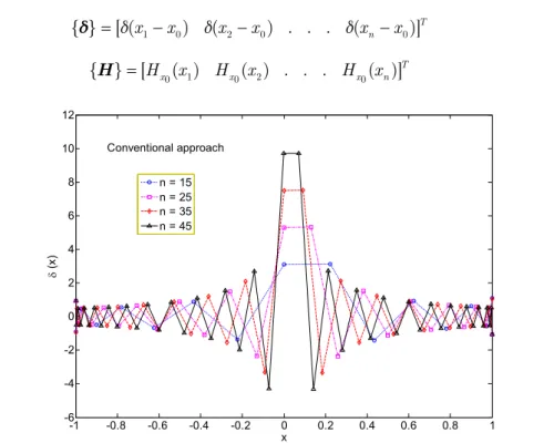
Figure 1: Approximation of the one-dimensional Dirac-delta function using conventional direct projection approach.
Figure 1 shows the results of conventional direct projection approach for approximation of the Dirac-delta function for different number of grid points (n). The coordinates of the grid points are calculated using xicos
π(i1) (n1)
(i 1,2,...,n). As it can be seen, the results of thisap-proach are high oscillatory. The amplitude of the oscillation becomes even more remarkable near the singular point (x = 0). This trend of solutions has also been reported earlier by Jung (2009) and Jung et al. (2009).
3.1.2 Proposed Approach
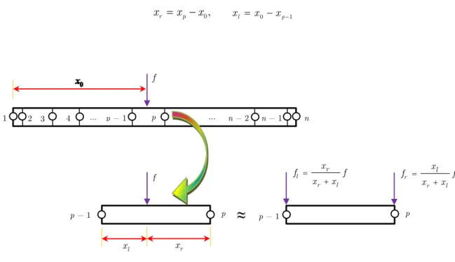
One of the main limitations of the conventional direct projection approach is that the case of arbi-trary location of the singular point (x0) cannot be accurately handled using this approach. Even if the location of the singular point being very close to one of the DQM grid points, this approach is found to show remarkable oscillation for approximation of the Dirac-delta function (see Figure 1). This limitation can be overcome if the weighted distribution of the source point is considered on the two nearest nodes around it (see Figure 2). By doing so, the following definition can be introduced for the Dirac-delta function
), ( )
( )
( 0 1 p
l r
l p
l r
r x x
x x
x x
x x x
x x
x
xp1 x0 xp (14)
where
-1 -0.8 -0.6 -0.4 -0.2 0 0.2 0.4 0.6 0.8 1 -6
-4 -2 0 2 4 6 8 10 12
x
(x)
,
0
x x
xr p xl x0 xp1 (15)
Figure 2: Representation of a point source by two statically equivalent point sources at its adjacent grid points.
Now, introducing Eq. (9) to Eq. (14) gives
) ( d d ) ( d d )
( 0 1 H x
x x x x x H x x x x x
x xp
l r l p x l r r
(16)
where , , 1 , 2 / 1 , 0 ) ( 1 1 1 1 p p p p x x x x x x x x H p p p p x x x x x x x x H , 1 , 2 / 1 , 0 ) ( (17)
Application of the DQM to Eq. (16) gives
[ ] { } { } }
{ (1) R
l r l L l r r x x x x x
x H H
A
δ (18)
where {δ} is defined already in Eq. (12) and
T n p x p x p x L x H x H x
H ( ) ( ) . . . ( )]
[ }
{H 1 1 1 2 1 (19)
T n p x p x p x R x H x H x
H ( ) ( ) . . . ( )]
[ }
{H 1 2 (20)
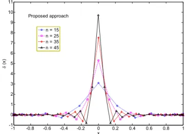
When above definition is used, Figure 3 illustrate the results. Comparing these results with those of Figure 1, one sees that the proposed method gives much better approximation for the Di-rac-delta function as compared with the conventional direct projection approach. The amplitude of
r
x
l
x
p p − 1
p p − 1
… p −1 p n−2
f x x x f l r l r f
… n−1 n
oscillations is damped out considerably. However, there are some small amplitude oscillations near the singular point which are known to be due to the Gibbs phenomenon (for more details about this phenomenon see Myint-U (1980, 2007)).
Figure 3: Approximation of the one-dimensional Dirac-delta function using proposed direct projection approach.
3.2 Approximation of the Two-Dimensional Dirac-Delta Function
The approaches presented in previous section (section 3.1) can be easily extended to discretize the two-dimensional Dirac-delta function. The details are given in the following sub-sections.
3.2.1 Conventional Approach
Using Eq. (9), the two-dimensional Dirac-delta function can be expressed as
) ( d
d ) ( d
d ) ( ) ( ) ,
( 0 0 0 0 0 H0 y
y x H x y y x x y y x
x x y (21)
where Hx0(x) is defined in Eq. (10) and
0 0 0
0
, 1 , 2 / 1
, 0 ) (
y y
y y
y y y
Hy (22)
Consider n grid points with coordinates x1, x2, …, xn in the x-direction, and m grid points with coordinates y1, y2, …, ym in the y-direction. Application of the DQM to Eq. (21) gives
T T x y m T
x y T x y
] } { . . . } { } { [ } ~
{δ 1 δ 2 δ δ (23)
where
-1 -0.8 -0.6 -0.4 -0.2 0 0.2 0.4 0.6 0.8 1 -1
0 1 2 3 4 5 6 7 8 9 10 11
x
(x)
( ) ( ) ( )
[ ] { } }{ (1)
0 0 2 0 1 x T n x x x x x x
x A H
δ (24)
( ) ( ) ( )
[ ] { }}
{ (1)
0 0 2 0 1 y T m y y y y y y
y A H
δ (25)
wherein [A](1) and [A](1)are the first-order DQM weighting coefficient matrices associated with the
x- and y-derivatives, respectively. Furthermore,
T n x x
x
x} [H (x ) H (x ) . . . H (x )]
{H 0 1 0 2 0 (26)
T m y y
y
y} [H (y ) H (y ) . . . H (y )]
{H 0 1 0 2 0 (27)
3.2.2 Proposed Approach
Let xp1 x0 xp and yq1 y0 yq.Using Eqs. (9) and (14), the two-dimensional Dirac-delta
function can be expressed as
, ) ( ) ( )
(x x0 y y0 x x0 y y0
( 1) ( ) ( 1) ( q)
l r l q l r r p l r l p l r
r y y
y y y y y y y y x x x x x x x x x x
d ( )
d ) ( d d ) ( d d ) ( d d 1
1 y y yH y
y y H y y y y x H x x x x x H x x x x q y l r l q y l r r p x l r l p x l r r (28)
where xr, xl, Hxp1(x)andHxp(x) are defined in Eqs. (15) and (17). Furthermore,
,
0
y y
yr q yl y0 yq1 (29)
, , 1 , 2 / 1 , 0 ) ( 1 1 1 1 q q q q y y y y y y y y H q q q q y y y y y y y y H , 1 , 2 / 1 , 0 ) ( (30)
Now, application of the DQM to Eq. (28) gives
T T x y m T x y T x
y{ } { } . . . { } ]
[ } ~
{δ 1 δ 2 δ δ (31)
( ) ( ) ( ) [ ] { } { } }{ (1)
0 0 2 0 1 R x l r l L x l r r T n x x x x x x x x x x x x
x A H H
δ (32)
where
( ) ( ) ( ) [ ] { } { } }{ (1)
0 0 2 0 1 R y l r l L y l r r T m y y y y y y y y y y y y
y A H H
δ (33)
wherein T n p x p x p x L
x} [H (x ) H (x ) . . . H (x )]
T n p x p
x p
x R
x} [H (x ) H (x ) . . . H (x )]
{H 1 2 (35)
T m q y q
y q
y L
y} [H (y ) H (y ) . . . H (y )]
{H 1 1 1 2 1 (36)
T m q y q
y q
y R
y} [H (y ) H (y ) . . . H (y )]
{H 1 2 (37)
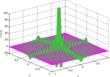
In Figures 4 and 5 the results of proposed approach are compared with those of conventional approach for approximation of the two-dimensional Dirac-delta function. These results are obtained using n = m = 51. The results of the conventional approach are observed to be highly oscillatory. The results of the proposed approach, however, do not show such an oscillatory behavior.
Figure 4: Approximation of the two-dimensional Dirac-delta function using conventional direct
projection approach (n = m = 51).
Figure 5: Approximation of the two-dimensional Dirac-delta function using proposed direct
projection approach (n = m = 51).
-1 -0.5
0 0.5 1
-1 -0.5 0 0.5 1 -20 0 20 40 60 80 100
x y
(x,
y)
-1 -0.5
0 0.5 1
-1 -0.5 0 0.5 1 -20 0 20 40 60 80 100
x y
4 FORMULATION FOR FORCED VIBRATION OF BEAMS CARRYING MOVING LOADS
Consider an Euler-Bernoulli beam with length L, mass per unit length ρA, and bending stiffness EI
subjected to a point load f moving at a constant velocity v. The governing differential equation of motion of the beam is given by (Meirovitch, 1967; Fryba, 1999)
)), ( ( ) , ( )
, (
4 4 2
2
t x x f x
t x w EI t
t x w A
ρ f
xf(t)vt (38)
where w(x, t) is the transverse deflection of the beam, and xf(t) is the position coordinate of the moving point load.
Consider n grid points with coordinates x1, x2, …, xn in the x-direction. In view of Eq. (16), Eq.
(38) can be rewritten as (xp1 xf(t) xp)
d ( )
d )
( d
d )
, ( )
, (
1 4
4 2
2
x H x x x
x x H x x x
x f x
t x w EI t
t x w A
ρ xp
l r
l p
x l r
r
(39)
Satisfying Eq. (39) at any grid point x = xi (i = 1, 2, …, n) and substituting the quadrature rule into results gives
)} ( { )} ( ]{ [ )} ( ]{
[M W t K Wt Ft (40)
where [M] and [K]are the mass and stiffness matrices of the beam,{W(t)}and{W(t)}are the
displacement and acceleration vectors, and{F(t)}is the load vector. [M], [K], {W(t)},{W(t)}and
)} (
{Ft are given by (
p f
p x t x
x 1 () )
], [ ]
[M ρAI [K]EI[A](4) (41)
T
n t
x w t
x w t x w
t)} [ ( , ) ( , ) . . . ( , )] (
{W 1 2 (42)
T
n t
x w t
x w t x w
t)} [ ( , ) ( , ) . . . ( , )]
(
{W 1 2 (43)
f t)} (
{F
{ } { }
]
[ (1) R
l r
l L
l r
r
x x
x x
x x
H H
A (44)
where [I] is an identity matrix of order n × n, [A](r) (r = 1, 4) are the DQM weighting coefficient
matrix of the rth-order derivative, and the matrices {HL} and {HR} are defined already in Eqs.
(19) and (20). It should be noted that since the position of the moving point load changes from time to time, the variables xr and xl are time-dependent variables. For the same reason, the vectors
}
{HL and {HR} are time-dependent vectors. As a result, the load vector { ()}
t
F is also a
time-dependent vector.
5 FORMULATION FOR FORCED VIBRATION OF RECTANGULAR PLATES CARRYING MOVING LOADS
Consider a rectangular thin plate with length a, width b, mass per unit area ρh, and bending rigidi-ty D under a moving point load f. The governing differential equation of motion of the rectangular plate is given by (Rao, 2007)
)), ( ( )) ( ( 2 4 4 2 2 4 4 4 2 2 t y y t x x f y w y x w x w D t w h
ρ f f
xf(t)vxt, yf(t)vyt (45)
where w(x, y, t) is the transverse deflection of the plate, xf(t) and yf(t) are position coordinates of the moving point load in the x- and y-direction, respectively, and vx and vy are the corresponding
moving speeds.
Consider n grid points with coordinates x1, x2, …, xn in the x-direction, and m grid points with coordinates y1, y2, …, ym in the y-direction. In view of Eq. (28), Eq. (45) can be rewritten as (xp1 xf(t)xp, yq1 yf(t)yq)
4 4 2 2 4 4 4 2 2 2 y w y x w x w D t w h ρ ( ) d d ) ( d d ) ( d d ) ( d d 1
1 y y yH y
y y H y y y y x H x x x x x H x x x x
f yq
l r l q y l r r p x l r l p x l r r (46)
Satisfying Eq. (46) at any grid point x = xi and substituting the quadrature rule1), into results gives )} , ( { ] [ )} , ( { ] [ 2 )} , ( { ] [ )} , ( { ] [ 4 4 2 2 ) 2 ( ) 4 ( 2 2 t y y t y y t y D t y t h
ρ I W A W A W I W
)} ( { ) ( d d ) ( d d
1 y y yH y t
y y H y y y y x q y l r l q y l r r F (47)
where [I] is an identity matrix of order n × n, and [A](r) (r = 2, 4) are the DQM weighting
coeffi-cient matrices of the rth-order x-derivative. Furthermore,
T
n yt
x w t y x w t y x w t
y, )} [ ( , , ) ( , , ) . . . ( , , )]
(
{W 1 2 (48)
[ ] { } { } )} (
{ (1) R
x l r l L x l r r x x x x x x x f
t A H H
F (49)
where the matrices { L}
x
H and { R} x
H are defined in Eqs. (34) and (35).
Satisfying Eq. (47) at any grid point y = yi and substituting the quadrature rule into results gives
)} ( ~ { )} ( ~ ]{ ~ [ )} ( ~ ]{ ~
where [M~] and [K~]are the mass and stiffness matrices of the plate, {W~(t)}and{W~(t)}are the
displacement and acceleration vectors, and{F~(t)}is the load vector. The n × n sub-matrices [ ~ ]
ij
M
and [K~ij], and the n × 1sub-vector {F~i}are given by
], [ ]
~
[M I
ij
ij ρhI i,j 1,2,...,m (51)
[ ] 2 [ ] [ ]
]~
[K A(4) (2)A(2) (4)I
ij ij
ij
ij DI A A (52)
} { } ~
{ y x
i
i F F
F (53)
where Iij are the elements of m × m identity matrix, and
) (r ij
A (r = 2, 4) are the DQM weighting coefficients of the rth-order y-derivative. Furthermore,
T T m T
T
t y t
y t
y
t)} [{ ( , )} { ( , )} . . . { ( , )} ]
( ~
{W W 1 W 2 W (54)
T T m T
T
t y t
y t
y
t)} [{ ( , )} { ( , )} . . . { ( , )} ]
( ~
{W W 1 W 2 W (55)
[ ] { } { }
)} (
{ (1) R
y l r
l L y l r
r y
y y
y y
y y
t A H H
F (56)
where the matrices { L} y
H and { R} y
H are defined in Eqs. (36) and (37). It should be noted that
since the location of the moving load changes from time to time, the variables xr, xl, yr, and yl also the vectors { L}
x
H , { R} x
H , { L} y
H and { R} y
H are time-dependent.
After applying the plate boundary conditions, one can solve the resulting system of ordinary dif-ferential equations for unknowns using various time integration schemes. The details of implemen-tation of the plate boundary conditions can be found in Malik and Bert (1996) and also in Eftekhari (2015c). In this study, the Newmark method (Bathe and Wilson, 1976) is employed to solve Eqs. (40) and (50).
6 NUMERICAL RESULTS AND DISCUSSION
To validate the proposed formulation and its implementation, a number of numerical examples are now presented. The first and second examples demonstrate the applications of the proposed method to static analysis of beams and rectangular plates subjected to point loads. These numerical exam-ples are presented herein to better verify the accuracy and convergence of the method. The same problems are considered in the third and fourth examples, but the location of the point load is as-sumed to vary with time.
6.1 Deflection of a Simply Supported Beam Due to a Concentrated Point Load
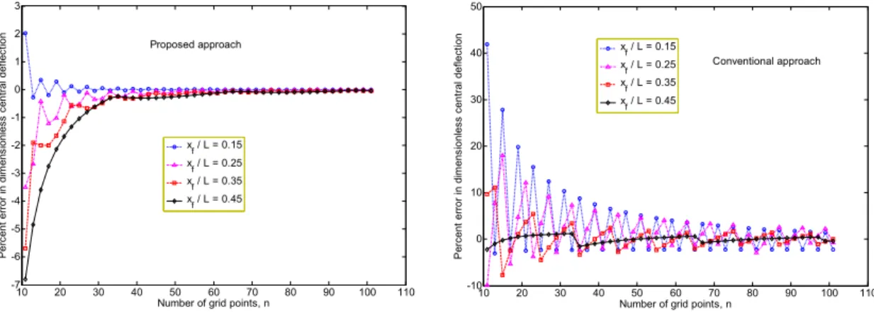
using the conventional approach are also shown for comparison purposes. It can be seen that the results of proposed approach converge uniformly to their final values. The results of the convention-al approach, however, are somewhat erratic and their behavior is somehow oscillatory.
In Figure 7 the results of proposed approach are compared with those of the DQMR (DQM with regularized Dirac-delta function). The DQMR results are shown for three different values of α. It is noted that in DQMR, the Dirac-delta function is approximated as (Eftekhari, 2015a)
2
2
α
) ( exp
α
1 )
( f
f
x x
π
x
x (57)
where α is the regularization parameter. It can be seen from Figure 7 that the results of the DQMR is highly dependent on the values of α. For large values of α, the results of the DQMR are not very accurate, and for small values of this parameter the DQMR solutions show some oscillation for small number of grid points. The results of the proposed approach are found to be better than those of the DQMR in terms of both accuracy and convergence.
Figure 6: Convergence and accuracy of the dimensionless central deflection (w/ , = fL3/EI) of a simply supported beam subjected to a point load for different locations of the applied load.
Figure 7: Comparison of the dimensionless deflection (w/ , = fL3/EI) of a simply supported beam subjected to a point load for different locations of the applied load.
10 20 30 40 50 60 70 80 90 100 110
-7 -6 -5 -4 -3 -2 -1 0 1 2 3
Number of grid points, n
Pe
rc
en
t e
rror
in
dim
ens
io
nle
ss
c
en
tra
l d
ef
lec
tio
n
xf / L = 0.15 xf / L = 0.25 xf / L = 0.35 xf / L = 0.45 Proposed approach
10 20 30 40 50 60 70 80 90 100 110
-10 0 10 20 30 40 50
Number of grid points, n
Pe
rc
en
t e
rro
r i
n
dim
en
si
on
le
ss
c
en
tral
de
fle
ct
ion xf / L = 0.15
xf / L = 0.25 xf / L = 0.35 xf / L = 0.45
Conventional approach
10 15 20 25 30 35 40 45 50 55
-35 -30 -25 -20 -15 -10 -5 0
Number of grid points, n
Pe
rc
en
t e
rror
in
dim
ens
io
nle
ss
c
en
tra
l d
ef
lec
tio
n
DQMR ( = 0.1) DQMR ( = 0.075) DQMR ( = 0.05) Proposed approach
xf / L = 0.45
10 15 20 25 30 35 40 45 50 55
-30 -20 -10 0 10 20 30 40 50 60
Number of grid points, n
Pe
rc
en
t er
ro
r in
d
im
en
si
on
le
ss
c
en
tra
l d
ef
lec
tio
n
DQMR ( = 0.1) DQMR ( = 0.075) DQMR ( = 0.05) Proposed approach
6.2 Deflection of a Simply Supported Rectangular Plate Due to a Concentrated Point Load
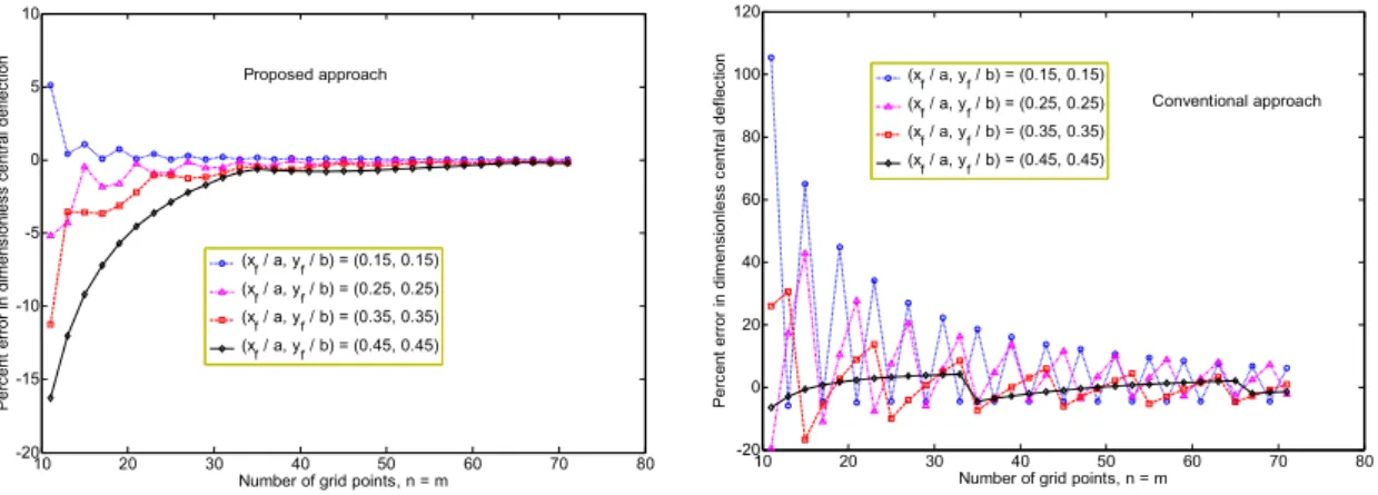
Consider the bending problem of a simply supported rectangular plate subjected to a concentrated point load f acting at a point (x, y) = (xf, yf). Figure 8 shows the convergence and accuracy of the dimensionless central deflection of the plate for different locations of the applied load. It can be seen that the results by present method show better convergence trend than the conventional approach. On the other hand, by comparing these results with those of Figure 6, one sees that the behavior of solutions in this case (plate problem) is very similar to that of the beam problem. The only differ-ence is that the order of error in solutions of the plate problem is larger than that of the beam prob-lem.
In Figure 9 the results are compared with those of the DQMR. Again, one sees that the results of proposed approach are better than those of the DQMR in terms of both accuracy and conver-gence.
Figure 8: Convergence and accuracy of the dimensionless central deflection (w/ , = fa2/D) of a simply supported square plate subjected to a point load for different locations of the applied load.
Figure 9: Comparison of the dimensionless deflection (w/ , = fa2/D) of a simply supported square plate subjected to a point load for different locations of the applied load.
10 20 30 40 50 60 70 80
-20 -15 -10 -5 0 5 10
Number of grid points, n = m
Pe
rc
en
t er
ro
r in
d
im
en
si
on
le
ss
c
en
tra
l d
ef
lec
tio
n
(xf / a, yf / b) = (0.15, 0.15) (xf / a, yf / b) = (0.25, 0.25) (xf / a, yf / b) = (0.35, 0.35) (xf / a, yf / b) = (0.45, 0.45)
Proposed approach
10 20 30 40 50 60 70 80
-20 0 20 40 60 80 100 120
Number of grid points, n = m
Pe
rc
en
t e
rror
in
dim
ens
io
nle
ss
c
en
tra
l d
ef
lec
tio
n
(xf / a, yf / b) = (0.15, 0.15) (xf / a, yf / b) = (0.25, 0.25) (xf / a, yf / b) = (0.35, 0.35) (xf / a, yf / b) = (0.45, 0.45)
Conventional approach
10 15 20 25 30 35 40 45 50 55
-60 -40 -20 0 20 40 60 80 100 120 140
Number of grid points, n = m
Pe
rc
en
t e
rror
in
dim
ens
io
nle
ss
c
en
tra
l d
ef
lec
tio
n
DQMR ( = 0.1) DQMR ( = 0.075) DQMR ( = 0.05) Proposed approach
(xf / a, yf / b) = (0.15, 0.15)
10 15 20 25 30 35 40 45 50 55
-60 -50 -40 -30 -20 -10 0
Number of grid points, n = m
Pe
rc
en
t e
rror
in
dim
ens
io
nle
ss
c
en
tra
l d
ef
lec
tio
n
DQMR ( = 0.1) DQMR ( = 0.075) DQMR ( = 0.05) Proposed approach
6.3 Vibration of a Beam Due to a Moving Point Load
Consider the vibration problem of a simply supported beam subjected to a moving point load. The parameters of the problem are assumed to be (Eftekhari, 2015a):
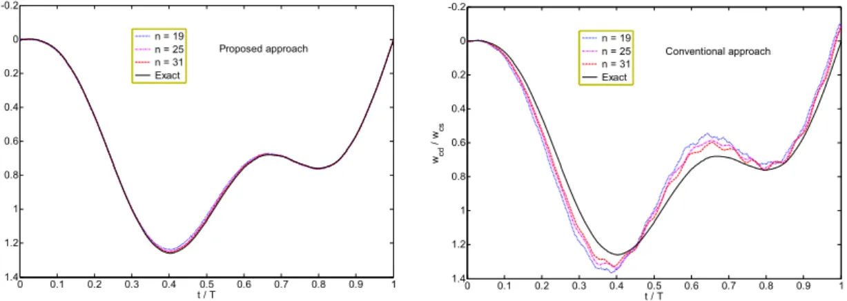
ρ = 10686.9 kg/m3, b = 0.635 cm, h = 0.635 cm, E = 2.068 × 10¹¹ Pa, L = 10.16 cm, f = 4.45 N where b and h are the width and thickness of the beam. The dynamic central deflections of the beam, wcd, are evaluated for different values of moving speed (v) and normalized by the static de-flection wcs = fL3/(48EI). Figures 10 and 11 present the convergence of solutions for different load speeds. The results are also compared with those obtained using the conventional approach. It can be seen from Figures 10 and 11 that the results generated by the proposed method converge rapidly to their final values and agree well with analytical solutions. The results of the conventional ap-proach, however, are highly oscillatory and erratic. Note that the error in solutions of the conven-tional approach never decays even if a large number of grid points are used. This implies that the conventional approach is not suitable for studying the moving load-type problems.
Figure 10: Convergence and accuracy of numerical results for normalized central deflection of a simply
supported beam subjected to a moving point load (v = 31.2 m/s).
Figure 11: Convergence and accuracy of numerical results for normalized central deflection of a
simply supported beam subjected to a moving point load (v = 62.4 m/s).
0 0.1 0.2 0.3 0.4 0.5 0.6 0.7 0.8 0.9 1
1.2 1 0.8 0.6 0.4 0.2 0 -0.2
t / T
wcd
/ w
cs
n = 19 n = 25 n = 31 Exact
Proposed approach
0 0.1 0.2 0.3 0.4 0.5 0.6 0.7 0.8 0.9 1
1.2 1 0.8 0.6 0.4 0.2 0 -0.2
t / T
wcd
/ w
cs
n = 19 n = 25 n = 31 Exact
Conventional approach
0 0.1 0.2 0.3 0.4 0.5 0.6 0.7 0.8 0.9 1
1.4 1.2 1 0.8 0.6 0.4 0.2 0 -0.2
t / T
wcd
/ w
cs
n = 19 n = 25 n = 31 Exact
Proposed approach
0 0.1 0.2 0.3 0.4 0.5 0.6 0.7 0.8 0.9 1
1.4 1.2 1 0.8 0.6 0.4 0.2 0 -0.2
t / T
wcd
/ w
cs
n = 19 n = 25 n = 31 Exact
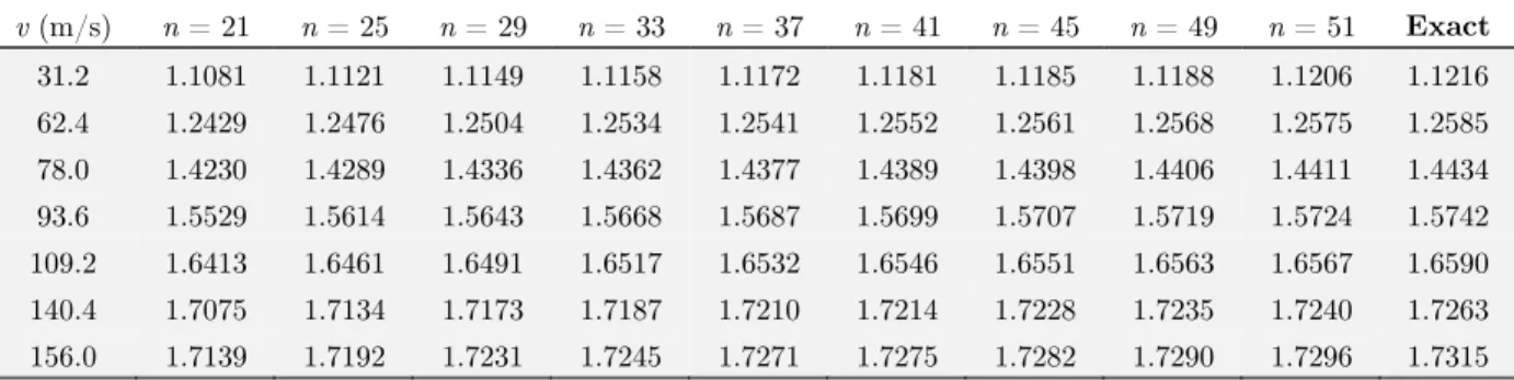
In Table 1, the numerical results are given for dynamic magnification factors (DMFs) (maxi-mum value of normalized deflection at the beam center) of a simply supported beam for different values of moving speed. The analytical solution values are also shown for comparison. It can be seen from Table 1 that the results of proposed approach converge uniformly to those of exact solution as the number of grid points increases. Besides, they agree very closely with analytical solution values. In Table 2, the results of proposed approach are compared with those of other DQM procedures.
v (m/s) n = 21 n = 25 n = 29 n = 33 n = 37 n = 41 n = 45 n = 49 n = 51 Exact
31.2 1.1081 1.1121 1.1149 1.1158 1.1172 1.1181 1.1185 1.1188 1.1206 1.1216
62.4 1.2429 1.2476 1.2504 1.2534 1.2541 1.2552 1.2561 1.2568 1.2575 1.2585
78.0 1.4230 1.4289 1.4336 1.4362 1.4377 1.4389 1.4398 1.4406 1.4411 1.4434
93.6 1.5529 1.5614 1.5643 1.5668 1.5687 1.5699 1.5707 1.5719 1.5724 1.5742
109.2 1.6413 1.6461 1.6491 1.6517 1.6532 1.6546 1.6551 1.6563 1.6567 1.6590
140.4 1.7075 1.7134 1.7173 1.7187 1.7210 1.7214 1.7228 1.7235 1.7240 1.7263
156.0 1.7139 1.7192 1.7231 1.7245 1.7271 1.7275 1.7282 1.7290 1.7296 1.7315
Table 1: Convergence and accuracy of DMFs of a simply supported beam subjected to a moving point load for different load speeds.
v (m/s) Present
(n = 25)
Present
(n = 35)
Present
(n = 51)
DQMR
(n = 25)
DQMR
(n = 35)
DQMR
(n = 51)
DQM/IQM (n
= 25) Exact
31.2 1.1121 1.1170 1.1206 1.1793 1.1168 1.1220 1.121 1.1216
62.4 1.2476 1.2536 1.2575 1.3337 1.2691 1.2550 1.257 1.2585
78.0 1.4289 1.4372 1.4411 1.4878 1.4503 1.4414 1.441 1.4434
109.2 1.6461 1.6523 1.6567 1.6767 1.6582 1.6591 1.658 1.6590
Table 2: Comparison of DMFs of a simply supported beam subjected to a moving point load for different load speeds.
It can be seen from Table 2 that the results generated by the DQMR are somewhat oscillatory. Note that the results of this approach with n = 25 are erroneous. By increasing the number of grid points, however, the DQMR results approach to the exact solution results. Compared with the DQMR approach, the proposed approach provides better convergence and, in most cases, leads to better accuracy. The DQM/IQM approach is found to be more efficient than other two approaches. But, this approach requires the help of another method (i.e., the IQM) to treat the Dirac-delta function, and this is not very desirable.
Now consider a clamped beam under a moving point load. The numerical results for this case are given in Table 3 together with the finite element solution results of Rieker et al. (1996). Note that, in this case, the central deflections of the beam are normalized by the static deflection wcs =
DQM/IQM approach are found to have closer agreement with the finite element solution results of Rieker et al. (1996).
v (m/s) n = 25 n = 29 n = 33 n = 37 n = 41 n = 45 n = 49 n = 51 Rieker et al. (1996)
141.3070 1.282 1.289 1.294 1.297 1.300 1.301 1.303 1.305 1.311
282.6140 1.616 1.621 1.626 1.629 1.631 1.632 1.633 1.635 1.637
423.9210 1.541 1.540 1.544 1.545 1.546 1.548 1.548 1.548 1.552
Table 3: Convergence and accuracy of DMFs of a clamped beam subjected to a moving concentrated load for different load speeds.
v (m/s) Present
(n = 31)
Present
(n = 39)
DQMR
(n = 31)
DQMR
(n = 39)
DQM/IQM
(n = 31)
Rieker et al. (1996)
141.3070 1.291 1.298 1.308 1.303 1.304 1.311
282.6140 1.624 1.630 1.630 1.636 1.634 1.637
423.9210 1.541 1.546 1.548 1.549 1.549 1.552
Table 4: Comparison of DMFs of a clamped beam subjected to a moving point load for different load speeds.
6.4 Vibration of a Rectangular Plate Due to a Moving Point Load
Consider a simply supported rectangular plate subjected to a moving point load. The plate and load parameters are assumed to be (Eftekhari, 2015a):
ρh/D = 1, f/D = 1, a = b = 1, xf(t) = vt, yf(t) = constant = ½
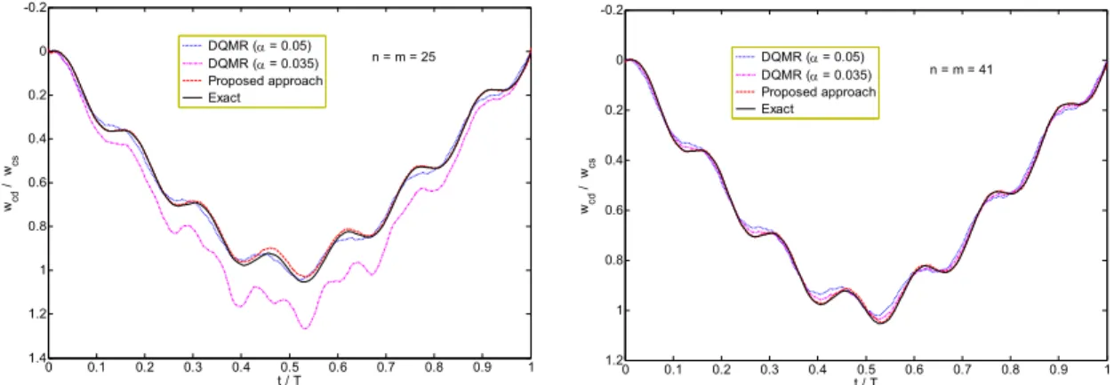
Figure 12 illustrates the convergence of solutions and Figure 13 presents a comparison of the re-sults with the DQMR rere-sults.
Figure 12: Convergence and accuracy of numerical results for normalized central deflection of a simply supported rectangular plate subjected to a moving point load.
0 0.1 0.2 0.3 0.4 0.5 0.6 0.7 0.8 0.9 1 1.2
1 0.8 0.6 0.4 0.2 0 -0.2
t / T wcd
/ w
cs
n = m = 25 n = m = 33 n = m = 41 Exact
v = 0.45 m/s
0 0.1 0.2 0.3 0.4 0.5 0.6 0.7 0.8 0.9 1 1.6
1.4 1.2 1 0.8 0.6 0.4 0.2 0 -0.2
t / T wcd
/ w
cs
n = m = 25 n = m = 33 n = m = 41 Exact
Figure 13: Comparison of numerical results for normalized central deflection of a simply supported rectangular
plate subjected to a moving point load (v = 0.45 m/s).
It can be seen from Figure 12 that the computed solutions converge monotonically to the exact solutions as the number of grid points increases. Convergence is also more rapid when the moving speed is high. Figure 13 shows again the better performance of the proposed approach over the DQMR approach. Note that the DQMR approach may produce erroneous results with small num-ber of grid points (n = m = 25) when the value of the regularization parameter (α) is too small (α = 0.035). Although this can be avoided by increasing the number of grid points (see the results correspond to n = m = 41), the regularization parameter should be carefully adjusted before the problem being solved. In the proposed approach, there is no need to adjust any parameter before solving the problem. Therefore, the proposed approach is more straightforward to implement than the DQMR approach.
7 CONCLUSIONS
The direct discretization of the Dirac-delta function using point discretization techniques like the DQM is not an easy task and special treatment is required. A way for overcoming this difficulty is to use an alternative definition of the Dirac-delta function that the derivative of the Heaviside func-tion in the distribufunc-tion sense is the Dirac-delta funcfunc-tion. This approach has been referred in the literature as the direct projection approach. The conventional direct projection approach, however, shows some oscillations for approximation of the Dirac-delta function. To overcome this limitation, this paper introduces a modified direct projection approach that provides better approximation for the Dirac-delta function while eliminates such difficulty. The applicability and reliability of the proposed method are demonstrated herein through solution of some moving load problems of beams and rectangular plates. The proposed approach is shown to be superior over the DQMR approach in terms of both accuracy and convergence.
References
Bathe, K.J., Wilson, E.L. (1976). Numerical Methods in Finite Element Analysis. Prentice-Hall, Englewood Cliffs (New Jersey).
0 0.1 0.2 0.3 0.4 0.5 0.6 0.7 0.8 0.9 1
1.4 1.2 1 0.8 0.6 0.4 0.2 0 -0.2
t / T
wcd
/ w
cs
DQMR ( = 0.05) DQMR ( = 0.035) Proposed approach Exact
n = m = 25
0 0.1 0.2 0.3 0.4 0.5 0.6 0.7 0.8 0.9 1
1.2 1 0.8 0.6 0.4 0.2 0 -0.2
t / T
wcd
/ w
cs
DQMR ( = 0.05) DQMR ( = 0.035) Proposed approach Exact
Bellman, R.E., Casti, J. (1971). Differential quadrature and long term integration. J Math Anal Appl 34: 235–238. Bellman, R.E., Kashef, B.G., Casti, J. (1972). Differential quadrature: A technique for the rapid solution of nonlinear partial differential equations. J Comput Phys 10: 40–52.
Bert, C.W., Malik, M. (1996a). Differential quadrature method in computational mechanics: A review. ASME Appl Mech Rev 49: 1–28.
Bert, C.W., Malik, M. (1996b). The differential quadrature method for irregular domains and application to plate vibration. Int J Mech Sci 38(6): 589-606.
Eftekhari, S.A. (2015a). A differential quadrature procedure with regularization of the Dirac-delta function for nu-merical solution of moving load problem. Latin American J Solids Struct 12: 1241-1265.
Eftekhari, S.A. (2015b). A note on mathematical treatment of the Dirac-delta function in the differential quadrature bending and forced vibration analysis of beams and rectangular plates subjected to concentrated loads. Appl Math Model 39: 6223–6242.
Eftekhari, S.A. (2015c). A simple and systematic approach for implementing boundary conditions in the differential quadrature free and forced vibration analysis of beams and rectangular plates. J Solid Mech 7(4): 374-399.
Eftekhari, S.A. (2016a). Pressure-based and potential-based mixed Ritz-differential quadrature formulations for free and forced vibration of Timoshenko beams in contact with fluid. Meccanica 51:179–210.
Eftekhari, S.A. (2016b). A modified differential quadrature procedure for numerical solution of moving load problem. Proc IMechE Part C: J Mech Eng Sci 230(5): 715–731.
Fryba, L. (1999). Vibration of Solids and Structures under Moving Loads. Thomas Telford (London).
Jung, J-H. (2009). A Note on the spectral collocation approximation of some differential equations with singular source terms. J Sci Comput 39: 1573–7691.
Jung, J-H., Don, W.S. (2009). Collocation methods for hyperbolic partial differential equations with singular sources. Adv Appl Math Mech 1(6):769-780.
Jung, J-H., Khanna, G. Nagle, I. (2009). A spectral collocation approximation for the radial-infall of a compact ob-ject into a Schwarzschild black hole. Int J Mod Phys C 20:1–22.
Malik, M., Bert, C.W. (1996). Implementing multiple boundary conditions in the DQ solution of higher-order PDE’s:
application to free vibration of plates. Int J Numer Meth Eng39:1237-1258.
Meirovitch, L. (1967). Analytical Methods in Vibrations. Macmillan (New York).
Myint-U, T. (1980). Partial Differential Equations of Mathematical Physics. 2nd ed. North-Holland (New York) Myint-U, T., Debnath, L. (2007). Linear Partial Differential Equations for Scientists and Engineers. 4th ed. Birkhäu-ser (Boston)
Quan, J.R., Chang, C.T. (1989). New insights in solving distributed system equations by the quadrature methods, Part I: analysis. Comput Chem Eng 13:779–788.
Rao, S.S. (2007). Vibration of Continuous Systems. John Wiley & Sons, Inc. (New Jersey).
Rieker, J. R., Lin, Y.-H., Trethewey, M. W. (1996). Discretization considerations in moving load finite element beam models. Finite Elem Anal Design 21: 129–144.
Tornabene, F., Fantuzzi, N., Ubertini, F., Viola, E. (2015a). Strong formulation finite element method: a survey.
ASME Appl Mech Rev 67:020801.
Tornabene, F., Fantuzzi, N., Bacciocch, M., Viola, E. (2015b) A new approach for treating concentrated loads in doubly-curved composite deep shells with variable radii of curvature. Compos Struct 131: 433-452.