Spinning rough disc moving in a rarefied
medium
BY ALEXANDER PLAKHOV1,2,*, TATIANA TCHEMISOVA2 AND PAULO GOUVEIA3 1University of Aberystwyth, Aberystwyth SY23 3BZ, Ceredigion, UK
2University of Aveiro, Aveiro 3810-193, Portugal
3Polytechnic Institute of Bragança, Bragança 5301-854, Portugal
We study the Magnus effect: deflection of the trajectory of a spinning body moving in a gas. It is well known that in rarefied gases, the inverse Magnus effect takes place, which means that the transversal component of the force acting on the body has opposite signs in sparse and relatively dense gases. The existing works derive the inverse effect from non-elastic interaction of gas particles with the body. We propose another (complementary) mechanism of creating the transversal force owing to multiple collisions of particles in cavities of the body surface. We limit ourselves to the two-dimensional case of a rough disc moving through a zero-temperature medium on the plane, where reflections of the particles from the body are elastic and mutual interaction of the particles is neglected. We represent the force acting on the disc and the moment of this force as functionals depending on ‘shape of the roughness’, and determine the set of all admissible forces. The disc trajectory is determined for several simple cases. The study is made by means of billiard theory, Monge–Kantorovich optimal mass transport and by numerical methods.
Keywords: inverse Magnus effect; free molecular flow; rough surface; billiards; optimal mass transport
1. Introduction
We are concerned here with the Magnus effect: the phenomenon governing deflection of the trajectory of spinning bodies (e.g. golf ball or football). Surprisingly enough, in highly rarefied media (on Mars or in the thin atmosphere at a height corresponding to low earth orbits, 150 km or more), the inverse effect takes place; this means that the trajectory deflection has opposite signs in sparse and in dense media.
Actually, all these models ignore roughness, which is always present on the body’s surface. The kind of the roughness (that is, the shape of microscopic dimples, hollows, gullies, etc.) depends on the body material; the surface may also be artificially roughened. Owing to the roughness, particles bounce off the body surface in directions other than that prescribed by the visible orientation of the surface, and may also have multiple reflections.
We believe that roughness of the body surface should be incorporated in the model and propose a new approach to studying the Magnus effect. This approach is based on examining the shape of the body’s cavities and is applied to a very idealized case of a two-dimensional rough disc, where all reflections are supposed to be elastic.
This approach meets evident difficulties: there is a huge variety of shapes governing the roughness. The existing literature deals with many different kinds of roughness: Gaussian, non-Gaussian, fractal, etc. Each of them provides the special kind of reflection law, which may be very hard to determine. The difficulty of the task seems to be immense.
Fortunately, there is an easier way to get rid of these difficulties. Instead of calculating the scattering law for each given roughness, a sort of inverse problem can be considered: determine the set of scattering laws for all possible shapes of roughness. The main tool for this approach has been developed by Plakhov (2009a). Having solved this problem, we are in a position to determine the main characteristic of the effect: the range of forces acting on the body and of the moments of these forces. Of relatively less importance, but quite illustrative, is the calculation of forces and trajectories for several special kinds of roughness.
We warn the reader against seeing this paper as directly applicable to real-life cases. Rather, it provides an insight into studying the cases of complex surfaces. The next steps in this way would be application of this approach to three-dimensional bodies and allowing for non-elastic reflections.
Another novelty of our paper consists in applying optimal mass transport (OMT), a very vivid and rapidly growing field of calculus of variations (see Rachev & Rüschendorf (1998) and Villani (2003) for a review of the progress in this theory), to the study of the inverse Magnus effect. A sort of vector-valued OMT problem naturally appears and is examined here. To the best of our knowledge, this kind of generalization of OMT has never been considered before. This paper is a further development of the ideas briefly reported byPlakhov & Tchemisova (2009).
We now proceed to a detailed description of the problem. A spinning two-dimensional body moves through a homogeneous medium on the plane. The medium is extremely rarefied, so that the free path length of particles is much larger than the body’s size. In such a case, the interaction of the body with the medium can be described in terms of free molecular flow, where point particles fall on the body’s surface and each particle interacts with the body, but not with the other particles. There is no gravitation force. The particles of the medium remain at rest; that is, the absolute temperature of the medium equals zero. In a frame of reference moving forward together with the body, we have a parallel flow of particles falling on the body at rest (figure 1).
w
B
Figure 1. A rotating rough disc in a parallel flow of particles.
The body under consideration is a rough disc, that is, a set obtained from a circle by making infinitely small dimples on its boundary. More precisely, consider a sequence of sets Bm, m=3, 4, 5,. . ., inscribed in the circle Br(O) of radius r centred at a point O. Each set Bm is invariant under the rotation by the angle 2p/m, and the intersection of Bm with a certain (2p/m)-sector AmOCm formed by two radii OAm and OCm is a set bounded by these radii and by a piecewise smooth non-self-intersecting curve contained in the triangle AmOCm and joining the points Am and Cm. These curves are similar for all m.1 A rough disc B is associated with such a sequence of sets Bm. The curve is called the shape of roughness. All the values related to resistance or dynamics of the rough disc that are calculated below are understood as limits of the corresponding values for Bm as m→ ∞.
Note in passing that the roughness introduced here is uniform: it is identical at each point of the circle boundary. In the case of non-uniform roughness, that is, if the shape of dimples varies along the boundary, periodical oscillations of the disc along the trajectory may happen, the period being equal to the period of one turn of the disc. The ‘averaged’ trajectory, however, coincides with the trajectory of the uniformly rough disc, where the roughness is obtained by ‘averaging’ the original one.
Denote by4(t) the rotation angle at the time t, byu(t) the angular velocity of the disc,u(t)=d4/dt, and letv(t) be the velocity of the disc centre of mass. Let us agree to measure the rotation angle and the angular velocity counterclockwise. We consider the following problems: (A) determine the force of the medium resistance acting on the disc, find the moment of this force with respect to the disc centre of mass and investigate their dependence on the shape of roughness; (B) determine the set of admissible forces; and (C) analyse the motion of rough discs in the medium, that is, study the behaviour of the functions u(t) and v(t). Problems (A) and (B) are primary with respect to (C). In the paper, we will devote the main attention to problems (A) and (B), having just touched upon problem (C), where we will restrict ourselves to deducing equations of motion and solving these equations for several simple cases.
R
RL RL
RT R
T
R
v v
(a) (b)
Figure 2. (a) The Magnus effect; (b) the inverse Magnus effect.
With each set Bm, we associate a distribution of mass inside Bm such that the total massM is constant and the centre of the mass coincides with the centreO of the set. We also assume that the moment of inertia Im of Bm about O converges to a positive value I as m→ ∞. One always has I ≤Mr2. Denote b=Mr2/I; that is, b is the inverse relative moment of inertia; we have 1≤b<+∞. In what follows, we will pay special attention to two particular cases: (i)b=1, the mass of the disc is concentrated near its boundary, and (ii)b=2, the mass is distributed uniformly in the disc.
The resistance force Rm(Bm,4,u,v) acting on the set Bm and the moment of this force RI,m(Bm,4,u,v) depend on the shape of roughness, the rotation angle 4, the angular velocity u and the velocity of translation v. The equations of dynamics are
Mdv
dt =Rm(Bm,4,u,v), Im du
dt =RI,m(Bm,u,v) and d4
dt =u.
Taking the limit m → ∞, one gets the resistance force acting on the rough disc R(B,u,v) and the moment of this force RI(B,u,v), which do not depend on 4 anymore, and the equations for the disc dynamics take the form
Mdv
dt =R(B,u,v) (1.1)
and
Idu
dt =RI(B,u,v). (1.2)
We shall see below that, generally speaking, R=R(B,u,v) is not collinear to v.
If a transversal component of the resistance force appears, resulting in deflection of the body’s trajectory, then we encounter the (proper or inverse) Magnus effect. If the direction of the transversal component coincides with the instantaneous velocity of the front point of the body, then a proper Magnus effect takes place. If these directions are opposite, then an inverse Magnus effect occurs (figure 2a,b).
I3
I2
I1
W3 W2
W1
Wi x
x+ j+ j
D
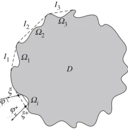
Figure 3. Cavities on the boundary of a non-convex set.
In the next section, to each rough discB, we assign a measurenB characterizing the law of billiard scattering on B. The values R and RI are defined to be functions of the valuesnB,uandv. In §3, we define the set of all possible values of R, when u and v are fixed and nB takes all admissible values. In other words, we answer the following question: what is the range of values of the force acting on a rough disc? While we look through all possible shapes of roughness, the vector R covers a fixed convex two-dimensional set. The problem of finding this set is formulated in terms of a special vector-valued Monge–Kantorovich problem and is solved numerically for several fixed values of the parameter l=ur/v. Further, we calculate R and RI for some special values of nB (and thus for some special kinds of rough bodies). In §4, we deduce the equations of dynamics in a convenient form and solve them in several simple particular cases. Finally, in §5, a comparison of our results with those of the previous works on the inverse Magnus effect in rarefied media is given.
2. Law of billiard scattering and resistance
(a)Billiard scattering by a non-convex set
Let us first define the measure nD characterizing billiard scattering on a bounded simply connected set D⊂R2 with a piecewise smooth boundary. The set v(convD)\vD= ∪i≥1Ii is the union of a finite or countable family of connected
components Ii,i=1, 2,. . .. Each component Ii is an open interval. (In figure 3,
the dashed line denotes the intervals Ii, i=1, 2, 3.) Denote I0=v(convD)∩vD;
in other words,I0 is the ‘convex part’ of the boundaryvD. Thus,vD is the disjoint
union vD= ∪i≥0Ii.
Further, the set convD\D is the union of a finite or countable collection of its connected components. For any Ii, there exists a set Ui from this collection such that Ii⊂vUi (figure 3). The pair (Ui,Ii) will be called a cavity, and the interval Ii, the opening of the cavity.
Denote by nx the outer unit normal to v(convD) at the point x∈v(convD). On the set Ii × [−p/2,p/2] with the coordinates (x,4), define the measure
one-dimensional Lebesgue measure. Consider the billiard in R2\D. Fix x∈Ii and 4∈ [−p/2,p/2], and take a billiard particle that starts moving at the point x with the velocity forming the angle 4 with −nx. The particle makes one or several reflections at points of vUi \Ii and then intersects Ii once again at the point x+=x+i (x,4), the velocity at the moment of intersection forming the angle 4+=4+i (x,4) with the vector nx+,4+∈ [−p/2,p/2]. Notice that one always has nx=nx+. In figure 3, we have 4<0 and 4+=4+
i (x,4)>0.
Thus, for each i, we have defined the mapping (x,4)→(x+i ,4+i ) from a full measure subset of Ii × [−p/2, p/2] onto itself. This mapping is a bijection and involution, and preserves the measure mi. In the particular case, where i=0, it holds x+0 =x and 40+= −4. Denote by li = |Ii| the length of Ii, and by l =
i≥0li = |v(convD)| the perimeter of convD. Introduce the notation
✷:= [−p/2,p/2] × [−p/2,p/2] and define the measures niD, i=0, 1, 2,. . . on ✷
as follows: nDi (A) :=(1/li)mi({(x,4) : (4,4+i (x,4))∈A}) for any Borel set A⊂✷. In particular, the measure n0D=:n0 is supported on the diagonal 4+= −4, and has the density dn0(4,4+)=cos4·d(4+4+). Finally, define nD:=1/l
i≥0liniD. The measure nD is called law of billiard scattering by D.
In a less formal way, the measure nD can be interpreted as follows. Place the body D in a kind of ‘ether’ and keep it motionless. By ether, we mean a homogeneous isotropic medium composed of mutually non-interacting particles moving freely with unit velocity in all possible directions. When colliding with the body, the particles reflect elastically from its boundary. Thus, the particles of the ether behave like billiard particles in R2\D.
For each particle that has reflected from D, fix the pair (4,4+) of the angle of incidence 4 and the angle of reflection 4+. The angle 4 is formed by the initial velocity of the particle and the vector −nx, whereas the angle 4+ is formed by its final velocity and the vector nx+. Here, xand x+ are the points of the first and second intersection of the particle’s trajectory with v(convD). The distribution of the set of pairs (4,4+) for all particles that have collided with D in a unit time period is described by the measure nD.
Recall that given a Borel mapping p:X →Y of two sets X ⊂Rd1, Y ⊂Rd2,
with the setX being equipped with a Borel measurem, the so-called push-forward measure p#m on Y is defined by p#m(A) :=m(p−1(A)) for any Borel set A⊂Y. Denote by p4 and p4+ :✷→ [−p/2, p/2] the projections of the square ✷ on its
horizontal and vertical sides, respectively; p4(4,4+)=4, p4+(4,4+)=4+. The
push-forward measuresp#4nandp#4+nare called marginal measures forn. They are defined on[−p/2, p/2], and for any Borel set A⊂ [−p/2, p/2]we havep#4n(A)=
n(A× [−p/2, p/2]), p4#+n(A)=n([−p/2, p/2] ×A).
Define the transformation of the square pd :✷→✷ exchanging the coordinates
4 and 4+; that is, pd(4,4+)=(4+,4). The push-forward measure pd#n satisfies the condition pd#n(A)=n(pd(A)) for any Borel set A⊂✷. In other words, the measurespd#n andnare mutually symmetric with respect to the diagonal 4=4+. Finally, define the measure g on [−p/2, p/2] by dg=cos4d4, and denote by
Psymm the set of measures n on ✷ satisfying the conditions
x
wr
n
x −v
j
Figure 4. A particle falling on a cavity.
In other words, a generic measure from Psymm is symmetric with respect to the
diagonal 4=4+, and both of its marginal measures coincide with g. One has nDi ∈Psymm; this can be easily deduced from the measure preserving and involutive
properties of the mapping (x,4)→(x+i ,4+i ); for details seePlakhov (2004). Hence,
nD ∈Psymm. Moreover, the following fundamental theorem characterizing the set of scattering laws holds true (Plakhov 2009a).
Theorem 2.1. Whatever the two sets K1⊂K2⊂R2such thatdist(vK1,vK2)>0, the set of measures {nD :K1⊂D⊂K2} is everywhere dense in Psymm in the weak topology.
Now consider the rough disc B generated by a sequence of sets Bm. All the cavities of all the sets Bm are similar; therefore, nBm does not depend on m and we can set by definition nB:=nBm. We will see later that the resistance of B can be written down as a functional of nB. The following theorem is obtained by a slight modification of the proof of theorem 2.1.
Theorem 2.2. Whatever r >0, the set {nB:B is a rough disc of radius r} is everywhere dense in Psymm in the weak topology.
(b)Resistance of a rough disc
Denotev= |v|and choose the (non-inertial) frame of referenceOx1x2 such that the direction of the axisOx2 coincides with the direction of the disc motion and the origin O coincides with the disc centre. In this frame of reference, the disc stays at rest, and the flow of particles falls down on it at the velocity −v0=(0;−v)T. Here and in what follows, we represent vectors as columns; for instance, a vector x will be denoted by
x1 x2
or (x1;x2)T.
Let us calculate the force R of the medium resistance and the moment of this force RI with respect to O. To that end, first we consider the pre-limit body Bm. Parametrize the opening of each cavity by the variable x varying from 0 to 1 (recall that all the cavities are identical). Denote by r the flow density, by 4, the rotation angle of the cavity (that is, the external normal at the cavity opening equals nx=(−sin4; cos4)T) and by v+
Dt=2p/(um) is the minimal time period between two identical positions of the
rotating setBm. Then the momentum imparted toBm by the particles of the flow during the time interval Dt equals
2rrvDt
1
0
p/2
−p/2
(−v0−v+
(m)(x,4)) 1
2cos4d4dx, (2.2)
Consider the frame of reference O˜x˜1x˜2 having the centre at the midpoint of the cavity opening I; the axis O˜x˜1 being parallel to I; and O˜x˜2, codirectional with nx. That is, the frame of reference rotates jointly with the segment I. The change of variables from x =(x1;x2)T to x˜ =(x˜1;x˜2)T and the inverse one are given by x˜ =A−utx −r cos(p/m)ep/2 and x =Autx˜ +r cos(p/m)ep/2+ut, where Af=
cosf −sinf sinf cosf
and ef=
cosf sinf
.
Suppose now that x(t) and x˜(t) are the coordinates of a moving point in the initial and rotating frames of reference, respectively, and letv=(v1;v2)T=dx/dt and v˜ =(v˜1;v˜2)T=dx˜/dt. Then,
˜
v=A−utv−uAp/2−utx and v=Autv˜ +uAp/2+utx˜ −ur cosp m
eut. (2.3)
We apply formulae (2.3) to the velocity of the particle at the two moments of its intersection withI. At the first moment, it holds ut=4andx =rep/2+4 +o(1) as m→ ∞. (Here and in what follows, the estimateso(1) are not necessarily uniform with respect to x and 4.) Then the incidence velocity −v0 takes the form
− ˜v0=v(l−sin4;−cos4)T+o(1)= −v9(−sinx; cosx)T+o(1), (2.4) where l=ur/v and
9=9(4,l)= l2−2lsin4+1 and x =x(4,l)=arcsinl−sin4
9(4,l) . (2.5) As m → ∞, the time spent by the particle in the cavity tends to zero; therefore, the rotating frame of reference can be considered ‘approximately inertial’ during that time, and the velocity at the second point of intersection is given by v˜+=v9(−siny; cosy)T+o(1), where y=y(x,4,l)=4+(x,x(4,l)). (Here x+(x,4), 4+(x,4) denote the mapping generated by the cavity; §2a) Applying the second formula in equation (2.3) and taking into account that
˜
x=o(1) and ut=4+o(1), we find the velocity in the initial frame of reference, v+=v+
(m)(x,4,l)=v9A4(−siny; cosy)T −vle4 +o(1)=v+(x,4,l)+o(1), where
v+(x,4,l)=v
−9sin(4+y)−lcos4 9cos(4+y)−lsin4
Letting m→ ∞ in formulae (2.2) for the imparted momentum and dividing it by Dt, we get the following formula for the force of resistance acting on the disc:
R=
RT RL
=rrv
1
0
p/2
−p/2
(−v0−v+(x,4,l)) cos4dxd4. (2.7) The angular momentum transmitted to Bm by an individual particle equals rv9(sinx +siny)+o(1) times the mass of the particle. Summing the angular momenta up over all incident particles and passing to the limit m→ ∞, one finds the moment of the resistance force acting on the disc,
RI =r2rv
1
0
p/2
−p/2
v9(4,l)(sinx(4,l)+siny(x,4,l)) cos4dxd4. (2.8) Theorem 2.3. The resistance and the moment of resistance of a rough disc of radius r moving through a rarefied medium are equal to
R= 8
3rrv 2
·R[nB,l] (2.9)
and
RI = 8 3r
2rv2
·RI[nB,l]. (2.10)
Here r is the medium density, v is the velocity of translation, u is the angular velocity, l=ur/v and the dimensionless values R[n,l] and RI[n,l] are given by the integral formulas
R[n,l] =
RT[n,l] RL[n,l]
=
✷
c(x,y,l) dn(x,y), (2.11) and
RI[n,l] =
✷
cI(x,y,l) dn(x,y), (2.12) with the functions c and cI given by the relations (2.13)–(2.20). Recall that ✷= [−p/2,p/2] × [−p/2,p/2]. We also use the notation z=z(x,l)= arcsin√1−l2cos2x and x
0=x0(l)=arccos 1/l; c stands for the characteristic function.
(a) If 0<l≤1, then
c(x,y,l)= 3 4
(lsinx +sinz)3 sinz cos
x −y 2 ⎡ ⎢ ⎢ ⎢ ⎣ cos
z+ x −y 2
−sin
z+ x −y 2 ⎤ ⎥ ⎥ ⎥ ⎦ (2.13) and
cI(x,y,l)= − 3 8
(lsinx +sinz)3
and in particular,
c(x,y, 1)=3 sin2x
cos(2x −y)+cosx −sin(2x −y)−sinx
cx≥0(x,y) (2.15)
and
cI(x,y, 1)= −3 sin2x(sinx +siny)cx≥0(x,y). (2.16) In the limiting case l→0+, one has
c(x,y,l)= −3 8
sin(x −y) 1+cos(x −y)
+O(l) (2.17)
and
cI(x,y)= 9l
8 sinx(sinx +siny)+O(l
2). (2.18)
(b) If l>1, then
c(x,y,l)= 3 2
cos(x −y)/2 sinz ⎧ ⎪ ⎨ ⎪ ⎩
(l3sin3x +3lsinxsin2z) cosz
⎡
⎢ ⎣
cos x −y 2 −sin x −y
2
⎤
⎥ ⎦
− (3l2sin2xsinz+sin3z) sinz
⎡
⎢ ⎣
sinx −y 2 cosx −y
2 ⎤ ⎥ ⎦ ⎫ ⎪ ⎬ ⎪ ⎭
cx≥x0(x,y) (2.19)
and
cI(x,y,l)= −3 4
l3sin3x +3lsinxsin2z
sinz (sinx +siny)cx≥x0(x,y). (2.20) Proof. The theorem will be proved separately for cases l=1, 0<l<1 and l>1.
Case l=1. We have x=x(4, 1)=arcsin (1−sin4)/2=p/4−4/2, and so, the function 4→x(4, 1) is a bijection between the intervals [−p/2,p/2] and [0,p/2]. Further, one has 9=9(4, 1)= 2(1−sin4)=2 sinx, cos4=sin 2x, and we get from equation (2.6) that v+=v
−2 sinx cos(2x −y)−sin 2x 2 sinxsin(2x −y)−cos 2x
, wherefrom −v0−v+=2vsinx
cos(2x −y)+cosx −sin(2x −y)−sinx
. Making the change of variables{x,4} → {x,x} in the integral in equation (2.7) and using equation (2.9), one gets
R[nB, 1] =3
1
0
p/2
0
sin2x
cos(2x −y)+cosx −sin(2x −y)−sinx
In this integral, y is the function of x and x, y=4+(x,x). Changing the variables once again, {x,x} → {x,y}, and taking into account that cosxdxdx =dnB(x,y), we obtain
R[nB, 1] =3
sin2x
cos(2x −y)+cosx −sin(2x −y)−sinx
dnB(x,y). (2.21)
Here the symbol stands for the rectangle x ∈ [0,p/2], y∈ [−p/2,p/2]. The moment of the resistance force is calculated analogously, resulting in
RI[nB, 1] = −3
1
0
p/2
0
sin2x(sinx +siny) cosx dxdx
= −3
sin2x(sinx +siny)dnB(x,y). (2.22)
Case 0<l<1. The second relation in equation (2.5) implies that for a fixed value of l, x =x(4,l) is a monotone decreasing function of 4 that varies from p/2 to −p/2 as 4 changes from −p/2 to p/2. From formulae (2.4) and the first relation in equation (2.5), we have sin4=lcos2x −sinx√1−l2cos2x, cos4= cosx(lsinx +√1−l2cos2x), 9=lsinx +√1−l2cos2x. Recall that
z=z(x,l)=arcsin 1−l2cos2x; (2.23) one has cosz=lcosx,x +z=p/2−4,z∈ [arccosl,p/2], and taking into account equation (2.6), we get −v0−v+=v(lsinx +sinz)·2 cos(x −y)/2
cos(z+(x −y)/2) −sin(z+(x −y)/2)
, cos4/cosx =lsinx +sinz=9 and d4/dx = −1−dz/dx = −(lsinx +sinz)/sinz.
Using the obtained formula, making the change of variables {x,4} → {x,x} in the integral (2.7), and taking into account equation (2.9), one gets
R[nB,l] =3 4
1
0
p/2
−p/2
(lsinx +sinz)3 sinz cos
x −y 2 ⎡ ⎢ ⎢ ⎣ cos
z+ x −y 2
−sin
z+ x −y 2 ⎤ ⎥ ⎥ ⎦
cosx dxdx.
Finally, the change of variables {x,x} → {x,y} results in
R[nB,l] = 3
4 ✷
(lsinx +sinz)3 sinz cos
x −y 2 ⎡ ⎢ ⎢ ⎣ cos
z+ x −y 2
−sin
z+ x −y 2 ⎤ ⎥ ⎥ ⎦
dnB(x,y).
In a similar way, from equation (2.8), one gets RI = −
3 8
1
0
p/2
−p/2
(lsinx +sinz)3
sinz (sinx +siny) cosx dxdx; wherefrom
RI[nB,l] = − 3
8 ✷
(lsinx +sinz)3
sinz (sinx +siny) dnB(x,y). (2.25) Formulae (2.21) and (2.22) are the particular cases of equations (2.24) and (2.25) for l=1. This can be easily verified taking into account that z(x, 1)= |x|. Case l>1. In this case, x=x(4,l) equation (2.5) is not injection any more. When4varies from−p/2 to40=40(l) :=arcsin 1/l, the value ofx monotonically decreases fromp/2 to x0=x0(l)=arccos 1/l, and when 4 varies from 40 to p/2, x monotonically increases from x0 to p/2. Denote by 4−:=4−(x,l) and 4+:=
4+(x,l) the functions inverse to x(4,l) on the intervals [−p/2,40] and[40,p/2], respectively. Then, one has sin4±=lcos2x ±sinx√1−l2cos2x.
Here and in what follows, the signs ‘+’ and ‘−’ are related to the functions 4+ and 4− respectively. The values 4+, 4− and z=z(x,l) equation (2.23) satisfy the relations p/2−4+=x −z,p/2−4−=x +z. The function z is defined for x∈ [x0,p/2] and monotonically increases from 0 to p/2, when x changes in the interval [x0,p/2].
After some algebra, one gets cos4±/cosx =sin(x ∓z)/cosx =lsinx ∓ sinz; ±d4±/dx =dz/dx ∓1=lsinx ∓sinz/sinz; 9±=lsinx ∓sinz; −v0− v+
±=v(lsinx ∓sinz)·2 cos(x −y)/2
cos((x −y)/2∓z) −sin((x −y)/2∓z)
. Here the shorthand notation 9±=9(4±(x,l),l), v+
±=v+(x,4±(x,l),l), y=y(x,4±(x,l),l)=
4+i (x,x) is used.
The resistance force takes the form R[nB,l] =R−+R+, where R±= 3
8
1
0
p/2
x0
(−v0−v+
±)
cos4± cosx
±d4± dx
cosxdxdx
= 3 4
1
0
p/2
x0
(lsinx ∓sinz)3
sinz cos
x −y 2 ⎡ ⎢ ⎢ ⎣ cos x −y 2 ∓z
−sin
x −y 2 ∓z
⎤
⎥ ⎥ ⎦
cosxdxdx.
Summing the integrals above and making the change of variables, one obtains
R[nB,l] = 3
2
cos(x −y)/2 sinz
⎧
⎨
⎩
(l3sin3x +3lsinxsin2z) cosz
⎡
⎣
cos x −y 2 −sinx −y
2
⎤
⎦
− (3l2sin2xsinz+sin3z) sinz
⎡
⎣
sinx −y 2 cos x −y
2 ⎤ ⎦ ⎫ ⎬ ⎭
dnB(x,y). (2.26)
The moment of the resistance force is calculated analogously. One has RI[nB,l] =RI−+RI+, where
RI±= −
3 8
1
0
p/2
x0
9± cos4± cosx
±d4± dx
(sinx +siny) cosxdxdx
= −3 8
1
0
p/2
x0
(lsinx ∓sinz)3
sinz (sinx +siny) cosxdxdx. Therefore,
RI[nB,l] = − 3 4
1
0
p/2
x0
l3sin3x +3lsinx sin2z
sinz (sinx +siny)cosx dxdx. Making the change of variables, we have
RI[nB,l] = − 3
4
l3sin3x +3lsinxsin2z
sinz (sinx +siny)dnB(x,y). (2.27)
The theorem is proved.
3. Magnus effect
We are primarily concerned here with determining the two-dimensional set of admissible normalized forces Rl:= {R[n,l]: n∈Psymm}.
Recall that according to the classification theorem 2.1, for each R∈Rl there
exists a disc equipped with a suitable cavity that experiences a force arbitrarily close to R when moving at the relative angular velocityl. However, this theorem gives us no idea how this cavity looks. It may well be too complicated to appear in nature or be fabricated. Therefore, it makes sense to describe subsets of Rl
generated by simple shapes. In this section, we present subsets generated by triangles and their combinations. Besides, we calculate analytically the resistance force and its moment for several simple shapes of cavity (rectangle, right isosceles triangle, etc.).
(a)Vector-valued Monge–Kantorovich problem
Here, we determine the set of all possible resistance forces that can act on a rough disc, with fixed angular velocity. The force is scaled so that the resistance of the ‘ordinary circle’ equals (0; −1)T. The problem is as follows: given l, find the two-dimensional set
Rl= {R[n,l]:n∈Psymm}. (3.1)
It can be viewed as a restriction of the following more general problem: find the three-dimensional set
{(R[n,l]; RI[n,l]) : n∈Psymm}.
−1.2
1.00
−1.4 0
(a) 0.50 (b)
−1.6
0.25
−1.0
0.75 0 0.25 0.50 0.75 1.00
Figure 5. The ‘level sets’ R1,c= {all possible values of R[n, 1], with RI[n, 1] =c} are shown for
21 values of c, from left to right: c=0,−0.075,−0.15, −0.225,. . .,−1.425, −1.5. (a) ‘View from above’ and (b) ‘view from below’ on these sets.
suggesting what the corresponding three-dimensional set looks like. In this case, RI[n, 1] varies between −1.5 and 0, and the level sets are found for 21 values c= −1.5,−1.425,−1.35,. . .,−0.15,−0.075, 0.
Note that the functional R, defined on the set Psymm by formulae (2.11),
will not change if the integrand c is replaced with the symmetrized function csymm(x,y,l)=(1/2)(c(x,y,l)+c(y,x,l)): R[n,l] =
✷c
symm(x,y,l) dn(x,y). Denote by P the set of measures n on the square ✷ that satisfy the first
condition in equation (2.1), that is, the set of measures with both marginals equal tog. For anyn∈P, it holds
✷c
symmdn
=✷csymmdnsymm, wherensymm= (1/2)(n+p#d n)∈Psymm. It follows that
Rl=
✷
csymm(x,y,l) dn(x,y) :n∈P
. (3.2)
The problem of finding Rl in equation (3.2) is a vector-valued analogue of the
Monge–Kantorovich problem. The difference consists in the fact that the cost function, and therefore the functional, are vector-valued. The set Rl is convex,
since it is the image of the convex set P under a linear mapping.
Note that, owing to formulae (2.17), csymm(x,y, 0+)=(3/8)(1+cos(x −y)) (0; 1)T; therefore, the problem of finding R0+ amounts to minimizing and
maximizing the integral 3/8✷(1+cos(x −y)) dn(x,y) over all n∈P. This
special Monge–Kantorovich problem was solved by Plakhov (2004); the minimal and maximal values of the integral were found to be 0.9878. . . and 1.5.
In figures 6and7, we present numerical solutions of this problem for the values
l=0.1, 0.3 and 1, as well as the analytical solution for l=0+. The case of largerl requires more involved calculation and therefore is postponed to the future. The method of solution is the following: for n equidistant vectors ei, i=1,. . .,n, on S1, we find the solution of the Monge–Kantorovich problem infR[n,l],ei =:ri. Here·,·stands for the scalar product. This problem is reduced to the transport problem of linear programming and is solved numerically.2
2All the computational tests were performed on a PC Pentium IV, 2.0 GHz and 512 Mb RAM and
0 0.25
–1.0
–1.2
l=0.3
l=1 l=0.1
l=0+
–1.4
–1.6
0.50 RT
RL
0.75 1.00
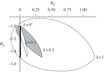
Figure 6. The convex sets Rl with l=0+, 0.1, 0.3 and 1 are shown. The set R0+ is the vertical segment with the endpoints (0,−0.9878. . .) and (0,−1.5).
Next, the intersection of the half-planes r,ei ≥ri is built. It is a convex polygon approximating the required set Rl, and the approximation accuracy
increases as n increases. The value n=100 was used in our calculations.
In figure 6, the sets Rl are shown for l=0+, 0.1, 0.3 and 1. The set R0+ is the vertical segment {0} × [−1.5, −0.9878], R0.1 is the thin set with white interior and R0.3 is the set with grey interior. The largest set is R1.
Infigure 7, the same sets are shown in more detail. Infigure 7b–d, additionally, we present the regions corresponding to all possible kinds of roughness related to triangular cavities (and to cavities formed by combinations of different triangles), with the angles being multiples of 5◦. These regions are coloured grey. Forl=0+, the corresponding region is the vertical interval {0} × [−1.42, −1] marked by a (slightly shifted) dashed line in figure 7a.
The part of the set Rl situated to the left of the vertical axis corresponds to resistance forces producing the proper Magnus effect. The part of Rl to the right of this axis is related to forces that cause the inverse Magnus effect. We can see that the majority of the set (in the case l=1, approx. 93.6% of the area) is situated to the right of the axis. This suggests that the inverse effect is a more common phenomenon than the proper one. Actually, although theorem 2.2 guarantees the existence of an everywhere dense subset ofRl generated by shapes of roughness, we never encountered a shape producing the proper Magnus effect (and thus corresponding to a point on the left of the vertical axis).
(b)Special cases of rough discs
We present here only the final expressions for the forces and their moments calculated by formula (2.13)–(2.20) from theorem 2.3; the calculation details are omitted.
(1) Circle (no cavities). The measure n0 corresponding to the circle is given by
dn0(x,y)=cosx ·d(x +y). One has RT[n0,l] =RI[n0,l] =0 and RL[n0,l] = −1.
–1.5 –1.4 –1.3 –1.2 –1.1 –1.0 –1.0
–1.1
–1.2
–1.3
–1.4
–1.5
–1.0
–1.2
–1.4
–1.6 0
0 –0.5
(a) (b)
(c) (d)
–1.0 0.5 1.0
0 0.25 0.50 0.75 1.00 0.1
RL
–1.0
–1.1
–1.2
–1.3
–1.4
–1.5 RL
RL
RL
RT RT
RT RT
0.2 0.3
0 0.1 –0.1
–0.2 0.2
Figure 7. The sets Rl with (a) l=0+, (b) 0.1, (c) 0.3 and (d) 1 are shown here separately. The valuesR[n,l], with n=n0,n,nrect,n▽,n⊗ are indicated by the symbols open circle, filled diamond,
open square, inverse triangle and circumscribed cross, respectively. (a) The region generated by triangular cavities is marked by a (slightly shifted) vertical dashed line. It is the interval with the endpoints (0,−1) and (0,−1.42). (b–d) The regions generated by triangular cavities are painted over.
(2) Retroreflector. There exists a unique measure n∈Psymm supported on
the diagonal x =y; its density equals dn(x,y)=cosx ·d(x −y). We believe that
there is no cavity generating this measure; however, according to theorem 2.2, there do exist cavities approximating it; that is, there exists a sequence of rough discs B3 such that nB3 weakly converge to n (see Plakhov & Gouveia (2007)
for an explicit construction). One has RT[n,l] =3pl/8, RL[n,l] = −3/2 and RI[n,l] = −3l/2. Thus, the longitudinal component of the resistance force does not depend on the angular velocity l, while the transversal component and the moment of this force are proportional to l.
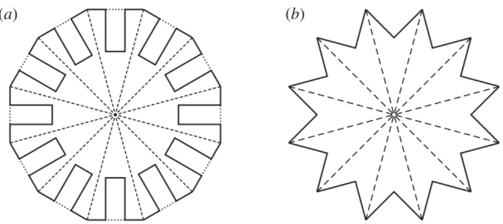
(a) (b)
Figure 8. (a) A rough disc with rectangular cavities. (b) A rough disc with triangular cavities.
height (width)/(height of the rectangle)=3. A smaller side of each rectangle is contained in a side of the polygon, besides |side of the rectangle|/|side of the polygon| =1−3. Then nB=nrect+o(1), where nrect=(n0+n)/2 and o(1) stands
for a measure weakly converging to zero as 3→0+. One can easily calculate that
RT[nrect,l] =3pl/16, RL[nrect,l] = −1.25 and RI[nrect,l] = −3l/4.
(4) Triangular cavity. The sets Bm representing the rough disc B are regular m-gons with m right isosceles triangles taken away (figure 8b). Then the measure nB =:n▽ has the following support (which looks like an inclined letter H): {x +y= −p/2 :x ∈ [−p/2, 0]} ∪ {y=x:x ∈ [−p/4,p/4]} ∪ {x +y=p/2 :x ∈ [0,p/2]}. The density of this measure equals dn▽(x,y)=cosx · (c[−p/2,−p/4](x)d(x +y+p/2) + c[−p/4,p/4](x)·d(x −y) + c[p/4,p/2](x)d(x +y−
p/2))+ |sinx| ·(c[−p/4,0](x)d(x +y+p/2) − c[−p/4,p/4](x)d(x −y)+c[0,p/4](x)d (x +y−p/2)). One has R[n▽, 0+] =(0;−√2)T and RI[n▽, 0+] =0; R[n▽, 1] = (1/4+3p/16; 3p/16−2)T. The rest of the values are still unknown.
(5) Cavity realizing the product measure. Consider the measure n⊗ with the density dn⊗(x,y)=(1/2) cosxcosydx dy. Evidently, in this case,n⊗∈Psymm. The
angles of incidence and of reflection are statistically independent; so to speak, at the moment when the particle leaves the cavity, it completely ‘forgets’ its initial velocity. Here we have RT[n⊗,l] =(10l+l3)p/80 for 0<l≤1; RL[n⊗, 1] = −3/4−p/5≈ −1.378 and RI[n⊗,l] = −3l/4 for any l. The remaining values are unknown.
The points in figure 7a–d corresponding to cases 1–5 are indicated by special symbols: n0 is marked by a circle, n is marked by a diamond; nrect, by an open
square; n▽, by a triangle and n⊗, by a circumscribed cross.
4. Dynamics of a rough disc
The motion of the spinning rough disc B is determined by the values RT[nB,l], RL[nB,l]andRI[nB,l]. For the sake of brevity, below we omit the fixed argument
Using equations (2.9) and (2.10), one rewrites the equations of motion (1.1) and (1.2) in the form
dv
dt =
8rrv2
3M RL(l), (4.1)
dq dt = −
8rrv
3M RT(l) (4.2)
and d(lv)
dt =
8r3rv2
3I lRI(l). (4.3)
Recall that b=Mr2/I is the inverse relative moment of inertia. The special values that b can take are: b=1, when the mass is concentrated near the disc boundary, and b=2, when the mass is uniformly distributed inside the disc. In the intermediate case, when the mass is arbitrarily (generally speaking, non-uniformly) distributed inside the disc, it holds b≥1.
With the change of variables dt=(8rrv/3M) dt, equations (4.1)–(4.3) are transformed into the following ones:
dl
dt =bRI(l)−lRL(l), (4.4)
dv
dt =vRL(l) (4.5)
and dq
dt = −RT(l). (4.6)
Denote bys the path length of the disc; thus, ds/dt=v. One readily finds that s is proportional to t, s=(3M/8rr)t.
Below, we solve the system of equations (4.4)–(4.6) for cases 1–3 considered in §3b. Next, we determine the dynamics numerically for some kinds of triangular cavities. A more detailed study of dynamics in the general case will be addressed elsewhere.
(1) Circle. One has dl/dt= −l, dv/dt= −v and dq/dt=0; therefore the circle moves straightforward. Solving these equations, one obtains that its centre moves according to the equation x(t)=(3M/8rr) ln(t−t0)e+x0, where t0∈R, e∈S1 and x0∈R2 are constants. Thus, having started the motion at some moment, the circle passes a half-line during infinite time. This equation also implies that the motion cannot be extended to all t∈R.
(2) Retroreflector. Here the system (4.4)–(4.6) takes the form dl
dt = −
3l(b−1)
2 ,
dv
dt = − 3v
2 and dq dt = −
3pl
8 . (4.7)
0 4
(a) (b)
3
1.5
1.0
0.5 2
1
1 2 3 4 5
(ii) 60°, 60°, 60°
(ii) 60°, 60°, 60°
(i) 30°, 120°, 30°
g(l) a(l)
(i) 30°, 120°, 30°
6 7 8 0 1 2 3 4 5 6 7 8
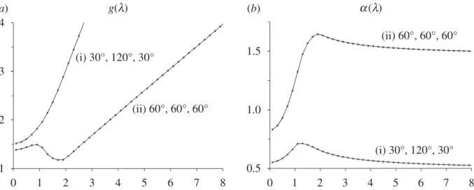
Figure 9. The functions (a) g(l)=lRL(l)/RI(l) and (b) a(l)=4RT(l)/l are shown for the
triangular cavities with the angles (i) 30◦, 120◦, 30◦ and (ii) 60◦, 60◦, 60◦.
In the case b>1, we have s(t)=(M/4rr) ln(t−t0), q=q0+const.· exp(−(b−1)(4rr/M)s) andl=(4/p)(b−1)(q−q0). The path length once again depends logarithmically on the time, the relative angular velocity l converges to zero and the direction q converges to a limiting value q0; thus, the values l and q are exponentially decreasing functions of the path length and are inversely proportional to the (b−1)th degree of the time passed since a fixed moment. The trajectory of motion is a semibounded curve approaching an asymptote as t→ +∞.
(3) Rectangular cavity. Equations of motion (4.4)–(4.6) in this case take the form dl/dt= −3l(b−5/3)/4, dv/dt= −5v/4 and dq/dt= −3pl/16. Solving these equations, one obtains t=(4/5) ln(t−t0), v=v0e−5t/4, l= l0e3t(5/3−b)/4 and q=q0+(pl0/4(b−5/3)) e3t(5/3−b)/4. Thus, the path depends on t logarithmically, and the relative angular velocity and the rotation angle are proportional to (t −t0)1−3b/5 and to exp((2rr(5−3b)/3M)s).
If b<5/3, then l and q tend to infinity, and the trajectory of the disc centre is a converging spiral. In the case b>5/3, l converges to zero, q converges to a constant value and the trajectory is a semibounded curve approaching an asymptote as t→ +∞. In the case b=5/3, l is constant, and the trajectory is a circumference of radius 2M/(prrl).
Finally, we examine numerically some triangular cavities. It is helpful to denote g(l)=lRL(l)/RI(l) and rewrite equation (4.4) in the form
dl
dt = −RI(l)(g(l)−b). (4.8)
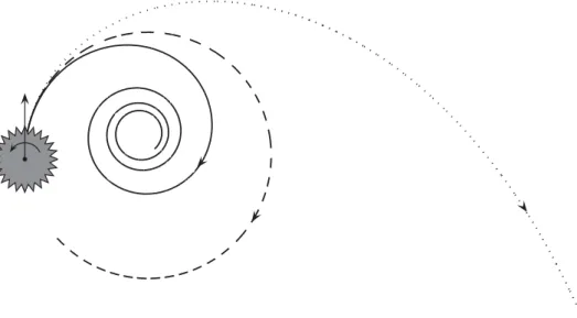
Figure 10. Three kinds of asymptotic behaviour of a rough disc with roughness formed by equilateral triangles and with 1.38<b<1.49: (I) converging spiral (solid line); (II) circumference (dashed line); (III) curve approaching a straight line (dotted line).
The disc behaviour is richer in case (ii) of the equilateral triangle. If 1.38<b<
1.49, then three kinds of asymptotic behaviour may be realized, depending on the initial conditions: (I) the trajectory is a converging spiral, (II) the trajectory approaches a circumference, and (III) the trajectory approaches a straight line (figure 10). If 1.16<b<1.38, only two asymptotic behaviours of types (I) and (II) are possible; if b>1.49, then the possible behaviours are (I) and (III); and if b<1.16, the asymptotic behaviour is always (I).
In the case of triangular cavities, as our numerical evidence shows, the function g(l) monotonically increases for l sufficiently large and liml→+∞g(l)= +∞. This implies that the trajectory is a converging spiral for appropriate initial conditions (namely, if the initial angular velocity is large enough). If, besides,
b is large enough (that is, the mass of the disc is concentrated near the centre), the trajectory may also be a curve approaching a straight line. If the function g has intervals of monotone decrease (as for the case of the equilateral triangle), then the trajectory may also approach a circumference. The length of the disc path is always proportional to the logarithm of time.
5. Conclusions and comparison with the previous works
In our opinion, the inverse Magnus effect in highly rarefied media is caused by two factors:
(i) Non-elastic interaction of particles with the body. A part of the tangential component of the particles’ momentum is transmitted to the body, resulting in creation of a transversal force.
In the papers by Borg et al. (2003), Ivanov & Yanshin (1980), Wang (1972) and Weidman & Herczynski (2004), the impact of factor (i) is studied. Moreover, the body is supposed to be convex and therefore factor (ii) is excluded from the consideration. In these papers, the force acting on a spinning body moving through a rarefied gas is calculated, and, additionally, the moment of this force slowing down the body’s rotation is determined (Ivanov & Yanshin 1980). The following shapes have been considered: a sphere, a cylinder (Ivanov & Yanshin 1980; Weidman & Herczynski 2004), convex bodies of revolution (Ivanov & Yanshin 1980) and right parallelepipeds of regular polygon section (Weidman & Herczynski 2004). The interaction of the gas particles with the body is as follows: a fraction 1−at of the incident particles is elastically reflected according to the rule ‘the angle of incidence is equal to the angle of reflection’, while the remaining fraction at of the particles reaches thermal equilibrium with the body’s surface, and is reflected as a Maxwellian (Wang 1972; Ivanov & Yanshin 1980; Borg et al. 2003). In the paper byWeidman & Herczynski (2004), a somewhat different model of interaction is considered, where the reflected particles acquire a fraction at of tangential momentum of the rotating body. The transversal force results from the tangential friction and acts on the body in the direction associated with the inverse Magnus effect. It is remarkable that for different models and different shapes of the body, the formula for the transversal force is basically the same. If the rotation axis is perpendicular to the direction of the body’s motion, then this force equals
1
2atMguv, (5.1)
where Mg is the mass of the gas displaced by the body, u is the angular velocity of the body and v is its translation velocity. (Note that inBorg et al. (2003), this formula appears in the limit of infinite heat conductivity or zero gas temperature.) Weidman & Herczynski (2004) found that for parallelepipeds of regular n-gon section with n odd, the transversal force depends on time, and the value of this force was determined. It is easy to calculate, however, that the time-averaged force is equal to equation (5.1).
In the present paper, in contrast, we concentrate on the study of factor (ii). We suppose that all collisions of particles with the body are perfectly elastic (that is, at=0), and therefore there is no tangential friction. We restrict ourselves to the two-dimensional case and suppose that the body is a disc with small cavities on its boundary, or a rough disc. The Magnus effect is due to multiple reflections of particles in the cavities. We study here all logically possible cases of cavities. According to equation (2.9), the transversal force equals
1
2a(l)Mguv,
where l=ur/v, Mg =pr2r is the total mass of gas particles displaced by the body, a(l)=a(l,n)=(16/3p)RT[n,l]/l and n is the measure characterizing the shape of the cavities. The function a depends on both n and l. In particular, a
are shown in figure 9b. We see that this function significantly depends on the velocity of rotation l; in general, the variation of a(l) with n fixed can be more than twofold.
We conclude that the impact of both factors (i) and (ii) is unidirectional, and so they strengthen each other. Moreover, the formulas for the transversal force are similar; one should just substitute the function a(l,n) for at. We have seen that a(l,n) can be significantly greater than 1, while at≤1. This can be just an artefact of our model being two-dimensional.
In a forthcoming work, we are planning to extend our consideration to the three-dimensional case and to media with a positive temperature. This seems to be more or less straightforward. A more challenging task would be studying the joint impact of non-elastic multiple collisions in the cavities. Also, it would be very interesting to study the effect in ‘not so rarefied’ media and find the critical value of density corresponding to reversal of the Magnus effect.
Apart from its physical meaning, studying the dynamics of a spinning rough disc (or, more generally, of a non-circular body) in a rarefied medium represents a nice mathematical problem, which originates in classical mechanics and has close connection with Newton’s aerodynamic problem (Newton 1687). According to our numerical simulations, the most part of all possible roughnesses (93.6% for l=1) correspond to the inverse Magnus effect, and only a small portion of them corresponds to the proper one. We know that roughnesses corresponding to the proper Magnus effect do exist, but have no idea how they should look and not one of such roughnesses has been found. Another interesting question concerns the description of admissible trajectories and is closely related to the associated problem of (vector-valued) Monge–Kantorovich OMT. In particular, the existence, in the same body, of a roughness corresponding to the proper Magnus effect for some values of l and to the inverse one for others would imply the existence of a rough disc with a strange zigzag trajectory.
This work was supported by the Centre for Research on Optimization and Control (CEOC) from the ‘Fundação para a Ciência e a Tecnologia’ (FCT), cofinanced by the European Community Fund FEDER/POCTI and by FCT: research project PTDC/MAT/72840/2006.
The authors are grateful to John Gough for useful comments on the text and to Gennady Mishuris for help in drawingfigure 10.
References
Borg, K. I. & Söderholm, L. H. 2008 Orbital effects of the Magnus force on a spinning spherical satellite in a rarefied atmosphere.Eur. J. Mech. B/Fluids 27, 623–631. (doi:10.1016/ j.euromechflu.2007.11.001)
Borg, K. I., Söderholm, L. H. & Essénm, H. 2003 Force on a spinning sphere moving in a rarefied gas. Phys. Fluids 15, 736–741. (doi:10.1063/1.1541026)
Ivanov, S. G. & Yanshin, A. M. 1980 Forces and moments acting on bodies rotating around a symmetry axis in a free molecular flow. Fluid Dyn. 15, 449. (doi:10.1007/BF01089985)
Mehta, R. D. 1985 Aerodynamics of sport balls.Annu. Rev. Fluid Mech.17, 151–189. (doi:10.1146/ annurev.fl.17.010185.001055)
Newton, I. 1687Philosophiae naturalis principia mathematica. London, UK: Streater.
Plakhov, A. 2009a Billiards and two-dimensional problems of optimal resistance. Arch. Ration. Mech. Anal.194, 349–382. (doi:10.1007/s00205-008-0137-1)
Plakhov, A. 2009b Billiard scattering on rough sets: two-dimensional case. SIAM J. Math. Anal. 40, 2155–2178. (doi:10.1137/070709700)
Plakhov, A. & Gouveia, P. 2007 Problems of maximal mean resistance on the plane.Nonlinearity 20, 2271–2287. (doi:10.1088/0951-7715/20/9/013)
Plakhov, A. & Tchemisova, T. 2009 Force acting on a spinning rough disk in a flow of non-interacting particles.Dokl. Math.79, 132–135. (doi:10.1134/S1064562409010396)
Prandtl, L. 1926 Application of the ‘Magnus Effect’ to the wind propulsion of ships.Die. Naturwiss. 13, 93–108 [NACA-TM-367].
Rachev, S. T. & Rüschendorf, L. 1998 Mass transportation problems. Vol. 1: Theory. Vol. II: Applications. Probability and its Applications (New York), xxvi+508pp. New York, NY: Springer-Verlag.
Rubinov, S. I. & Keller, J. B. 1961 The transverse force on a spinning sphere moving in a viscous fluid.J. Fluid Mech. 11, 447–459. (doi:10.1017/S0022112061000640)
Villani, C. 2003 Topics in optimal transportation. Graduate Studies in Mathematics, no. 58, xvi+370pp. Providence, RI: American Mathematical Society.
Wang, C.-T. 1972 Free molecular flow over a rotating sphere. AIAA J. 10, 713. (doi:10.2514/ 3.50192)


![Figure 5. The ‘level sets’ R 1,c = { all possible values of R [ n, 1 ] , with R I [ n, 1 ] = c } are shown for 21 values of c, from left to right: c = 0, − 0.075, − 0.15, − 0.225,](https://thumb-eu.123doks.com/thumbv2/123dok_br/16978414.762704/14.892.107.776.102.337/figure-level-sets-possible-values-shown-values-right.webp)