Experimental Study of the Performance of a Low Consumption Electric Car Prototype

UNIVERSIDADE DA BEIRA INTERIOR

Engenharia

Experimental Study of the Performance of a Low

Consumption Electric Car Prototype

Alexandre Manuel Domingues Correia

Dissertação para obtenção do Grau de Mestre em

Engenharia Aeronáutica

(Ciclo de estudos integrado)

(Versão corrigida após defesa)

Orientador: Professor Doutor Miguel Ângelo Rodrigues Silvestre

"Tudo é ousado para quem nada se atreve."

Aknowledgments

Firstly I thank my advisor Miguel Ângelo Rodrigues Silvestre for giving me the opportunity of developing my dissertation for master’s degree in a thematic that is my passion since my childhood and for the time he dedicated to me and to this study.

Thanks to Professor Pedro Gabriel F. L. B. Almeida for the aid in the topographic measurements and for providing all the material necessary.

I also have to thank my teammates of the AERO@Ubi, for all the time spent with the prototype. Without their dedication, this study could not be achieved.

To my friends and to new friendships, for being my company and support.

Resumo

Nesta dissertação são descritas todas as medidas para a caracterização do desempenho de um veículo terrestre protótipo elétrico de alta eficiência energética. A equipa AERO@Ubi da Universidade da Beira Interior, Covilhã, desenvolveu um veículo que competiu nas edições 2014 e 2015 da Shell Eco-Marathon®, que teve lugar em Roterdão. A equipa apresentou-se com um protótipo que se destaca em diversos métodos inovadores de movimento e design. Entre estas inovações estão presentes um corpo aerodinâmico distinto, que difere da forma convencional de gota de água, a utilização de um método de viragem que consiste na inclinação do protótipo com apenas uma roda na frente e o uso de pneus radiais bem como rolamentos de cerâmica. O protótipo foi submetido a vários testes de forma a caracterizar o coeficiente de arrasto aerodinâmico e o coeficiente de atrito de rolamento a fim de quantificar as perdas relacionadas a atritos. Estes testes serão descritos em pormenor no capítulo 3 e podem ser divididos em três fases: a fase preliminar, que incluiu medições topográficas de corredores e respetivas rampas de lançamento na Faculdade de Engenharia da Universidade da Beira Interior, bem como estradas com diferentes inclinações no Parque Industrial do Tortosendo; uma fase inicial, em que os componentes do carro foram testados separadamente, sem ou com mínima influência de outros componentes ou condições meteorológicas; uma fase final, em que o protótipo foi testado como um todo, através de descidas de estradas, a fim de verificar as diferentes velocidades terminais atingidas para diferentes inclinações de estradas. Os resultados são analisados e comparados com os resultados obtidos noutros estudos. Na fase inicial, os resultados foram encorajadores com o protótipo atingindo um valor de coeficiente de atrito de rolamento de 0,002 levando a um total previsto de 2 N de força de atrito de rolamento para 1000 N de peso do protótipo com piloto. Na fase final do teste, as perdas aumentaram significativamente para os 9 N o que indica uma característica não identificada do protótipo. O protótipo obteve um resultado de 331 km/kW.h, alcançando o 19º lugar para protótipos com propulsão a bateria elétrica na Shell Eco-Marathon® Europa.

Palavras-chave

Shell Eco-Maratona®; Coeficiente de Arrasto Aerodinâmico; Coeficiente de Atrito de Rolamento; Velocidade Terminal.

Resumo Alargado

Atualmente verifica-se a necessidade de reduzir as emissões de gases produtores de efeito de estufa, bem como um menor consumo de combustíveis fósseis (também estes libertadores de gases de efeito de estufa), de modo a contrariarmos a tendência dum futuro insustentável. Para isso a Shell promove a Shell Eco-Maratona® com o intuito de sensibilizar futuros engenheiros para esta temática, levando ao desenvolvimento de conceitos e protótipos de alta eficiência energética. A equipa AERO@Ubi da Universidade da Beira Interior, da Covilhã, desenvolveu um protótipo de elevada eficiência energética com propulsão elétrica, que competiu nas edições 2014 e 2015 da SEM®, realizadas em Roterdão. A equipa apresentou um protótipo que se destaca em diversos aspetos, por apresentar métodos inovadores de locomoção e conceção. Entre eles inclui-se: um corpo aerodinâmico que se distingue da convencional forma de gota de água; um método de viragem que consiste na inclinação do protótipo e com apenas uma roda na frente; na utilização de pneus radiais e rolamentos cerâmicos.

Nesta dissertação começa-se por descrever o protótipo desenvolvido e suas características bem como uma revisão bibliográfica e discussão de trabalhos previamente realizados por outros investigadores, ao qual, os resultados obtidos neste estudo foram comparados com os conseguidos por outros autores de modo a validar as diferentes metodologias e testes práticos usados pelas equipas que competiram em diferentes edições da SEM®. Posteriormente, fez-se uma descrição dos testes a que o protótipo foi sujeito com o propósito de caracterizar o coeficiente de arrasto aerodinâmico e o coeficiente de atrito de rolamento por quantificação das perdas. Estes testes foram divididos em três fases: uma pré-fase, onde foram feitos levantamentos topográficos do corredor e respetiva rampa de lançamento, na Faculdade de Engenharia da Universidade da Beira Interior, para testes iniciais, e em estradas, com diferentes declives, do Parque Industrial do Tortosendo, para realização de testes num estado mais avançado do protótipo; uma fase inicial, onde foram testados componentes do carro de uma forma isolada, sem qualquer ou com a mínima influência de outros componentes ou de condições climatéricas; uma fase final, onde o protótipo foi testado como um todo, através de descidas em estradas, onde são atingidas diferentes velocidades terminais para diferentes declives. Por último, no capítulo 4, são apresentados os resultados obtidos com recurso a gráficos.

Inicialmente o protótipo apresenta bons resultados, que, com base nos testes da fase inicial, previam uma força total de resistência ao movimento, isto é a força de atrito de rolamento e força de atrito aerodinâmico, de 4 N. Contudo, este quadro não se verificou numa situação real, pois quando testado nas descidas de diferentes rampas do Parque Industrial do Tortosendo, os valores de força dissipada dispararam para a casa dos 9N, que foi, igualmente, o que aconteceu na edição de 2015 da SEM®.

No início deste trabalho, não foram consideradas perdas mecânicas estruturais do carro, por se considerar que eram perdas extremamente baixas para uma perspetiva macroscópica. No entanto, esta grande discrepância de valores pode ter origem em erros na construção da estrutura e carroceria, que originam fricções e conflitos entre os diversos componentes. O protótipo teve o melhor resultado de 331km/kwh na edição de 2015 da SEM®, arrecadando o 19º lugar na tabela Europeia de protótipos com propulsão a baterias elétricas.

Palavras-chave

Shell Eco-Maratona®; Coeficiente de Arrasto Aerodinâmico; Coeficiente de Atrito de Rolamento; Velocidade Terminal.

Abstract

In this dissertation all steps to characterize the performance of an electric prototype road vehicle of high energy-efficiency are portrayed.

The AERO@Ubi team from the University of Beira Interior, Covilhã, developed a vehicle that competed in the 2014 and 2015 editions of the Shell Eco-Marathon®, which took place in Rotterdam. The team presented a prototype that stands out for its innovative methods of movement and design. Among these innovations is a distinguished aerodynamic body, that differs from the conventional form of water drop, and instead uses a turning that consists in tilting the prototype with only one wheel at the front and employs radial tires as well as ceramic bearings.

The prototype was subjected to several tests in order to characterize the aerodynamic drag coefficient, the rolling friction coefficient and the lift coefficient in order to quantify the losses related to friction and aerodynamic drags.These tests, which will be described in detail in Chapter 3 can be divided into three stages: a preliminary stage, which included topographic measurements of corridors and respective launch ramps at the Faculty of Engineering of the University of Beira Interior as well as of roads with different slopes at Tortosendo Industrial Park were carried out; an initial stage, where the car components were tested separately , without or with minimal influence from other components or weather conditions; a final stage, where the prototype was tested, as a whole, through downhill roads in order to verify different terminal velocities down different slopes.

The results are analyzed and compared with results obtained in other studies. In the initial stage the results were encouraging as the prototype revealed a rolling friction coefficient value of 0.002 leading to a foreseen total of 2 N of rolling friction force for a 1000 N of the prototype with the pilot weight. In the final stage of testing, the results increase significantly to 9 N and this may suggest an unidentified feature of the prototype.

The prototype obtained a result of 331 km/kWh, reaching the 19th _{place for prototypes with electric battery}

in the Shell Eco-Marathon® Europe.

Contents

Chapter 1Introduction 1

1.1 The Shell Eco-Marathon® 2

1.2 Summary 3

1.3 Objectives 3

Chapter 2 Literature Review 5

2.1 Vehicle Efficiency: Basic Theory 5

2.1.1 Dissipative Forces 5

2.1.1.1 Rolling Friction 6

2.1.1.2 Drag 8

2.1.1.3 Bearing Losses 10

2.1.2 Newton’s First Law and Conservation of Energy 11

2.1.2.1 Acting Forces in a Slope 12

2.2 Vehicle Components 13

2.2.1 Tires 13

2.2.2 Tire’s Inflation Pressure 14

2.2.3 Bearings 15

2.2.4 Toe Angle 15

2.2.5 Camber Angle 16

2.2.6 Cornering Drag 17

2.2.7 Ground Clearance 18

2.3 State of the Art 18

Chapter 3 Methodology 21 3.1 Vehicle Description 21 3.1.1 Car Specifications 22 3.1.2 Wheels 23 3.1.2.1 Tires 23 3.1.2.2 Bearings 24 3.1.3 Steering Gear 25

3.1.4 Body Shape 27

3.1.5 Propulsion System 28

3.2 Experiments Performed 28

3.2.1 Wheel’s Bearing Losses Measurement 29 3.2.2 Ramp and Horizontal Coasting Test 31 3.2.3 Horizontal Road Dissipative Force Measurements 32

3.2.3.1 Dynamometer 33

3.2.4 Slope Terminal velocities Tests 34

3.3 Test Roads 37

3.3.1 Topographic Characterization Study 37 3.3.1.1 Horizontal Corridor Road and Launch Ramp 38 3.3.1.2 Tortosendo Industrial Park Roads 40

Chapter 4 Results 47

4.1 Wheel’s Bearing Losses Measurements Results 47 4.2 Car Coasting Rolling Friction Tests Results 49 4.3 Flat Road Rolling Friction Force Measurements Results 52 4.4 Slope Terminal velocities Tests Results 54

4.5 SEM® Result Analysis 56

4.6 Uncertain Analysis 57 Chapter 5 Conclusion 59 5.1 Future Work 59 Chapter 6 Bibliography 61 Chapter 7 Appendix 63 7.1 Matlab Codes 63 7.2 Images 65

List of Figures

Figure 1.1- CO2 Concentration in the atmosphere from 650,000 years ago till the present [1]. 1 Figure 1.2 - Track plan of SEM® at Rotterdam. 2 Figure 2.1 - Dynamic forces acting on a vehicle in function of velocity, resulting in a total

force [10]. 6

Figure 2.2 - Physical causes of rolling friction, [6]. 7 Figure 2.3 - Scheme of attached and separated streamline flow [4]. 10 Figure 2.4 - Example of bearing constituents. 11 Figure 2.5 - Acting forces on a body in a slope. 13 Figure 2.6 - Inflation pressure influence on the rolling friction coefficient on tires 45-75R16

[4]. 14

Figure 2.7 - Toe angle influence in tire drag by PAC-Car II [4]. 16 Figure 2.8 - Negative camber angle influence on rolling friction coefficient,[4]. 17 Figure 2.9 - Wheel cornering and sideslip angle. 17 Figure 2.10 - Minimal drag height of ground clearence for smaller interference drag [10]. 18 Figure 2.11- Drag coefficient with car's body development [16]. 19 Figure 3.1 - Different stages of the prototype's body construction. 21 Figure 3.2 – Michelin radial tires 45-75R16 (left) and Michelin tires 44-406 (right). 24 Figure 3.3 - Ceramic and metallic bearings used in the prototype. 25 Figure 3.4 – Prototype’s tilting turning. 26 Figure 3.5 - Representation of toe angle tuning mechanism. 26 Figure 3.6 - 3 D Cartesian coordinate system applied to the prototype. 27 Figure 3.7 – Propulsion system, controller and motor. 28 Figure 3.8 – Wheel’s bearing losses measurement scheme. 29 Figure 3.9 - Car coasting rolling friction test scheme. 31 Figure 3.10- Dynamometer and elastic rubber band used in the rolling friction force

measurements test. 33

Figure 3.11 - Passengers vehicle used to validate slope terminal velocities equations for 2

ramps. 36

Figure 3.12 - Results obtained by passenger vehicle terminal velocities slopes test. 37 Figure 3.13 - Equipment used for topographic measurements. 38 Figure 3.14 - Flat road topographical measurement. 39 Figure 3.15 - Launching ramp topographical measurements. 39 Figure 3.16 – Map of the streets used in Tortosendo Industrial Park roads test. 40 Figure 3.17 - Street Parkurbis 1 sector a topographic measurements. 41 Figure 3.18 - Street Parkurbis 1 sector b topographic measurements. 41

Figure 3.19 - Street Parkurbis 2 sector a topographic measurements. 42 Figure 3.20 - Street Parkurbis 2 sector b topographic measurements. 42 Figure 3.21 - Street Parkurbis 3 topographic measurements. 43 Figure 3.22 - Street I topographic measurements. 43 Figure 3.23 - Street B sector a topographic measurements. 44 Figure 3.24 -Street B sector b topographic measurements. 44 Figure 3.25 - Street C topographic measurements. 45 Figure 4.1 – Bearing torque and wheel's inertia of right back wheel. 48 Figure 4.2 – Bearing torque and wheel's inertia of left back wheel. 48 Figure 4.3 - Toe angle influence on the distance reached from a launching ramp of 1 m. 49 Figure 4.4 - Toe angle influence on the distance reached from a launching ramp of 1.8 m. 50 Figure 4.5 - Variation of rolling friction coefficient with wheel's toe angle. 51 Figure 4.6 – Towing test force variation along the road. 53 Figure 4.7 - Dissipative force variation with terminal velocity. 54 Figure 4.8 - Terminal velocity for different slopes. 55 Figure 4.9 - Terminal velocity for different slopes compared with theoretical values. 55

List of Tables

Table 3.1 - Prototype specifications – dimensions and weights. 22 Table 3.2 – Prototype component's weights. 22 Table 3.3 - Steel and ceramic bearings' weight comparison, used by the prototype. 24 Table 3.4 - Aerodynamic specs comparison, [21]. 27 Table 3.5 – Dynamometer weights’ test. 33 Table 3.6 - Vehicle’s specifications by carfolio.com [28]. 36 Table 3.7 - Launching ramp characteristics. 39 Table 3.8 - Street Parkurbis 1 sector a characteristics. 41 Table 3.9 - Street Parkurbis 1 sector b characteristics. 41 Table 3.10 - Street Parkurbis 2 sector a characteristics. 42 Table 3.11 - Street Parkurbis 2 sector b characteristics. 42 Table 3.12 – Street Parkurbis 3 characteristics. 43 Table 3.13 - Street I characteristics. 43 Table 3.14 - Street B sector a characteristics. 44 Table 3.15 - Street B sector b characteristics. 44 Table 3.16 - Street C characteristics. 45 Table 4.1 - Average values obtained for the best tuning in the ramp and horizontal coasting

test. 52

Table 4.2 – Results obtained for towing force from ramp. 53 Table 4.3 - Results obtained for towing force heading ramp. 53 Table 4.4 - Error associated to devices used in primary measurements. 57 Table 4.5 – Uncertainty analysis of the results of the experimental tests. 58

List of Acronyms

DCA Aerospace Science Department AC Alternating Current

CNG Compressed Natural Gas

GTL Gas-to-Liquid

GW Global Warming

GHG Green-House Gases ppm Part per Million SEM® Shell Eco-Marathon®

Nomenclature

𝐹𝐷 Aerodynamic Draf Force, N

Ѳ𝑎 Angle Traveled During Wheel’s Acceleration, rad

Ѳ𝑏 Angle Traveled During Wheel’s Deceleration, rad

𝛼 Angular Acceleration, rad/s2

𝜔 Angular Velocity, rad/s 𝑄𝑏 Bearing’s Torque, N.m

𝐹𝑄_𝑏 Bearing’s Torque Force, N

δ Boundary Layer Thickness, m

CO2 Carbon Dioxide

CM Center of Mass

𝜌 Density of Air, kg/m3

𝐶𝐷 Drag Coefficient

𝐸𝑘𝑓 Final Kinetic Energy, N

𝑣𝑓 Final Velocity, m/s

𝑆𝑥 Frontal Area, m2

𝑔 Gravitational Acceleration, m/s2

𝐹𝑔 Gravitational Force, N

𝐹𝑔𝑥 Gravitational Force, in x-axis, N

𝐹𝑔𝑦 Gravitational Force, in y-axis, N

𝐸𝑝𝑖 Initial Potential Energy, N

𝑣 Kinetic Viscosity, Pa.s

𝐿 Length, m 𝐶𝐿 Lift Coefficient 𝑎 Linear Acceleration, m/s2 𝑣 Linear Velocity, m/s 𝑚 Mass, Kg CH4 Methane 𝐼 Moment of Inertia, Kgm2 𝐹𝑁 Normal Force, N O3 Ozone

𝛼 Pitch Angle, rad

𝑢∞ Relative Air Speed of Undisturbed Flow, m/s

𝐹𝑅 Resultant Force, N

𝑀𝑅 Resultant Moment, N.m

𝐶𝑟 or 𝜇𝑟 Rolling Friction Coefficient

𝑘𝑓 Rolling Friction Coefficient Dependent on the Velocity

𝑐𝑎and 𝑐𝑏 Rolling Friction Constants

𝐹𝑟 Rolling Friction Force, N

𝛥𝐼 Variation of Internal Energy, J 𝛥𝐾 Variation of Kinetic Energy, J 𝛥𝑈 Variation of Potential Energy, J 𝛥𝐸 Variation of Total Energy, J 𝑡𝑎 Wheel’s Acceleration Time, s

𝛼𝑤𝑏 Wheel’s Angular Braking (Deceleration), rad/s2

𝑡𝑏 Wheel’s Braking Time, s

ℎ𝑤 Weight’s Drop Height, m

𝑚𝑤 Weight’s Mass, Kg

𝐼𝑤 Wheel’s Moment of Inertia, Kg.m2

𝛽 Yaw Angle, rad

Hooke’s Law,

𝑘 Constant Factor Characteristic, N/m

𝛥𝑥0 Deformation, m

𝑥0 Length of Relaxed Position, m

𝐹 Restoring/reaction Force, N 𝐴0 Section Area, m2 𝜀 Specific Strain 𝜎 Stress Tensor, Pa 𝐸 Young’s Modulus Error Analysis,

𝛥𝑋 Device’s Error Measurement

D Difference on the value measured

𝑑 Square root of the sum of the squares of all the differences

q Uncertainty

Chapter 1

1 Introduction

Global warming is a much discussed and worrying theme nowadays. Scientists believe that the major cause of global warming (GW) is due to the concentration of greenhouse gases (GHG) in the atmosphere [1]. Among these GHG are included water vapor, responsible for 36-70% of the GW effects, carbon dioxide (CO2)

with 9-26% (commonly associated as the main GHG), methane, CH4, with 4-9% of greenhouse effect

influence, and ozone, O3, 3-7%.Human activities have since the start of the Great Industrial Revolution

(after the 1750s) been responsible for an abrupt increase of CO2 concentrations (36%) - from 280 ppm to

400 ppm in 2015 - and CH4 (148%) in the atmosphere, values which are far above those found in ancient ice

cores[2] (see Figure 1.1).

Between different human activities responsible for the increase of GHG, transportation accounts for about 14% the total CO2 emissions [2]. Almost all transportation relies on liquid fuels and road transportation has

an important share in CO2 emissions. Several actions to reduce the emission levels of GHG were taken,

these include energy conservation and energy efficiency and use of low-carbon technologies (renewable energy, nuclear energy, etc.). In this scenario, Shell created the Shell Eco-Marathon® competition.

1.1 The Shell Eco-Marathon®

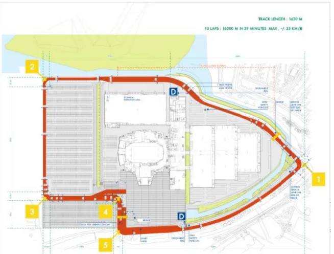
Combining the need to reduce emissions of GHG with the develop new means of propulsion without using fossil fuels or simply reducing emissions and optimizing transportation, Shell, with the annual Shell Eco-Marathon, SEM® competition events in different continents, aims to create a competition that challenges students and academics around the world to develop the most energy-efficient cars [3], both prototypes and urban concept vehicles with different sources of energy: electric, hydrogen, gasoline, diesel, alternative fuels (ethanol and gas-to-liquid, GTL) or compressed natural gas, CNG. The competition completed the 30th edition in 2015 and consisted in making 10 laps in an urban circuit represented in Figure 1.4, substantially flat, totaling approximately 16 km, within a maximum time of 39 minutes corresponding to an average speed of 25 km/h. The track has five 90ᵒ turns with a minimum inner turning radius of 9m, as seen in Figure 1.2. The track vertical profile and the turns characteristics present greatly affect the vehicles conception. Numerous factors influence the maximum range of the vehicle, and the driving strategy is one of them. One obvious strategy is, a maximum utilization of the available time and the achievement of smoother turns for the vehicle's efficiency optimization.

1.2 Summary

This document is divided in 5 chapters for a better comprehension of all the steps taken to conceive this study. An introduction is done, recalling the worldwide situation and the necessary attention to the consumption of fossil fuels along with the SEM® competition and the main objectives of this study. Following is a chapter where a bibliographic review on several ways of improving the performance of land vehicles and the state of the art englobing several experiments with different applications. The vehicle is descripted in the 3rd _{chapter, with its}

innovative characteristics, a detailed description of the tests the prototype was subjected and the previously made topographic measurements. The results are presented and discussed in the 4th _{chapter along with other obtained from different studies with the error analysis of the}

measurements made. The document finishes with the conclusion and future work necessary for a more complex prototype’s study with some images of the prototype and the competition annexed.

1.3 Objectives

Whatever type of vehicle energy source or propulsion, the ultimate goal is to optimize the efficiency in the energy conversion and minimize energy losses from the friction forces adverse to the movement of the car. Therefore, and departing from several projects previously developed, e.g. the vehicle’s prototype design and construction, this work has the following objectives:

 prototype characterization with concern to losses by friction, in particular, quantification of the rolling friction coefficient and drag area using various experimental techniques for the whole system or in separate components (i.e., each car component is tested with no or minimal influence from other components) to set the values of the various coefficients mentioned above;

 Identify any deviations from the expected theoretical design values;

Chapter 2

2 Literature Review

2.1 Vehicle Efficiency: Basic Theory

2.1.1 Dissipative Forces

Dissipative forces refers to all forces that oppose the free motion of a body leading to a deceleration and subsequent halting in the absence of a propulsion force. When it comes to losses for high efficiency land vehicle three types of losses can be found: aerodynamic drag, wheel bearing losses and wheel rolling friction.

According to Santin et al. [4], to maintain a highly energy-efficient vehicle in motion on a flat surface, both drag and wheel associated losses (rolling friction and bearing losses) are included (see Figure 2.1). However, Ed Burke [5] argues that for speeds slower than 13 km/h, wheel rolling and bearing frictions are accounted for 90% of the energy losses, knowing that drag increases the square with the gain of speed. Although this statement was made in a study on bicycle performance, where the front area is poorly distributed and not slim, we can consider that the value of the speed at which the drag can be considered negligible is slightly higher to the referred one, given the prototype’s surfaces aerodynamically optimized. This point is extremely important for a better analysis and discussion of the results obtained in the performance of the prototype tests, which will be described in the next chapter.

Figure 2.1 - Dynamic forces acting on a vehicle in function of velocity, resulting in a total force [10].

A detailed discussion of the whole physics associated to the previously types of losses mentioned above will follow using several schemes and data from other publications.

2.1.1.1 Rolling Friction

This force is intimately related to the normal force (vertical component of the contact force with the surface), in which the normal force component is opposite to the weight (product of mass and gravitational acceleration); Therefore the gravitational acceleration can be regarded as a constant value for various situations - the greater the mass of the moving object, the greater the normal force and consequently the greater resistance to movement. The rolling friction (or also called as rolling drag or rolling resistance) is originated mainly by wheel deformation, which is associated to the contact of a surface with the soft surface of the wheel, as seen in Figure 2.2.

Figure 2.2 - Physical causes of rolling friction, [6].

This contact between the wheel and the surface can be performed at several points (contact point), along a line (linear contact) or, more often, in an area (surface contact), although the first two relate to theoretical situations [7]. When there’s no wheel deformation and/or support surface, the contact between the surfaces will be point or linear (the theoretical contact type) at a point/line where no slip occurs. Having in mind that there is no slip, then the friction between the surfaces is a static friction. This static friction has a null resultant of work, which makes this friction a not dissipative force. This leads to the conclusion that the only opposing force to the movement, i.e., the only force that would cause any moving object to halt would be air resistance. However considering the non-stiffness and the deformation of surfaces, the contact will not be limited to a single point but to a deformed area. This will cause deformation, [7], commonly called rolling friction moment. So, rolling friction coefficient, or simply rolling friction, is the loss of energy in a horizontal plane, which will gradually decelerate the moving body, transforming the motion associated mechanical energy into thermal energy. The rolling friction is due to 3 physical causes: deformation of the wheel contact surface, drag caused by the wheel and micro-slipping between both surfaces. The viscoelastic properties of the tire constituent material leads to deformation while in contact with the solid surface, corresponding to about 90% [4] or between 80% and 95%, according to The Tyre: Rolling friction and Fuel Settings paper of Michelin [6], of the total energy losses, which is dissipated as heat, as the remainder percentage comes from losses of micro-slipping and drag caused by the rotation of the wheel.

The rolling friction coefficient, 𝐶𝑟, (or 𝜇𝑟 from other literary references) is a dimensionless value

obtained by dividing the rolling friction force, 𝐹𝑟, and normal weight component on the wheel, 𝐹𝑥:

Quoting Fuss [8], this coefficient can be used as a dependent and/or independent of speed according with to the velocity of the vehicle (see Figure 2.1). Starting with the independent of speed, we have:

𝐹𝑟= 𝐶𝑟 𝑚 𝑔 (2.2)

Where 𝑚 is the mass of the body and 𝑔 gravitational acceleration. Noting the above equation 2.2, isolating the rolling friction force, we get:

𝐹𝑟= 𝐶𝑟 𝐹𝑥 (2.3)

Therefore, we can assume that the normal component of the weight on the wheel is equal to the weight of component:

𝐹𝑥= 𝑚 𝑔 (2.4)

Linear dependence of velocity gives us:

𝐹𝑟= 𝑐𝑎+ 𝑐𝑏 𝑣 (2.5)

Where 𝑣 is velocity of the body and 𝑐𝑎 and 𝑐𝑏 friction coefficients.

Nonlinear dependence of velocity:

𝐹𝑟= 𝑐𝑎+ 𝑐𝑏 𝑣2 (2.6)

That can also be written in the following way:

𝐹𝑟= 𝐶𝑟 𝑚 𝑔 + 𝑘𝑓 𝑚 𝑔 𝑣2 (2.7)

Where 𝑘𝑓 is the rolling friction coefficient dependent on the velocity, 𝑣.

The rolling friction coefficient calculated from viscoelastic models behaves in a nonlinear way; because a tire is made of viscoelastic material with a non-linear behavior, then equations 2.6 and 2.7 are the most appropriate for this experimental study.

2.1.1.2 Drag

Drag is the force that opposes the motion of an object through the air. As discussed in the rolling friction, the same line of thinking can be taken to understand this type of energy loss. Aerodynamic drag is intimately related to the pressure distribution along the body and the more the streamlined flow is disturbed by the motion of the body, the higher the drag will be. We can think on this aerodynamic drag as a surface friction that depends on the properties of the flow and the body’s surface.

A smooth and waxed surface and a slender body will present a minor aerodynamic drag value than a blunt and rough body. The viscosity of the flow also changes the drag’s value.

We obtain the drag by the following expression: 𝐹𝐷 =

1

2 𝜌 𝑆𝑥 𝐶𝐷 𝑣2 (2.8)

Applying this equation to the prototype problem, density of the air, 𝜌, is a constant value during the race with a constant velocity, 𝑣, the frontal area of the prototype, 𝑆𝑥, and the dimensionless value of the drag

coefficient, 𝐶𝐷, are the most important factors in increased drag force. The product between 𝑆𝑥 and 𝐶𝐷 is

Note that 𝑆𝑥 changes depending on the pitch angle, 𝛼, and yaw angle, 𝛽, and to minimize the drag, the

equivalent flat plate area must be minimal too.

𝑆𝑥= 𝑆𝑥 ( 𝛼 , 𝛽 ) (2.9)

There are two main types of aerodynamic drags: surface friction drag and pressure drag.

Friction Drag

Due to the spread of air and condition of non-slipping fluid on the surface of a body, tangential stresses, τ, are created which are caused by the deceleration of the air. Dividing the fluid into streamlines, knowing that air velocity on the body surface is null, there are tangential stresses between each fluid streamline, so the streamlines will be decelerated by the other streamlines. At a certain distance relative air speed, 𝑢, will be 99% of 𝑢∞ (relative air speed of undisturbed flow). This distance is called the boundary layer, δ,

which increases along the surface of the body.

The value of the shearing stress varies with the type of flow in the boundary layer, which increases with the Reynolds, 𝑅𝑒. The Reynolds value is a dimensionless value that describes the flow behavior:

𝑅𝑒 =𝑢 𝐿

𝑣 (2.10)

Where 𝐿 is the length of the contact surface and 𝑣 the kinetic viscosity. The following values of Reynolds describe the flow behavior:

 0 < 𝑅𝑒 < 1 Highly viscous laminar flow

 1 < 𝑅𝑒 < 100 Laminar flow with great dependence of the Reynolds number

 100 < 𝑅𝑒 < 103 _{Laminar flow, respects the theory of boundary layer}

 103 _{< 𝑅𝑒 < 10}4 _{Transition flow}

 104 _{< 𝑅𝑒 < 10}6 _{Turbulent flow with dependence of Reynolds number}

 104 _{< 𝑅𝑒 < ∞ Turbulent flow}

Pressure Drag

This type of pressure is applied all around the body acting perpendicularly to the surface. It is possible to distinguish 4 types of pressure drag;

 Boundary Layer Thickness Drag – The increase of the boundary layer is directly related to the

potential flow and pressure field, in which an adverse pressure gradient can lead to a null relative speed causing the flow to separate from the surface and take the form of vortices. This flow separation causes increased drag, mainly pressure drag due to the pressure differential of front and rear surfaces along the surface [9].

subsequent reversal of the flow near the surface (see Figure 2.3). If the flow is not able to follow the body’s surface, then zone is created where the pressure is close to that of the separation point. The pressure at the separation point is usually lower than the ambient pressure and it is even lower if the separation point travels further forward on the body. For this reason, the further the reattachment of the flow to the body’s surface the longer the body is and its pressure will be minor. Blunt body shapes and airfoils with high angles of attack are examples of cases where flow separation occurs which significantly alters the distribution of pressure over the body and the aerodynamic drag characteristics.

Figure 2.3 - Scheme of attached and separated streamline flow [4].

 Induced Drag - Depending on the shape and angle of attack, any body into a flow produces lift

and downforce which cause induced drag. Unlike most land vehicles of high-speed, for high efficiency land vehicles moving at lower speeds, it is desirable that these forces have minimal influence on the movement. According to Tarnai G. [10] (as seen in PAC-Car II [4]) there are no improvements in rolling friction coefficient with the increase of lift forces.

 Interference Drag - The interference drag is due to the proximity of two distinct body

shapes emerged in the flow. When the pressure fields overlap there is a change in the characteristics of the flow. This may lead to an increase of the drag that results in an increase of the boundary layer displacement thickness. This increase may be due to a zone of increased flow velocity in the proximity of the bodies, such as the influence of the road in the aerodynamics of a road vehicle. A carefully design of the prototype’s body is important to reduce this type of drag. Equally important for that matter is the vehicle’s ground clearance.

Bearings have the main function of transmitting movement with the least friction possible, so it relies on the rolling mechanism itself (see Figure 2.4). This mechanism is far more efficient than sliding, however it still generates friction. Rolling bearings consist in low areas of contact with great loads concentration, leading to deformations. This high load may require bearing’s lubrication which lead to some losses by macro-sliding. Therefore, there are 4 types of energy losses [11]:

 Rolling Friction

- R

olling friction losses are associated with every rolling contacts. There are many losses related to the rolling friction namely the deformation of the rolling elements, which can cause micro slipping, and the adhesion forces between these elements and the inner and/or outer rings. There are also many energy losses in the introduction of a lubricant or during the excess rejection (elastohydrodynamic lubrication).

 Slipping Friction - Sliding is always present in rolling surfaces that can be divided in 2 types: Macro

slipping that is caused by the conformity because of more than one big geometry features and the micro slipping caused by the geometrical distortion and the elastic deformation.

 Seal Friction – It is caused by the occasional slippery provoked by great velocities and torques

generated by the seal and the moving counterface in contact.

 Drag Losses – These include the friction forces induced by the lubrication bath.

As it has been mentioned throughout this study, the prototype was subjected to various experimental tests to characterize its performance. However, for a better and more complete understanding of these methods, a brief introduction to some basic laws of physics, such as Newton's Laws and Energy Conservation is worth mentioning. Beginning with the Second Law of Newton, the principle of fundamental dynamics can be written as:

𝐹 = 𝑚 𝑎 (2.11)

𝑀 = 𝐼 𝛼 (2.12)

Where 𝐹 represents the resultant force acting on the body and 𝑀 is the resultant moment of the body's center of mass, CM, for a given mass, 𝑚, that inertia, 𝐼, for linear accelerations, 𝑎, or angular, 𝛼. However it is impossible to calculate the unknown quantities without the aid of additional relations between the linear speed and acceleration and angular speed and acceleration, such as friction force and normal force.

The principle of conservation of energy states that the amount of energy in a system remains constant. Transformations of energy type are possible, although its resultant force will remain the same. The energy change in a system can be described as follows:

𝛥𝐸 = 𝛥𝐾 + 𝛥𝑈 + 𝛥𝐼 (2.13)

Where ΔE represents the changes in the system’s total energy in the form of kinetic energy, potential and internal (frictional forces), respectively. The kinetic energy is the result of a quadratic function relating to speed, while the potential energy depends on the velocity.

𝛥𝐾 = 1

2 𝑚 𝛥𝑣2 (2.14) 𝛥𝑈 = 𝑚 𝑔 𝛥ℎ (2.15)

This law can be applied in certain cases, where small frictions or micro-slipping represent small decreases of mechanical energy, converting it into dissipated energy in the form of heat that can be neglected in a macroscopic perspective of the observer. This is the case of the losses of the wheel’s bearing experimental test where we can consider the system wheel/weight a closed system where there are no energy dissipated in the form of heat by frictions of the bearings and/or weight drop. While testing the prototype by coasting downhill slopes the same does not verify. Due to its large and complex system, the wheel’s CM translation, neither mechanical losses caused by friction of the components nor losses deriving from the tire’s micro-slipping are to be neglected. Hence, this must be considered as an open system where there are substantial exchanges of matter and energy, which must not be overlooked.

2.1.2.1 Acting Forces in a Slope

Considering that a horizontal plane a body in motion with null acceleration has three forces applied to its CM: gravitational force towards the center of the earth, normal force perpendicular to the contact surface and drag force, which is divided into aerodynamic drag and rolling friction drag with reverse direction of

abscises has the direction of the downward ramp and the gravitational force, due to the slope of the ramp, is divided in a y component (opposite to the positive direction of the y-axis) that is equal to the normal force, and a x component also with the direction of the downward ramp. See Figure 2.5:

Figure 2.5 - Acting forces on a body in a slope.

When the resultant force acting on the body is zero:

∑ 𝐹 = 𝐹𝐷+ 𝐹𝑟+ 𝐹𝑔𝑥= 0 (2.16)

It is reached a certain constant velocity when there’s no acceleration or deceleration; this velocity is called the terminal velocity. The gravitational force on the y-component is countered by the normal force, and the x component of gravitational force gives motion to the descending body. The terminal velocity reached is directly dependent on the body’s weight and on the slope of the ramp, the higher these are, the higher the velocity reached.

2.2 Vehicle Components

2.2.1 Tires

A common tire consists in two elements [4], rubber involving the entire rim for a more flexible contact with the surface and an inflatable tube to give shape to the tire. Both factors influence the rolling friction, however nowadays tires are capable of retaining the air without the aid of the tube. These are called tubeless tires and consist in 3 parts: the bead area, the toughest part of the tire, which makes contact with

the edge of the rim; the crown surface which is in direct contact with the road; and the sidewall that connects the bead area with the crown surface.

It should be noted that the specified values for the rolling friction coefficient of both tires are quite low compared with typical land vehicle tires or wheels [4]:

 0.0024 for Michelin tires 44-406

 0.00181 for Michelin radial tires 45-75R16

 0.013 for a common car on the asphalt

 0.00073 for the wheels of a train

Notice that the type of steel on steel contact of a train has the lowest value reached to date, given the absence of the tire, the use of contact surfaces of high rigidity, approaching the ideal theoretical situation of point/line contact.

2.2.2 Tire’s Inflation Pressure

Figure 2.6 - Inflation pressure influence on the rolling friction coefficient on tires 45-75R16 [4].

The tire pressure has a directly influence on the rolling coefficient resistance. The graph shown in Figure 2.6, refers to the inflation pressure on the radial Michelin tires 45-75R16 and the respective rolling friction coefficient. The higher the pressure inside this hard tire is, the minor the deformation and, consequently, resulting in a smaller area of contact with the road, leading to the approximation of the theoretical linear contact area.

2.2.3 Bearings

Low energy loss bearings without a forced lubrication must be roller bearings. These, can be metallic, ceramic or hybrid. There are several mechanical properties of the ceramic bearings justifying its use [12]. A ceramic is a non-organic and non-metallic material processed at high temperatures with a thermal expansion 35% lower than metal. This translates into a non-electrical conductivity and chemically inert component, so it does not suffer oxidative corrosion, as well as less heat damage, which helps to keep the spherical geometry surface fairly smooth. It is also characterized by its elastic modulus of 50% higher than steel, which means more force necessary to deform it from its original geometry, representing greater longevity under a given stress. Less ceramic sphere’s deformation corresponds to a minor contact area with the rings resulting in minor rolling friction of the spheres. In fact, several tests [13] demonstrate improvements in the bearing loss torque for ceramic bearings. Ceramic bearings can be up to 60% lighter than metal bearings having lower inertia and less rotating mass, its response to accelerations and decelerations is better and requires less effort.

In different tests with bikes equipped with metal bearings and ceramic bearings the results were compared. Rossiter [13] claims that the bike they tested with wheels equipped with the typical metallic bearing took 47 seconds to decelerate from 20 km/h to 0 km/h, while the bike equipped with ceramic bearings took 1 minute and 16 seconds, in a no-load test on the wheel. Then, when tested on the road, a terminal velocities testing, had an increased average value of 9 km/h with the use of ceramic bearings. The last track test showed that with the same ceramic bearings, the record went down by 30 seconds. This leads to the conclusion that ceramic bearings roll more smoothly and reduce the cyclist’s effort to maintain speed. These conclusions have been applied to the prototype and are discussed in Chapter 4.

2.2.4 Toe Angle

Toe angle is the angle between the angle done by the tire’s alignment and the longitudinal axis. A positive toe angle happens when the distance between the fronts of both wheels is smaller than the rear. This modification needs particularly attention as the tire drag exponentially grows with any lack of wheel parallelism, as seen Figure 2.7.

Typically, rear wheel drive vehicles have a positive toe angle in the front wheels that will make the tires roll with a side slip angle equal to its toe angle, producing tire drag as seen before [4]. For the opposite reason, a front wheel drive has a slightly negative toe angle in order to even the wheels and prevent irregular tire wear. A negative toe angle increases the vehicle’s cornering response as the inner wheel will

generate a more aggressive angle towards the curve, however it has the cost of less stability in straight behavior [14].

Figure 2.7 - Toe angle influence in tire drag by PAC-Car II [4].

2.2.5 Camber Angle

Camber angle is the angle between the wheel’s vertical axis and its alignment. A negative camber is when the top of both tires lean to each other generating camber thrust, which means pushing against each other. The main advantages [14] of negative camber are on handling, however when one of the wheels loses traction the other tend to pushes towards it even in a straight direction. Also, negative camber during straight acceleration reduces the contact area between the road and the tire, resulting in a minor rolling friction.

Figure 2.8 - Negative camber angle influence on rolling friction coefficient,[4].

2.2.6 Cornering Drag

While cornering, there are different forces applied to the wheel. Similar to the yaw angle of an airplane, a wheel when turning creates a sideslip angle that causes deformation and a centripetal force perpendicular to the wheel. This force will generate an opposing force to the movement direction (see Figure 2.9).

2.2.7

Ground Clearance

As mentioned above, the drag of interference is caused by the proximity of 2 bodies within the same flow, which creates an overlap of the pressure fields causing higher drag. This also happens to a land vehicle under influence of the close road.

No study of interference of the road in the motion of the present prototype was made. The suggestion of Tamai [10] showed in Figure 2.10 was followed for minimal drag ground clearance in the interval of 150

mm to 250 mm.

Figure 2.10 - Minimal drag height of ground clearence for smaller interference drag [10].

2.3 State of the Art

Numerous efforts have been and are being made in order to reduce the levels of emissions of CO2 to the

atmosphere from the automobilist sector. These efforts are not limited on the development and improvement of less pollute engines or the implementation of electric propulsion engines in urban cars, but also, the introduction of new more aerodynamic efficient designs and more efficient mechanical means of motion.

Competitions like the SEM® take place all around the globe. These competitions require a lot of background research and several practical tests so that the teams [15] validate the new proposed concepts and to seek the most efficient methods. Santin et al. [4] describes all the steps from the development stage of the prototype, results and tests to the competition and its awards, which includes the 1st _{place at 2005}

European edition of SEM® and Guinness World Record in fuel efficiency. For these reasons, this prototype will often be mentioned throughout this study.

Quoting the PAC-Car II [4], a vehicle in order to be able to cover 4500 km with 1 liter of petrol must have certain characteristics. Thus, the ultimate goal is having the longest range with the smallest amount of

power consumption (1 liter of petrol for internal combustion engines, as exemplified by the Pac-Car II, and 1 kw/h for electric motors, such as the category UBI’s prototype), the characteristics of both prototypes are similar to, of which:

 Maximum Vehicle’s Weight: 22 kg

 Minimum Wheel Rolling Friction Coefficient: 0.003

 Maximum Drag Area: 0.0293 m2

The aerodynamic of road vehicles have substantially changed along this century, as we can see in Figure 2.11.

Figure 2.11- Drag coefficient with car's body development [16].

Usually, several teams tend to adopt a prototype’s body resembling the shape of a drop of water. According to F. White [16], this form has the lowest experimental values achieved to that date, with drag coefficient values, 𝐶𝐷, of 0.15. However, PAC-Car II [4],which is a more recent study, obtained 𝐶𝐷 values of 0.075

from tests performed in a wind tunnel. Although, more detailed studies about the aerodynamic properties of individual components of vehicles have also been carried out, covering the behavior of different wheel designs [17] and different adopted car specifications [10].

The aerodynamic is not the only area subjected to tests and studying. Tires and Rolling Friction correspond to about 90% [4] while ,according to The Tire: Rolling friction and Fuel Settings paper of Michelin [6], between 80% and 95% of the total energy losses. Several studies and methods of tests were presented, since the towing of a prototype inside a wind-shield [18], coasting methods used to characterize a prototype from a Japanese team [19] or even the development of different algorithms [20], to the study of the streets’ rugosity on the influence of the rolling friction [21]. Many algorithms are about the behavior of the Rolling Friction applied to different bodies [22] [23] Similarly, other sort of areas, including Racing Wheel Chairs [8]and Cycling technologies [5] are of extremely importance in the theme of motions studies.

Chapter 3

3 Methodology

3.1 Vehicle Description

The AERO@Ubi team presents an innovative SEM prototype, which stands out in several points:

 New concept of aerodynamics in the body design [24];

 Ceramic bearings;

 Low friction Tires;

 Tilt steering;

 In house developed in-wheel direct drive permanent magnet alternating current (AC) coreless motor;

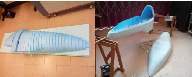
The prototype’s configuration consists in a tricycle with a front caster wheel in which the motor is built-in and two rear wheels positioned each at the tip of a tilting arm. The tilting system of the vehicle, allows it to resemble the rolling maneuver of an aircraft while turning. It presents a very distinct body’s profile with an innovative theoretical application behind its conception. The prototype’s body, shown in Figure 3.1, was first molded using Dow® Wallmate sections, then the surface was smoothen and finally covered with a glass fiber reinforced epoxy skin, in compliance with the ideals of the event which is to reduce the use of materials that depend energy intensive to produce like carbon fiber fabrics.

3.1.1

Car Specifications

In Table 3.1 the main vehicle specifications are given.

Table 3.1 - Prototype specifications – dimensions and weights.

Specifications

Dimensions [mm] Wheelbase 1027 Track/Tread (Rear) 617 Length 2461 Width 638 Ground Clearance 198 Total Height 746 Total Weight Tare Weight Prototype + 1st pilot Prototype + reserve pilot

[gf] 42983.32 96552.62 106007.4

In Table 3.2 the vehicle components weights are given.

Table 3.2 – Prototype component's weights.

Weight [gf]

Part Quantity Individual Total

Pilots 1st pilot 1 51400 51400 reserve pilot 1 60800 60800 Helmet XXS 1 1169.3 1169.3 Helmet XS 1 1224.1 1224.1 Pilot's Suit 1 1000 1000 Seat Structure 1 2900 2900 Belt 1 1389.2 1389.2

Joints and Screws 2 65.64 131.28

Chassis Structure 1 13920 13920

Front Wheel Chamber 1 83.8 83.8 Screws (Chassis-Seat) 4 14.4 57.6 Front Wheel Fork 1 1207.4 1207.4

Wheels External Cover 2 32.6 65.2 Internal Cover 2 32.4 64.8 Michellin Radial Tire 45-75R16 3 561.6 1684.8 Michelin Tire 44-406 3 225 675 Bushing and Bearings 2 916.9 1833.8

Sensor 1 2 2

Tube 16'' 3 102.5 307.5

Prototype's

Body

Fire Wall

1

113.9

113.9

Fire Extinguisher

1

1750

1750

Extinguisher's Holder

1

66.5

66.5

Joint Tubes

2

20

40

Screws Seat-Chassis

2

15

30

Screws Joint-Body

2

21.3

42.6

Canopy

Structure

1 1128 1128

Rearview Mirror

2

32.9

65.8

Mirror’s Support

2

31.98

63.96

Right Wheel Chamber.

1

61.5

61.5

Left Wheel Chamber

1

65.4

65.4

Displayer

1

23.98

23.98

Motor

Rim

1

507.8

507.8

Main Structure

1

9410

9410

Joint Parts

5

14.7

73.5

Braking

Systems

Rear Braking System

1

538.9

538.9

Pedal

1

361.6

361.6

Disk and Screws

3

125.8

377.4

Frontal Braking System

1

1200

1200

\Electronic

Joulmeters

2

500

1000

Controller

1

700

700

Cables

1

2000

2000

3.1.2

Wheels

3.1.2.1 Tires

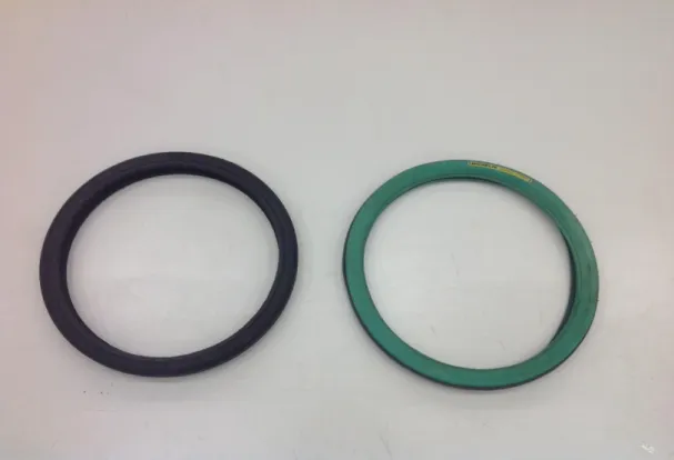
The prototype was testes with two Michelin tires that present low values for rolling friction coefficients, [4], [25], [26]: 44-406 Michelin and Michelin 45-75R16 (Figure 3.2).

Figure 3.2 – Michelin radial tires 45-75R16 (left) and Michelin tires 44-406 (right).

The 44-406 Michelin tires belong to the flexible bead area type which may, or may not, be used with a tube, inflated to a recommended maximum pressure of 5 bar (500 kPa). Radial tires Michelin 45-75R16 were specifically designed for this competition with a rigid structure without the need to use tube, inflated to a recommended maximum pressure of 7 bar (700 kPa).

In an early stage of the coasting ramp experimental tests (see Section 3.2.2) carried out to obtain values of the wheel’s bearing losses and rolling friction coefficient, the prototype was equipped first with the Michelin tires 44-406, and then with the Michelin 45-75R16 radial tires which showed, as expected, more favorable results.

3.1.2.2 Bearings

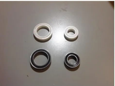
The prototype was tested with both ceramic and metallic bearings (Figure 3.3) in order to quantify the wheel’s bearing losses, as is described in section 3.2.1.

Table 3.3 - Steel and ceramic bearings' weight comparison, used by the prototype.

Ceramic Bearings Metallic Bearings

Large Small Large Small

As Table 3.3 shows, the weight’s difference between the ceramic and the metallic bearings in the present case is 21.5% for the large bearings and 22.7% for the smaller ones.

Figure 3.3 - Ceramic and metallic bearings used in the prototype.

3.1.3 Steering Gear

This prototype presents a caster wheel at the front and 2 rear wheels. The cornering system of this vehicle consists on tilting, in which the front wheel adapts to the curve trajectory, while the two wheels in the back tilt in respect to the road plane, creating the centripetal force, 𝐹𝑐, on the prototype as seen in Figure

2.9.

This system of tilting turning prevents the sideslip angle of both rear wheels and consequently no cornering drag.

The prototype was not designed for quick accelerations but rather to achieve minimum losses while turning. The prototype was designed with a negative camber angle of 6.5º. Although no experimental tests were made, this seemed an appropriate limit for low rolling friction losses, as seen in Figure 2.8 of section 2.2.5. The negative camber was implemented in the prototype to reach the ratio of vehicle high to wheel track.

The best toe angle of the prototype was also tested. The methodology will be further explained in the Ramp and Horizontal Coasting Test (See section 3.2.2). The wheels’ toe angle can be adjusted

with the aid of a screw that causes wheels arms support to change its plane and so changing the toe angle (see Figures 3.4 and 3.5).

3.1.4 Body Shape

The design of the vehicle’s body aerodynamics was the subject of a study by Fonte [24].

According to Galvão [27] it is possible to replicate in a 3D body of revolution the pressure distribution of a symmetrical airfoil along the x coordinate if a transformation of the airfoil’s Y coordinate is made for the 3D body radius, such that r=y1.5_{. This was used to depart from a purpose designed laminar flow airfoil for}

the vehicle’s Reynolds number of 1.5x106 _{in the 25 km/h design point of the car, to a 3D body of revolution.}

Then, it was assumed that the body of revolution could be altered to the prototype’s body shape as long as each cross section area was kept the same along the x coordinate (Figure 3.6).

Figure 3.6 - 3 D Cartesian coordinate system applied to the prototype.

With the aid of Software CATIA V5 and ANSYS FLUENT it was possible to obtain predictions of the drag coefficient the car prototype. These values are presented in Table 3.4 along with the specifications of the PAC-Car II that was used as a reference of performance.

Table 3.4 - Aerodynamic specs comparison, [21].

AERO@Ubi*

PAC-Car II

% (difference)

Frontal Area [m

2

_]

_0.3475

_0.254

_36.81102

Wet Area [m

2

_]

_3.586

_3.9

_-8.05128

Cd

0.085

0.075

9.893067

Drag Area [m

2

_]

_{0.028640881 0.01905}

_50.34583

F

D

[N]

0.845994372 0.810286458

4.406826

md [g]

86.32595637 82.68229167

4.406826

3.1.5

Propulsion System

The motor, controller and the vehicle’s electrical system are the work of the team member Jorge Rebelo. This is studied as his MSc theme of study, however a brief introduction is made here. The motor is an in-wheel, AC synchronous, in-wheel direct drive, with 40 pole and N52 NeFeB permanent magnets. It has an axial flux configuration with two rotors and a coreless wave winding stator made of Litz wire, as shown in Figure 3.7. The motor was designed for a cruise condition with a 96% efficient at 15W and 278 rpm. The propulsion system nominal voltage is 25.2 V provided by a 6S LiPo battery. The system has a photovoltaic cells array of 36 in series, resulting in a 18V nominal voltage that charges the battery through a DC/DC booster module.

Figure 3.7 – Propulsion system, controller and motor.

3.2 Experiments Performed

With the objective of characterizing the prototype’s performance, through the determination of the dissipative forces, several tests were performed. Hence, tests were carried out both indoors and in open environment. The indoor tests aimed to characterize the different components of the prototype alone, with no influence of other factors. These tests were conducted at the Faculty of Engineering at UBI. These included: wheel’s bearing losses tests, ramp launches and coasting tests and towing of the prototype at low speeds for direct measurement of the total dissipative force. Outdoors tests consisted of downhill coasting in roads with different slopes at Tortosendo’s Industrial Park. These tests correspond to a more advanced phase of the study, for which the prototype was tested as a whole. So, for a possible analysis of the results in different situations, it was necessary to do previous topographic measurements of the streets and launch ramp where the tests were going to be performed.

Below follows the presentation and description of the performed tests methodology as well as the theoretical background of each test.

3.2.1 Wheel’s Bearing Losses Measurement

This was the first test performed with the purpose of obtaining the wheel’s moment of inertia and bearing losses torque.

The setup consisted in a known weights held to the rim by a hook and a string. The weight was dropped from a known height as shown in Figure 3.8. The weight drop generates a final angular velocity, 𝜔, of the rim when it leaves the wheel rim. This known weight drop gives us the kinetic energy of the wheel. The time it takes to stop the wheel and the angle corresponding to the number of laps completed by the wheel allows to determine the bearing loss and moment of inertia.

Figure 3.8 – Wheel’s bearing losses measurement scheme.

Starting with the potential energy, 𝐸𝑝, of the initial position of the weight as a known energy

𝐸𝑝= 𝑚𝑤 𝑔 ℎ𝑤 (3.1)

Where 𝑚𝑤 is the weight’s mass, 𝑔 the gravitational acceleration and ℎ𝑤 the corresponding

weight’s drop. The final kinetic energy equals the initial potential energy, which means that it is equal to the potential energy of the system minus the energy losses, 𝐸𝑙𝑜𝑠𝑠𝑒𝑠:

𝐸𝑘𝑓 = 𝐸𝑝𝑖 = 𝐸𝑝– 𝐸𝑙𝑜𝑠𝑠𝑒𝑠 (3.2)

As 𝐸𝑘𝑓 is the final kinetic energy and 𝐸𝑝𝑖 the initial potential energy. Hence, we obtain the

kinetic energy this way,

𝐸𝑘𝑓=

1

2𝐼𝑤ℎ𝑒𝑒𝑙𝜔2+ 1

2𝑚𝑤𝑣𝑓2− 𝑄𝑏Ѳ𝑎 (3.3)

Where 𝑄𝑏 refers to the wheel’s bearing breaking losses torque and, Ѳ𝑎, is the angle traveled

by the weight until it separates from the accelerated wheel rim, 𝐼𝑤ℎ𝑒𝑒𝑙 the final kinetic energy,

𝜔 the angular velocity and 𝑣𝑓 the final velocity. Assuming that the acceleration of the wheel

given by the weight drop is constant, we get,

𝜔𝑖= 𝜔𝑓+ 𝛼𝑤𝑏 𝑡𝑎 (3.4)

Being 𝜔𝑖 the initial angular velocity, 𝜔𝑓 the final velocity and 𝛼𝑤𝑏 wheel’s angular deceleration

(negative value). Measuring the weight’s fall time 𝑡𝑎,

𝑡𝑎=

𝜔

𝛼𝑤𝑏 (3.5)

Knowing the division of the bearing’s torque, 𝑄𝑏, by the wheel’s inertia, 𝐼𝑤ℎ𝑒𝑒𝑙, gives the

wheel’s deceleration after the weight release, 𝛼𝑤𝑏=

𝑄𝑏

𝐼𝑤ℎ𝑒𝑒𝑙 (3.6)

Combining equations 3.5 and 3.6,

(16), (17) => 𝜔 = 𝑡𝑎

𝑄𝑏

𝐼𝑤ℎ𝑒𝑒𝑙

(3.7)

Thus we are able to write these two equations with two unknowns to determinate the wheel’s inertia and its braking torque:

1 2 𝐼𝑤ℎ𝑒𝑒𝑙 ( 𝑡𝑏 𝑄𝑏 𝐼𝑤ℎ𝑒𝑒𝑙 ) 2₊ 1 2 𝑚𝑤 𝑅2 ( 𝑡𝑏 𝑄𝑏 𝐼𝑤ℎ𝑒𝑒𝑙) 2_{− 𝑄} 𝑏 Ѳ𝑎 = 𝑚 𝑔 ℎ𝑤 (3.8) 𝑄𝑑 Ѳ𝑏= 1 2 𝐼𝑤ℎ𝑒𝑒𝑙 ( 𝑡𝑏 𝑄𝑏 𝐼𝑤ℎ𝑒𝑒𝑙 ) 2 _(3.9) As noted earlier, 𝑅2 _{( 𝑡} 𝑏 _𝐼𝑄𝑏 𝑤ℎ𝑒𝑒𝑙 ) 2_{= 𝑅}2 _𝜔2 _(3.10)

Solving in order to 𝑄𝑏 and 𝐼𝑤ℎ𝑒𝑒𝑙 we get:

{ 𝑄𝑏 = 2 Ѳ𝑏 𝐼𝑤ℎ𝑒𝑒𝑙 𝑡𝑏2 𝐼𝑤ℎ𝑒𝑒𝑙= 𝑚𝑤 𝑔 ℎ𝑤 𝑡𝑏2− 𝑚𝑤 𝑅2 Ѳ𝑏 𝑡𝑏 2 Ѳ𝑏 2− 2 Ѳ𝑎 Ѳ𝑏 (3.11) (3.12)

3.2.2 Ramp and Horizontal Coasting Test

After measuring the values for inertia and bearing losses braking torque of each wheel, two tests were made to the prototype. The first consisted in the descent of a ramp to accelerate the vehicle and coast in the horizontal straight corridor of rooms 9 at UBI.

Due to the conception of the steering system and the camber of the rear wheels, it was first intended to find the optimal tuning and best toe angle for maximal horizontal coating range and hence less rolling friction coefficient. Hence, it was measured the slope of the ramp and the length travelled by the vehicle throughout the corridor to record the distance achieved for different tuning and ramp launch positions. Notice that the beginning of the corridor corresponds to the reference point 0 of the image in Figure 3.9, where the bottom of the ramp is located. Note that the measurements were all made with reference to the travel of the prototype’s CM.

Figure 3.9 - Car coasting rolling friction test scheme.

With the aid of the Figure 3.14, we can describe the calculus process. From the vehicle’s total weight, 𝑊𝑡𝑜𝑡𝑎𝑙, and measured distances, we get the total dissipative force:

𝑊𝑡𝑜𝑡𝑎𝑙= 𝑚𝑐𝑎𝑟+𝑝𝑖𝑙𝑜𝑡∗ 𝑔

(3.13)

𝐹𝑡𝑜𝑡𝑎𝑙= 𝑊𝑡𝑜𝑡𝑎𝑙∗

𝛥ℎ𝐶𝑀

𝑙𝐶𝑀 𝑟𝑎𝑚𝑝+ 𝑙𝑠𝑙𝑖𝑑𝑒 (3.14)

Where 𝛥ℎ𝑐𝑔 is the height variation of the prototype’s CM, 𝑙𝑠𝑙𝑖𝑑𝑒 is the length slide by the

prototype and 𝑙𝐶𝑀 𝑟𝑎𝑚𝑝 is the length travelled by the prototype’s CM along the ramp. It is

possible to calculate a total dissipative force rolling friction equivalent, from (Equations 3.13 and 3.14), considering the rolling friction coefficient (Equation 3.16):

(3.13) and (3.14) => 𝑐′𝑟= 𝐹𝑡𝑜𝑡𝑎𝑙 (3.15)

𝐶𝑟=

𝛥ℎ𝐶𝑀

𝑙𝑠𝑙𝑖𝑑𝑒 (3.16)

Where the 𝛥ℎ𝐶𝑀 refers to the variation of the CM’s height due to the descent of the launching

ramp. Note that the bearing losses torque was to be negligible comparing to the wheel rolling friction torque. Therefore is was not considered in this ramp and horizontal coasting rolling friction test methodology.

The bearing losses torque, 𝐹𝑄_𝑏, generated forces of the wheels are:

𝐹𝑄_𝑏=𝑄_𝑅𝑏 (3.17)

Where 𝑅 is the rim’s radius and 𝑄𝑏 the bearing torque. To consider the influence of drag in the

test, by the conservation of energy, the speed by the end of the ramp can be found, considering, additionally the Inertia of the structure, we have

1 2 𝑚𝑐𝑎𝑟+𝑝𝑖𝑙𝑜𝑡 𝑣𝑖2+ 3 2𝐼𝑤ℎ𝑒𝑒𝑙𝜔2= 𝑊𝑡𝑜𝑡𝑎𝑙 𝛥ℎ𝑐𝑔 (3.18) Knowing that 𝜔2₌𝑣𝑖2 𝑅2 (3.19) We obtain 1 2 𝑚𝑐𝑎𝑟+𝑝𝑖𝑙𝑜𝑡 𝑣𝑖2+ 3 2𝐼𝑤ℎ𝑒𝑒𝑙 𝑣𝑖2 𝑅2= 𝑊𝑡𝑜𝑡𝑎𝑙 𝛥ℎ𝐶𝑀 (3.20)

Getting the term of velocity in evidence

𝑣 = √₁ 𝑔 𝛥ℎ𝐶𝑀 2 +32 𝐼𝑚 𝑅𝑤ℎ𝑒𝑒𝑙2

(3.21)

Assuming that the velocity drops in the horizontal corridor with a linear behavior, the mean velocity 𝑣 can be considered as 0.707 𝑣𝑖 at the exit of the launching ramp.

This leads to the conclusion that we can obtain the force of wheel rolling friction alone and the actual rolling friction coefficient,

𝐹𝑟= 𝐹𝑡𝑜𝑡𝑎𝑙− 𝐹𝐷 4 − ∑ 𝐹𝑄𝑤 (3.22) 𝐶𝑟= 𝐹𝑟 𝑊𝑡𝑜𝑡𝑎𝑙 (3.23)

Where the drag force is given by,

𝐹𝐷 = 0.5 𝜌 𝑣𝑖2 𝑆𝑥 𝐶𝐷 (3.24)

3.2.3 Horizontal Road Dissipative Force Measurements

This test consists in towing the vehicle, using a 9 meter long elastic rubber band that had a dynamometer at the end, the prototype with the pilot and the vehicle chassis without its body