An assessment of exchange rate impact over Taylor rule determination in Brazil

(1)

ALEXIS PETRI MAGALHÃES COSTA

AN ASSESSMENT OF EXCHANGE RATE IMPACT OVER TAYLOR RULE DETERMINATION IN BRAZIL

SÃO PAULO 2016

(2)

Dissertação apresentada à Escola de Economia de São Paulo da Fundação Getúlio Vargas como requisito para a obtenção do grau de Mestre em Economia

Campo de Conhecimento: Macroeconometria

Orientador: Prof. Dr. Clemens Vinicius de Azevedo Nunes

Coordenador: Prof. Dr. Ricardo Ratner Rochman

SÃO PAULO 2016

(3)

Orientador: Clemens Vinicius de Azevedo Nunes

Dissertação (MPFE) - Escola de Economia de São Paulo.

1. Política monetária . 2. Mercado financeiro - Brasil. 3. Câmbio. 4. Regra de Taylor. I. Nunes, Clemens V. de Azevedo. II. Dissertação (MPFE) - Escola de Economia de São Paulo. III. Título.

(4)

Dissertação apresentada à Escola de Economia de São Paulo da Fundação Getúlio Vargas como requisito para a obtenção do grau de Mestre em Economia

Campo de Conhecimento: Macroeconometria Data da Aprovação: __/__/____ Banca Examinadora: _________________________________ Prof. Dr. Clemens Vinicius de Azevedo Nunes (Orientador)

FGV- EESP

_________________________________ Prof. Dr. Paulo Sérgio Tenani

FGV- EESP

_________________________________ Prof. Dr. Marco Lyrio

(5)

otherwise be too burdensome to gather with consistency, and I enthusiastically acknowledge Banco Itau for supporting academic endeavors such as this one. I thank Alfredo Barbutti and Antonio Agiz and for sharing with me their lifelong experiences with the Brazilian FX markets, and BGC Liquidez for lending me their time. I also appreciate the sincere support given by professor Paulo Sérgio Tenani, from the start and throughout the year, but especially for setting up a productive session with João Lídio Bezerra Bisneto and Martin Klos-Rahal. Finally, I express my sincere gratitude to my dear friends Maurício Mirara Piesco, Cintia Maria Rocha de Oliveira and Vinicius Cropanizzo Rossi, whose patience I constantly tested on endless discussions.

I thank my advisor Clemens Nunes, for the guidance and dedication, the examining committee Marco Lyrio and Paulo Sérgio Tenani, and all the faculty of the São Paulo School of Economics of FGV.

(6)

avaliou inflação, gap de inflação, e hiato do produto, para determinar um cenario base. Sobre este, informações referentes a câmbio foram testadas. Fez-se regressões incluindo o spot de mercado e o câmbio ponderado pela balança comercial. Testou-se também o prêmio implícito em um carry-trade hipotético utilizando o primeiro futuro de dolar da BM&F. Entre as ferramentas estudadas, o "smoothing factor" foi analisado e não foram encontradas melhorias significativas. As séries foram testadas para quebras de regime, raiz unitária, cointegração, autocorrelação dos resíduos, normalidade, heteroskedasticity e linearidade de coeficientes. Entre suas características, esta dissertação leva em consideração o "timing" de cada variável. As regressões sendo "forward looking", buscou-se exatamente o valor para cada variável disponível ao Banco Central do Brasil no momento de cada decisão do COPOM. Esse mesmo cuidado foi tomado para sincronizar os dados de mercado, especialmente para construir o "payoff" do carry-trade. Esta dissertação conclui que há evidências apenas fracas de que a função resposta do Banco Central esteja em linha com a Regra de Taylor, especialmente dado o número de problemas de especificação encontrados. Os resultados também sugere que, supondo que haja a inteção de proteger a economia local de choques de fluxo de capital consequentes de mudança na taxa SELIC, o prêmio implícito no "carry-trade" não é um bom indicador desse risco.

(7)

output gap were included to determine a basis scenario. On top of that, exchange rates and exchange rate related information was tested. Both the crude market input (spot rate) and a trade-weighted currency are included in this analysis. Also extracted from the market, the carry-trade premium was calculated from future exchange rate quotes. Among its tools, the smoothing factor was evaluated. The series were tested for regime breaks, unit root and cointegration, residual autocorrelation, normality, heteroskedasticity and coefficient linearity. Among its features, special attention was paid to the proper timing of each variable. The regressions being forward looking, it was important to line up the actual information available for the Brazilian Central Bank at the time of each decision. Timing was again a factor when considering different cutoff periods, and for synchronizing market data, especially for constructing the carry-trade payoff. This work concludes that evidence of a Taylor Rule being a response function for the Brazilian Central Bank is shaky, especially given the number of misspecification indicators found. Results also suggest that, assuming there is a need to protect the local economy from sharp capital flows consequent of interest rate changes, the implicit future exchange rate premia is not a good indicator of such risk.

(8)

Graph 3 Actual SELIC target versus R#03 regression results ...43

Graph 6 Actual SELIC target versus R#05 regression results, (repeated). ...50

Graph 7 Actual SELIC target versus R#05 regression results with smoothing ...50

Graph 8 Actual SELIC targetversus the results of the R#04 regression with best performing premium series ...51

Graph 9 Actual SELIC target versus the results of the R#04 regression with worst performing premium series. ...52

Graph 10 Actual SELIC target versus the results of the R#04 regression with best performing exchange rate series ...52

Graph 12 Interest rate (actual SELIC target) series...69

Graph 13 Exchange rate series. ...70

Graph 14 Trade-weighted exchange rate series. ...70

Graph 15 Output gap series. ...71

Graph 16 Expected inflation series. ...71

Graph 17 Inflation gap series (expected inflation minus inflation target). ...72

Graph 18 IBC gap series. ...72

Graph 19 Exchange rates (blue) and all-tenor premia series (black)...73

Graph 20 Visual representation of p-values and goodness of fit measures. ...77

(9)

Table 3 Test for equality of averages between first and second periods of sample. ...30

Table 4 Interest rate series unit root tests. ...31

Table 5 Interest rate series unit root tests ...32

Table 6 Summary of unit root tests. ...32

Table 7 Summary of unit root tests for exchange-rate-related series. ...33

Table 8 Clean inflation series unit root tests. ...34

Table 9 Clean inflation gap series unit root tests. ...34

Table 10 Inflation gap series unit root tests. ...35

Table 11 Summary of unit root tests. ...36

Table 12 Cointegration tests (trace test) for the below pairs. ...36

Table 13 Cointegration tests (maximum eigenvalue test) for the below pairs. ...37

Table 14 Cointegration tests (trace test) of the 69-observations series. ...37

Table 15 Cointegration tests (maximum eigenvalue test) of the 69-observations series. ...37

Table 16 Cointegration tests (trace test) for the base regression settings. ...38

Table 17 Cointegration tests (maximum eigenvalue test) for the base regression settings. ...38

Table 18 Summary of cointegration analysis. ...39

Table 19 Regression results for R#01. ...40

Table 20 Misspecification tests for R#01. ...41

Table 29 Goodness of fit comparison between regressions. ...46

Table 30 Coefficients and significance of R#04 and R#05 with exchange rate information. ...47

Table 31 Comparison between regression with and without smoothing factor. ...50

Table 32 Misspecification results for smoothed regression. ...51

Table 36 IBC-Br generated output gap series unit root tests ...54

Table 37 Cointegration tests (trace test) for the base regression settings. ...55

Table 38 Cointegration tests (maximum eigenvalue test) for the base regression settings. ...55

Table 39 Goodness of fit comparison between regressions. ...55

Table 40 Misspecification results for smoothed regression. ...64

Table 41 Descriptive statistics of series ...68

Table 42 Coefficient values for regressions R#05 and R#04 with and without exchange rate related variables (70 OLS regressions in total) ...75

Table 43 P-values and goodness of fit for regression R#04 with and without exchange rate related variables (35 OLS regressions in total) ...76

Table 44 P-values and goodness of fit for regression R#05 with and without exchange rate related variables (35 OLS regressions in total) ...78

(10)

BM&F Brazilian exchange for futures and commodities (Bolsa de Mercadorias e Futuros)

COPOM Comitê de Política Monetária (Monetary Policy Committee, freely translating) Dilma Dilma Vana Rousseff, president of Brazil from 2011 to 2016

FHC Fernando Henrique Cardoso, president of Brazil from 1995 to 2002 IPCA Índice Nacional de Preços ao Consumidor Amplo

Lula Luiz Inácio Lula da Silva, presidente of Brazil from 2003 to 2010 TWC; TWI Trade weighted currency rate; Trade Weighted Index

(11)

1.1 OVERVIEW ...12

2. RELATED LITERATURE AND BACKGROUND INFORMATION ...15

2.1 LITERATUREREVIEW ...15

2.2 THEBRAZILIANFX MARKET ...19

2.3 THE IMPACT OF TAXES ...21

3. DATA AND METHODOLOGY ...22

3.1 SERIES ...22 3.2 STRUCTURALBREAKS ...29 3.3 UNITROOT...30 3.4 COINTEGRATION ...36 4. RESULTS ...40 4.1 REGRESSIONANALYSIS ...40 4.2 OTHERCONSIDERATIONS ...49 5. CONCLUSION ...57

5.1 POSSIBLELIMITATIONS ANDEXTENSIONS ...57

5.2 FINALREMARKS ...58

6. REFERENCE ...60

7. APPENDIX ...64

7.1 IOF CHANGES ...64

7.2 EXCHANGE RATE PREMIA- SERIES DIFFERENTIATION ...66

7.3 TIMESERIES CHARACTERISTICS ...68

(12)

1. INTRODUCTION

1.1 Overview

The financial markets offer important cues for monetary policymakers. This statement hanging by itself can be generally accepted all throughout the academia. Convergences go only this further. Since its proposal in 1993, the Taylor Rule (Taylor 1993) spawned countless works, which intended to prove it or disprove it, empirically through econometric regressions, or theoretically through working with macroeconomic equations. Regardless of controversies, it shaped the dynamics seen today: conveying clear messages of interest rate (usually through inflation targeting) in a relevant time horizon.

This work aims to build on top of that vast literature, with a focus on the Brazilian market, but the findings in this work can be extended to other emerging markets. Additionally, estimated Central Bank response function can serve as benchmark to any other response function study. This work evaluates if the additional information provided by the exchange rate derivatives market brings relevant changes to the monetary response function that took place during the Brazilian floating rate regime. In the process, it will tackle the proper timing of the data, by carefully verifying the information the BCB (Brazilian Central Bank) had at hand at the moment of the decision making. It will also assess regime breaks, and perform a thorough robustness test, something that is often overlooked when Taylor Rules are used to study monetary policy.

In the seminal article where John B. Taylor proposes the Taylor Rule, the author suggests that central banks should decide interest rates solely by looking at domestic economic conditions (disregarding exchange rates). However, one must take into account that the object of his studies was the United States, a large and developed country, and arguably the least prone to be impacted by foreign shocks. A country like Brazil, on the other hand, with a solid financial market and high interest rates, is potentially grounds to carry trade, and overall wild flows of foreign currency. In that context, monetary policy can induce large swings in the exchange rate, which in turn come back to shift the economics to a possibly unexpected outcome. This effect is studied by completely different standpoints by Molodtsova and Papell (2008), Clarida and Waldman (2008), and Engel (2016), for instance.

(13)

Aiming to anticipate the capital flows subsequent to monetary shocks, this work tests more than one FX-related information. Namely, market available spot exchange rate series, trade weighted exchange rates, and the implicit premia within the futures market. By building the last group of series mentioned, another area is touched, of equally controversial debates. This work then dives into the uncovered interest parity, the work of Fama (1984) and the several contributors that followed. The comparison of different exchange rate series, and specially the inclusion of exchange rate premia, detaches this work from past references.

Choices of variables will be detailed rigorously to avoid ambiguity, as even a slight modification in definition may lead to a completely different conclusion, as observed in the exchange between John B. Taylor and Ben Bernanke 1.

Firstly, each time series is carefully constructed (solely) with the information the BCB had at hand at the time of each decision. This approach takes to another level the view offered by Minella et al. (2002), and opposes works in which information is collected at every month-end. When a time series is composed of more than one market information, specifically the forward exchange rate premia, these market inputs are synchronized to the minute.

Finally, the robustness of each variable is tested, referring to Österholm (2003), who identified evidence of spurious regressions in his analysis. Important works, like Clarida, Galí and Gertler (2000), choose to explain why negative robustness tests were being disregarded or specific tests not taken.

Mostly, this work finds overwhelming evidence of misspecification in Taylor Rules for Brazil, including the rebuttal of the smoothing parameter (Orphanides, 1997). On foreign exchange markets, this work points out that some rates do improve results for some vertices, but don’t change significantly the misspecification findings. The exchange rate premium seems to be unrelated to monetary policy, and the analysis of the different premia series points to an absence of risk-related factor. As a byproduct, the regime break tests find sensitive evidence 1

In a public exchange of witticism – more specifically, Bernanke (2010), Taylor (2010), Bernanke (2015), Taylor (2015) – Ben Bernanke and John Taylor start debating on whether the Fed Funds rate level, in the period prior to the housing market crisis, could have led to the subsequent banking crisis. The debate then develops into which are the proper variables to be inputted into the Taylor Rule. Bernanke posts the impact of choosing between two measures of inflation, personal consumption expenditures or the GDP deflator, as they may point to two different, opposite, points. The theoretical reasoning behind either index is still up for grabs.

(14)

that monetary policy changed at some point between the first and second terms of president Luis Inácio Lula da Silva (president of Brazil between 2003 and 2010, herein Lula). By Dilma Vana Roussef’s term (president of Brazil between 2011 and 2016, herein Dilma), the link between inflation target and interest rate target are unclear, meaning the BCB and the Brazilian government secured other instruments different than short-term interest rate target as monetary and fiscal policy, and domestic currency protection.

The upcoming sections of this work are divided into the following order: section 2 reviews the related literature and clarifies the models implicit in the Brazilian financial markets; section 3 develops the structuring of the data and tests them for robustness; section 4 analyses the results; and section 5 concludes.

(15)

2. RELATED LITERATURE AND BACKGROUND INFORMATION

2.1 Literature Review

As mentioned in the introduction, this work borrows from several fields, and thus the supporting literature is quite extensive. Recall that this work aims to reproduce the (assumed Taylor-like) reaction function of the Brazilian Central Bank, using tools available in the current literature, with and without information from the exchange rate markets, and finally places the results under severe scrutiny. Section 2 is broken down into (i) studies and tools of the Taylor Rule, (ii) studies that analyze the relationship between the exchange rate and the interest rate, and (iii) foreign exchange premia.

The cornerstone of this work is set by John B. Taylor (1993), who originally proposed the Federal Reserve were, intentionally or not, following a simple rule-of-thumb for setting short-term interest rates. Taylor points to only three variables: inflation, inflation target and output gap. Orphanides (1997) then poses the question of what the Fed has to work with, breaking away with the habit of looking at past variables, choosing forecasted variables instead. Minella et al. (2002) poses that same concern, using as the inflation variable from the official forecast disclosed by the BCB (the quarterly Inflation Report). They apply special effort to inflation, opening the paper with its drivers, including year targets for their regressions. The two-year target may seem a stretch from the – understandably – “ad hoc” mindset of Brazilian policymakers. Notwithstanding, the overall handling of inflation was mostly kept herein. The same logic – of reproducing the BCB’s “by then” standpoint – is applied here, not only for inflation, but for all other variables, especially market related, where information may change from day to day.

Still on the basic Taylor Rule, two tools are borrowed from previous researchers. One of those improvements was brought by Orphanides (1997), as well as Clarida, Galí and Gertler (1997), and Rudebusch (2002), the smoothing factor. In these works, the rule’s equation is rearranged to account for the tendency of the Fed (and other central banks) to smooth out sharp interest rate changes, often leaving a portion of the past decision (hike or reduction) to the upcoming meeting. This inclination brings efficiency to the financial markets, for it reduces the need of interest rate risk hedging. Differently from the aforementioned works, however, this work

(16)

compares regressions with and without the smoothing factor, and finds no significant change. Most importantly, it finds no improvement in the misspecification tests.

Misspecification tests are not a side track of this study. Österholm (2003) calls for rigor when analyzing the econometrics of the Taylor Rule, and his work provides a framework for the tests with Brazilian data. He gathers data from the United States, Sweden and Australia, and finds persistent indicators that the relationship mapped as a central bank behavior may be spurious. Some of these indicators are also found for the Brazilian data, such as serially correlated residuals and mixed results on cointegration. However, tests on Brazilian data find even more concerning problems. It finds heteroskedasticity as a misspecification, for instance. It will be shows that these findings are persistent, and including exchange rate variables in a Brazilian estimated response function does not improve these issues.

Another borrowed tool is the breakpoint test. Judd and Rudebusch (1998) apply it to compare inflation aversion and output gap aversion of the Fed chairmen Arthur Burns, Paul Volcker and Alan Greenspan, and find different coefficients. They set precedent for others, including some in the Brazilian academia. This section recalls two of those works: Salgado, Garcia and Medeiros (2005) and Barcellos and Portugal (2007).

Salgado, Garcia and Medeiros (2005) applied a Taylor-like rule to the 1990’s period. They modeled the interest rate series into a regime switching time series, where it goes from “tranquil periods” (to use their terms) to more volatile periods during the crises of Mexico (1994-95), Asian markets (1997) and Russia (1998). The threshold variable chosen was international reserves. It triggers a crisis start when the accumulated three-month change drops below the threshold. Minding that their analysis horizon encompasses one year of floating-rate policy, including the turbulent switch and subsequent adaptation, they point out that the change in international reserves is a good indicator of a crisis only under the fixed-rates regime. Their model seems to correct some misspecification errors. This work does not use exchange rate information as a threshold variable, but it will be seen in the results section that, with the correct filter, future research might find a threshold-type of variable within the exchange markets instruments.

Barcellos and Portugal (2007) use the Taylor Rule approach to determine if there is a regime break between the BCB chairmen Fraga’s and Meirelles’ periods, or between former presidents

(17)

Fernando Henrique Cardoso (president of Brazil between 1995 and 2002, herein “FHC”) and Lula. Since his election, FHC had a turbulent second mandate, including the unwindings of the Asian Crisis (1997), Russian Crisis (1998), US’s dot-com bubble burst (2000), Nine-eleven (2001), the Argentinian Crisis (2002) and the Brazilian Energy Crisis (2002). When former president Lula takes office, he promises to break away with FHC’s economic policy. Barcellos and Portugal use a dummy variable to conclude that such break did not occur in the examined period. Interestingly enough, the authors stumble upon mixed signals over the impact of exchange rate. Looking solely at the BRL to USD exchange rate, they conclude that “this effect […], when analyzed separately, turned out to be moderate, which must be related to the indirect influence of this variable on other pieces of information used in the models.” As a first takeaway, a regime break is found both through dummy variable and coefficient comparison. The second takeaway is the hinted influence of exchange rates in the Taylor Rule. On evidence of such influence, Barcellos and Portugal do not stand alone.

The concept of using exchange rates combined with Taylor Rules is not in all new. Minella et al (2002) point to inflationary pressures of the exchange rate. Clarida and Waldman (2008) studied the impact of inflation-related news to the exchange rate, and find such impact to be relevant for inflation-targeting countries. On this work, however, only ten developed countries were studied (no emerging markets). Other studies with exchange rates on Taylor Rules include Devereux and Engel (2007) and Huang, Margaritis and Mayes (2001). The first attempts to model how news on terms of trade anticipate exchange rates movements, and may be targeted by inflation-setting countries. The latter include a trade-weighted index as proxy of an exchange rate on the policy rule of New Zealand, supported not only by the inflationary pressures of the exchange rate in a country with capital mobility, but also by the explicit defense of a stable currency from the Reserve Bank of New Zealand.

Hand-in-hand with this approach, but from a different perspective, Engel, Mark and West (2008) have achieved some predictability on real exchange rates by assuming a system of equations in which two countries work with the Taylor Rule, and where the purchasing power parity (PPP) holds. Similarly, Molodtsova and Papell (2008) find promising results for exchange rate predictability, by building a binary system in which two countries simultaneously set interest rates by targeting inflation, and where uncovered interest parity holds. Moreover, it’s been mapped by Eichenbaum and Evans (1995), Engel (1996, 2016), and Barroso, Silva and Sales (2013), that domestic decisions on interest rates, and foreign decisions

(18)

as well, impact the exchange rate as increasing (or decreasing) onshore rates produce a significant and persistent appreciation (depreciation) on the local currency. The hike, for instance, magnifies instead of dampens the gains foreign capital has on interest rates.

All the above works show the link between exchange rate and monetary policy, and fueled the inclusion of an exchange rate related variable to the Brazilian response function in this work. To the standpoint of this author, a higher interest rate differential attracts capital in the form of carry-trade. If a hike in rates, for instance, accelerates to some extent the inflow of foreign capital, the pass-through effect to inflation may overdo the BCB’s goal. On the other hand, to defend the currency, the sterilization needed may partially undo the tightening of an interest rate hike. This work then needs an indicator of the likelihood of capital inflow (outflow) at a given interest rate increase (reduction).

In his acclaimed work, Fama (1984) points to the existence of a time-varying premium, which is the difference between the future exchange rate and the market expected value of the exchange rate in the future. In his demonstration, covered interest rate parity (which postulate that the difference between future and spot exchange rates must be linked to the interest rate differential between the two countries) holds2. Future and spot prices have to be tied in a way that there can be no arbitrage to shorting a bond in a country, buying a bond in another currency and selling its payoff-worth of future currency. However, there is profit opportunity in performing the described operation, with or without locking in the payoff with future exchange rate contracts (though the risks, and consequently the profits, vary). Without negotiating future exchange rate contracts, what surfaces is the aforementioned premium. In the 1990’s and 2000’s, the academia shifted its focus to identifying what is that premia.

Froot and Thaler (1990) characterize the premium not as a risk indicator, but as a product of “delayed overshooting”, for it is costly and time-consuming for investors to readjust their portfolios. Verschoor and Wolf (2001) use survey data to find evidence of a risk premium in the premia for Scandinavian currencies. However, Frankel and Poonawala (2010) find that the bias is lower for emerging market currencies, which are naturally more volatile. While that would point out to absence of risk premia, they admit that the existence of bias is left

2

Though Fama uses bonds in his argument, this work will apply the same rationale to short-term interest rates. It will become clear throughout this document that the Brazilian Market is predominantly a short horizon market.

(19)

unexplained, and conclude that “the source of forward discount bias does not lie entirely in the exchange risk premium.”

Sarno, Schneider and Wagner (2012) expand the concept, working with a risk-adjusted forward unbiasedness hypothesis (which, if held, would say that the forward rate is an unbiased predictor of the future spot rate) and a risk-adjusted uncovered interest parity. They create a time-varying premium series which, in combination with an interest rate differential series, seem to explain exchange rate movements. They conclude that “risk premiums can be sufficient to resolve the forward bias puzzle without additionally requiring departures from the rational expectations.”

One approach would be gathering market survey data for Brazil on expectations of future exchange rates. However, to avoid running into the issue of the low forecasting power of such surveys, this work constructs its premia series as exceeding cash in an actual carry trade. This premia would also be a product of a sovereign risk or liquidity risk and/or market imperfections (frictions or a collapse of the rational expectations hypothesis). In that sense, an original contribution of this work is the specific market approach on calculations. All comparisons and conclusions take into account the correct timing of the inputs and the exact payoffs of the financial instruments available for the market agents. Wherever cash is unencumbered to be transacted, the calculations will imply its flow. Only then one can properly evaluate if this premium reflects the eagerness of foreign investors to invest in Brazil. Section 4 finds that the connection between the premia series and the Taylor Rule is highly dependent on the timing of the measurement, which suggests no hidden component in the forward exchange rate premium.

To ensure absolute clarity of the financial instruments available, and its proper use, the Brazilian market is carefully detailed in the following subsection.

2.2 The Brazilian FX Market

During the transition from fixed to floating currency, the Brazilian spot market was flooded by all sorts of counterparties, from banks to pension funds and individuals. In a context of a market crisis – the fixed currency policy collapsed as an aftermath of the Asian and Russian crises – the excess liquidity resulted in wild volatility. To counter that, the Brazilian Central Bank (BCB) created the exchange portfolio, freely translating. Only banks would be eligible to

(20)

apply for a grant to have an exchange portfolio, and only those with accepted applications would be allowed to operate in the Real-Dollar spot market, and hold a position in offshore currency. The transactions in the spot market must be informed to the BCB by the end of the day. These banks are known – and hereafter referred to – as dealers.

The exchange portfolio still exists (during these last years, though, brokerage houses have been allowed to operate on the spot exchange up to $250 thousand). Such tight regulation has drained the spot market of its liquidity, leading brokers, banks and pension funds to migrate to the futures market, that requires only a clearinghouse account and margin deposits. Ventura and Garcia (2012) measured the Brazilian currency futures market to be five times bigger than the spot market during 2006-2007. By this time, the Bank for International Settlements (BIS) placed Brazil with the second biggest exchange-traded currency derivatives market in the world3.

With all other players dependent on dealers to operate US Dollars within Brazil, and drawn into the futures market, they are given access to the spot market through a synthetic instrument called CASADO, which is the purchase (sale) of the first future combined with the sale (purchase) of the spot. These are dealt by brokers, and must be cleared by a dealer before the end of the day. The price of the first future, for margin call, is set between 15:50 and 16:00. This dynamics points to the need of synchronizing the price setting of the spot and first future, at 16:00 Brazilian Time.

Futures contracts traded in BM&F (Bolsa de Mercadorias e Futuros, Brazilian exchange for futures and commodities) have a band within which the price is allowed to move. Circuit breakers are a common way for the stock exchanges to protect themselves against volatility shocks. The spot market, however, does not have any limitation, so wild swings break up the relationship between spot and futures prices, and distort further analysis.

Summarizing the instruments and market indexes of interest of this work:

3

The BIS Quarterly Reviews (produced by the Bank for International Settlements) consistently portraits Brazil among the top ten most active exchange-traded derivative markets, both for interest rates and exchange rates. This reinforces the relevance of studying Brazil as an active playfield of carry trade.

(21)

a) Spot market: Purchase or sale of the Dollar against Real, with usual delivery in two days. The spot market, differently from the futures market, does not have any form of circuit breaker.

b) First future: Future contract of the Dollar against Real. First future matures on the first business day of the upcoming month, at which point there is no physical delivery (it is settled in Brazilian Reais). According to Ventura and Garcia (2012), this contract accounts for 85% of FX futures market volume4.

c) CASADO: Synthetic instrument composed by the purchase (sale) of the first future combined with the sale (purchase) of the spot.

d) Libor: Interbank offer rates, surveyed by the Intercontinental Exchange (previously, by the British Bankers Association). For this work, it is assumed that this rate would fund a carry trade deal of Brazilian Reais against US dollars.

e) SELIC target: Short term interest rate target, set by the COPOM, for overnight repurchase agreements of federal bonds. Similar to the US’s Fed Funds.

2.3 The impact of taxes

Before translating the described background into the framework to build the series used for the upcoming analysis, the reader must be aware that Brazil has a long tradition of complex and ever-changing taxation regimes. Furthermore, decrees were issued between 2007 and 2013, roughly, some aimed at specifically the trade of concern for this work.

One tax in particular, the IOF, was aimed to make short-term carry-trade more expensive. The rule, however, changed several times, forcing the markets to adjust (which may have occurred during unknown timeframes). Though the payable taxes are not quantified in this work, regulatory impacts on the markets have been pinpointed and are taken into consideration when evaluating statistical conclusions. A summary of those changes may be found in Exhibit 7.1 of the appendix. The complete breakpoint analysis finds, in the future sections, that as taxation changes became more frequent, inflation targeting became less of a norm.

4

To assess premia on tenors longer than one month, BM&F’s off-the-shelf FRC contracts were considered. Through FRC contracts, participants trade interest rate differential, in US Dollars, between the first business day of every month and the first business day of the upcoming month. Stripped out of the spot and the interest rate in Brazilian Reais, this contract implies a future of the exchange rate. Unfortunately, lack of liquidity halted this approach.

(22)

3. DATA AND METHODOLOGY

3.1 Series

This section describes the construction of the series used in this work.

The fixed rate regime was withdrawn in Brazil starting on January 1999. In June, decree 3088 established inflation targeting as the new monetary regime, with specific dates for determining the next year’s target and tolerance bands, and for justifying any past non-conformities, in an open letter from the BCB to the Brazilian government. With this in mind, the data for this work spans from July 1st, 1999, to June 30th, 2016.

Conceptually, the base equation of the Taylor rule, over which this work unwinds, is represented by below equation.

(1) = + + + + ф +

Being, i: Target rate set by COPOM (Monetary Policy Committee, freely translating), known in Brazil as Meta Selic;

π: Expected year-end consumer inflation, to which the BCB target is set against (yearly percentage change of the Brazilian index IPCA – Índice Nacional de Preços ao Consumidor Amplo);

πgap_{: Deviation from inflation target (expected end-of-period consumer inflation}

π minus end-of-period BCB-set target; ygap: Output gap;

ϕ: Exchange rate scenarios (explained further); ε: Error term;

The base equation, the regular Taylor Rule, is a function of inflation, the difference between expected inflation and inflation target (that will be referred to simply as “inflation gap”) and output gap.

(23)

The output series chosen was the monthly IBGE-measured industrial production, seasonally adjusted. The output gap is the percentage difference between the aforementioned series in crude form, and that same series filtered by Hodrick-Prescott decomposition, in a way that a negative value of output gap means idle production capacity. Output gap was also evaluated from the IBC-BR released by Central Bank, as an alternative.

Inflation and Inflation targets were extracted from public information disclosed by the Brazilian Central Bank. As briefly discussed in section 2.1, inflation forecasts were collected from the quarterly Inflation Report, elected to reflect the BCB’s by-then expectations at year-ends. The concept behind forward-looking inflation is fairly simple, inflation targeting is by definition forward looking, and past inflation is not necessarily a good predictor of future inflation. With this in mind, Minella et al. (2002) gather their series from the Inflation Reports, quarterly produced by the Brazilian Central Bank (BCB). For this work, each quarterly Inflation Report was read and analyzed, and the inflation series elected reflects the BCB’s expectation at year-end. Different from Minella et al. (2002), targets other than current years are assumed to have no weight on the decision.

The exchange rate related series are described in more detail. Recalling equation 1, the five scenarios (ϕ) are elaborated as follows.

a) A null series (i.e. the standard Taylor Rule);

b) Each of the 11 FX premia series, recorded at uniform distance from the next future’s settlement date;

c) Each of the 11 exchange rate series, recorded at uniform distance from the next future’s settlement date;

d) Each of the 11 exchange rate series, recorded at uniform distance from each COPOM meeting;

e) A trade weighted exchange rate, recorded at a uniform distance from each COPOM meeting.

The second rule tested (b) includes the FX-implicit premia. It is herein called “premium” the implicit yield in the difference between the first future and the spot of the US Dollar to Brazilian Reais. The reasoning behind including the premia in the monetary policy recipe assumes there is a risk component to it. High premia allow for more elastic interest rate hikes,

(24)

as it is less likely these hikes will produce an inflow of dollars, and alter the effect of the contractionary policy.

Note that the premia series are composed of observations grouped together with respect to the distance to the next future’s settlement date (for reasons that will become clear when discussing the construction of the premia series). As a consequence, the observations within a series – say, the 20-day tenor series – will have all sorts of dates, not equidistant from the COPOM meeting dates (and most definitely not the end of month). The third scenario follows that logic, it is the value observed at a specific business-day distance from the next future’s settlement.

If in the third scenario (c) the exchange rate observation window is synchronized with the premia observation window, for the fourth scenario (d), the COPOM meeting dates are taken as reference, from 2 to 12 business days (Brazilian calendar) of the announcement of the new SELIC target. The shortest distance, 2 business days was chosen to respect the duration of the meeting, which lasts two days, taking into consideration the necessary time to measure that variable and produce reports to steer the committee.

In other words, a x-tenor exchange rate series will have grouped all exchange rates observed at 16h00 of a day that was x business days away from a first-future contract’s settlement date. Each element t refers to a COPOM decision, so the t-th element of such series is the last observation that happened before the t-th COPOM decision. In that sense, the observations in x-tenor ER are all equidistant from future’s maturities, but not from COPOM dates. The second exchange rate (T-offset ER) is the rate observed at 16h00 of the day that is T business days earlier than t. Thus, the observations in T-offset ER are equidistant from the COPOM dates, but not from the first future’s maturity. The two different exchange rate series are built to ensure surfacing of a possible accidental synchronization of exchange rates observations, which could produce an artificial relationship. This hypothesis is scratched off in the following chapter, as the two exchange rate series produce similar results.

Another exchange rate series is constructed using the Trade Weighted Index put together by Morgan Stanley Inc. The series is an index of USD per BRL with base 100, so the series is divided by 100 and inverted to BRL/USD. This information is set public through Bloomberg L.P. This information is only available from January 2000 onwards, so every regression and study with this variable was cropped short of its observations.

(25)

The construction of the premia series is conditioned to data availability. Synchronized time-series are public information, but require processing power for the non-constant data pattern from the clearinghouses, and rigorous record-keeping. The synchronized data, exchange rates at spot and future contracts, were obtained from Itau Unibanco. After producing the aforementioned synchronized time series of first future and spot prices, gaps may be filled with a CASADO price series available in Bloomberg LP. This information was not chosen to be the primary source for it is not observable in the market; rather, it arises from daily survey with Bloomberg’s feeders.

The aforementioned grouping of elements in each premia series produced 24 time-series, ranging from 3 to 26 days span between spot and future maturity. It was taken into account the specifics of the cash transactions involved in the trade, i.e. following business day (“d+1”) of the purchase, on the Brazilian calendar, and d+2 of maturity, skipping to the next business day when d+2 lands on a US holiday.

The first-future-to-spot differential is translated into a per annum rate, adapting to the Brazilian calculation method of settlement values. Covered interest parity dictates that the difference between the forward and spot exchange rates observed at t is directly related to the difference between the interest rate on nominal bonds denominated in the two currencies. However, given the short-tenor nature of the instruments used, this work resorts to the risk-free yield curves of Brazil (Pre) and USA (Libor).

(2) = ,

, / − 1 ∗ − ,

Being, ρt: Premium at day t;

Ft,T: First future price at day t, maturing in T business days; St,T: Spot price at day t, being Reais to a Dollar;

Pt,T: Quoted annual rate of the Brazilian risk-free yield curve for tenor T; Lt,T: Quoted annual rate of the US risk-free yield curve for tenor T; Tcd: Tenor T in calendar days;

(26)

The formula is justified by the calculation standards of each market, namely, linear rate on calendar days over 360 for Libor and exponential rate on business days over 252 for Pre. This approach ensures that the calculated dollar premium is as close to what is feasible, using the Fed-set ceiling rate as an anchor, or reference rate5, which almost coincides with an interpolated Libor rate.

The above formula produces 24 time-series, for tenors ranging from 3 business days to 26 business days. There was no attempt to rejoin the 24 different series back into one. This is further explored on Exhibit 7.2.

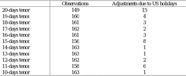
Series 26 to 21 were removed from the set due to lower-than-average number of observations, and series 9 to 3 were excluded for having higher-than-average variance. Omitted from the exhibits, an F-test for equality of variances was performed for every two pairs of series. Each of the series between 9 and 3 had the null rejected for most if not all the tests against the other 23. For further clarity, there are three reasons why one series would have less observations than others: unequal-sized months, national holidays, and lack of data. After filtering out the 13 series above, the 11 series remaining still were uneven in size. These dates, theoretical inceptions of carry-trades, landed on US holidays, thus no anchor rate and no real trade opportunity. These values were filled out with data from previous day, and the premia were calculated normally. To keep track of this approximation, the number of adjustments made to each series is recorded in Table 1.

5

Two groups of time-series were created, with and without an anchor. As expected, time-series without anchors have higher variance than those without one. Since this conclusion seems intuitive, the author refrained from including the latter in this work. All data is available upon request.

(27)

Table 1 Number of observations and adjustments for each series of implicit premia.

Observations Adjustments due to US holidays

20-days tenor 149 15 19-days tenor 160 4 18-days tenor 161 3 17-days tenor 162 2 16-days tenor 161 3 15-days tenor 156 8 14-days tenor 163 1 13-days tenor 163 1 12-days tenor 162 2 11-days tenor 158 6 10-days tenor 163 1

Worth noting, from July 1999 to June 2016 including, there are 204 months. However, not all months witnessed rate setting. There were 164 COPOM meetings during those 204 months, so each time-series had to have necessarily 164 observations at the respective specific days. The data was grouped as to reflect the information COPOM had at hand by the time of the decision. In that way, information regarding FX-implied premia available may have been of current or previous month, depending on the day of the meeting. Information on BCB-expected inflation may have been of up to three months prior to the meeting, depending on the reports’ release dates. Same goes for production gap and so on.

There are situations in which COPOM sets multiple rates for different time horizons. Between June 1999 and July 2016, there were two meetings like that, each with two different rates at once. Since the set of information available was identical at each decision, the two different rates cannot be each considered a separate observation. These meetings were not excluded altogether, but the last rates were privileged. The decision was made taking into consideration the trend: in both cases there were short-lived rates which suggested an intermediate step into achieving the desirable rate. These two intermediate rates were thus excluded from the set.

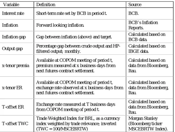
The series are graphically reproduced on Exhibit 7.3, together with its descriptive statistics. Table 2 summarizes the variables evaluated in this work.

(28)

Table 2 Definition and source of each variable.

Variable Definition Source

Interest rate Short-term rate set by BCB in period t. BCB.

Inflation Forward looking inflation. BCB’s Inflation

Reports.

Inflation gap Gap between inflation (above) and target. Calculated based on BCB data.

Output gap Percentage gap between crude output and HP-filtered output; monthly.

Calculated based on IBGE data.

x-tenor premia

Available at COPOM meeting of period t, premium measured at x business days from next futures contract settlement.

Calculated based on data from Bloomberg, Itau.

x-tenor ER

Available at COPOM meeting of period t, exchange rate observed at x business days from next futures contract settlement.

T-offset ER Exchange rate measured at T business days from COPOM meeting of period t.

T-offset TWC

Trade Weighted Index for BRL, as a currency index weighted by trade relevance; inverted (TWC = 100/MSCEBRTW)

Morgan Stanley (Bloomberg ticker MSCEBRTW Index).

As will be seen further on, varying the T-offset did little to alter the results. That said, there will be only one trade-weighted exchange rate series (5-offset), instead of 11.

Having the relevant time-series at hand, it becomes mandatory to undertake robustness tests at each empirical result. Section 4 will take the reader step by step through the analysis of the data itself, and the relationships being investigated.

Österholm (2005) raises the question of how likely it is for a Taylor Rule estimation to fall into a spurious regression. In line with his work, the steps taken here are as follows.

a) Series are analyzed for structural breaks, taking breakpoint candidates and assessment methods from works of Judd and Rudebusch (1998) and Barcellos and Portugal (2007). First the series are tested with Chow test. Then, two regressions are done separately, and their coefficients are tested for equality of means through the Welch test.

b) All series are tested for unit root through the Augmented Dickey-Fuller test, herein referred to as ADF, which has a unit root as the null hypothesis, and the

(29)

Kwiatkowski, Phillips, Schmidt and Shin test, or KPSS from now on, which has stationarity as the null hypothesis.

c) Non-stationary series are tested for cointegration with the Johansen tests. Since the Johansen tests assume normality, residuals are put under the Jarque-Bera normality test. This test, together with all other regression robustness tests, will be further clarified in the following section.

The software used in section 3 was the PCGive and GARCH (for KPSS test only) modules of OxMetrics version 5.10, except the Chow test, Quandt-Andrews test, and Johansen tests on multiple regressors, for which Eviews 7 was used.

3.2 Structural Breaks

Previous works have tested whether a change in a central bank’s chairman implies a structural break. Judd and Rudebusch (1998) compare the coefficients of the three Fed chairmen that held office from 1970 to 1997. Barcellos and Portugal (2007), as mentioned earlier, use dummy variables to conclude (by lack of significance of the coefficient) that there is no regime break when switching chairmen (and simultaneously, presidents, namely FHC and Lula).

In Brazil, several economists have pointed out a significant break from past economic policy at Lula’s second term onwards, into the government of former president Dilma, i.e. from January 2007 onwards. Setting January 2007 as a breakpoint candidate on a Chow test produced the rejection of the null of coefficient stability (for this test, the regression used was the one of Model 1, that is, with ϕ as a null vector). Around the same time, two other events occurred that may have triggered a regime break. Before 2007, former Finance Minister Guido Mantega replaced his predecessor, Antonio Palocci, in March 27th, 2006. After 2007, the US housing market collapsed and a crisis unwound. These two breakpoints were also tested, and evidence of structural breaks was found. Considering the small amount of observations in between these dates, the similar results are understandable6. The Quandt-Andrews test found a regime break in the constant, inflation gap and output gap at around July 2006, in line with expectations.

6

There are six observations between March 2006 and January 2007, and there are seven observations between January 2007 and January 2008.

(30)

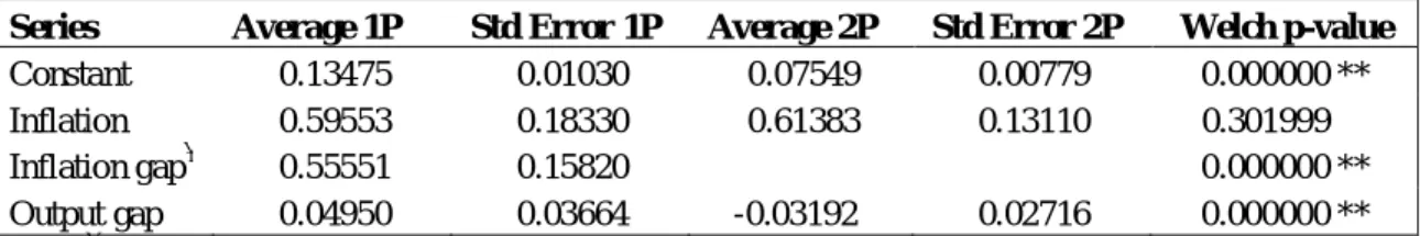
As a third test, two different regressions were run with Model 1, for two different time periods, and the statistical significance of the equality hypothesis between each of the coefficients was evaluated (Welch’s t-test). There is sufficient evidence of a structural break, the results are as follows.

Table 3 Test for equality of averages between first and second periods of sample.

Series Average 1P Std Error 1P Average 2P Std Error 2P Welch p-value

Constant 0.13475 0.01030 0.07549 0.00779 0.000000 **

Inflation 0.59553 0.18330 0.61383 0.13110 0.301999

Inflation gap҂ 0.55551 0.15820 0.000000 **

Output gap 0.04950 0.03664 -0.03192 0.02716 0.000000 **

Note:҂ Inflation gap turned out to be linearly dependent to inflation on the second period, and thus was excluded. Note: Periods 1 (1P) goes from 1999 to 2006, period 2 (2P) goes from 2007 to 2016.

Note: One and two asterisks (* and **) stand for rejections at 5% and 1% respectively.

The Welch test rejected equality of means for all coefficients other than inflation. The constant being rejected comes to prove that the real interest target shifted at some point in between Lula I and Lula II. Inflation gap during the second period is linear dependent on inflation, and thus has to be removed from the second regression. The shown equality of treatment for inflation between periods one and two reiterates the validity of the test in this context. Hypothesizing equality may be too strong of a proposal, especially given that it assumes normality, then failure to reject it for inflation offers comfort that this approach is not being excessively conservative. Interestingly, output gap shifts signs. A negative sign in the coefficient would mean the COPOM is being contractionary (or expansionary) when the economy is weakening (strengthening). Worth mentioning, in neither regressions (of periods one and two) output gap is significant.

In light of these results, the breakpoint date chosen was January 1st, 2007. From this point onwards, some series will be mentioned to be of “Period 1” or “Period 2”, meaning from July 1999 to December 2006 and from January 2007 to June 2016, respectively.

3.3 Unit Root

All series were put under unit root test to assess the likelihood of spurious regression. Akaike information criteria was chosen to determine the optimal lag length for the ADF test. The use

(31)

of ADF itself is hardly ubiquitous. For instance, Österholm (2003) gives much more credit to the power of the test than do Clarida, Galí and Gertler (2000), as will be mentioned in more detail shortly. To strengthen the analysis, KPSS test was also used as alternative to the ADF, with the remark that the ADF has the null hypothesis of a unit root, while KPSS has the null hypothesis as stationarity.

The short-term interest rate target series, the independent variable of all upcoming regressions, does not seem to be stationary. The ADF test and KPSS both place it as an I(1) process, as seen below (table 4). This result ties with past analysis. Salgado, Garcia and Medeiros (2005) have tested an uninterrupted (one regime) interest rate series, and put it against a regime-shifting interest rate (the series intercalates “tranquil” periods with four “crises” periods). They have found it not to be stationary, while evidence of unit root did disappear for the crises series. That would not necessarily be the case for the series used in this work. The path of Brazilian interest rates during the nineties – a decade in which the country stabilized its economy and finally put an end to the hyperinflation – is hardly related to the one observed in the following years. Interest rates had surpassed 80% during the Mexican crisis, and sloped down to smooth 20%’s by mid-1999. The fact that the interest rate series is I(1) from 1999 to 2016, just as it were from 1994 to 1999, is rather noteworthy.

Table 4 Interest rate series unit root tests.

Interest rate t-stat 5% 1%

ADF Level -1.101 -2.88 -3.47

ADF First diff. -5.995** -2.88 -3.47

KPSS Level 3.545** 0.463 0.739

Note: ADF has the unit root as the null hypothesis, KPSS has stationarity as the null hypothesis.

Breaking the interest rate series into two series, referring back to the regime break between Lula I and Lula II, produces similar results for the ADF. Table 5 evidences the test failing to reject the null for level. KPSS responds differently, however, also failing to reject its null of stationarity.

(32)

Table 5 Interest rate series unit root tests t-stat 10% 5% 1% P er io d 1 ADF Level -0.541 -2.9 -3.51

ADF First diff. -4.757** -2.9 -3.51

KPSS Level 0.278 0.347 0.463 P er io d 2 ADF Level -0.355 -2.9 -3.52

ADF First diff. -2.748 -2.9 -3.52

KPSS Level 0.371 0.347 0.463

Note: Period 1 stands for 1999 to 2006 (FHC II + Lula I) and Period 2 stands for 2007 to 2016 (Lula II + Dilma). Note: One and two asterisks (* and **) stand for rejections at 5% and 1% respectively.

These results shouldn’t be much of a concern. Reducing to half the quantity of observations should severely impact the power of the tests. In that context, results are mixed. Once again, a similar development was observed by Salgado, Garcia and Medeiros (2005).

Finally, as will be seen further down this chapter, inflation gap and output gap did not prove to be significant in explaining the second period of interest rate. Nonetheless, cointegration was tested for the split series.

Having tested the interest rate series, all other series are tested. The summarized results are as follows.7

Table 6 Summary of unit root tests.

Series ADF KPSS

Inflation 5% 5%

inflation gap 5% 10%

1st P inflation gap 5% 1%

2nd P inflation gap 10% 1%

output gap 1% doesn't reject

1st P output gap 1% doesn't reject

2nd P output gap 1% doesn't reject

Note: Period 1 (“1P”) stands for 1999 to 2006 (FHC II + Lula I) and Period 2 (“2P”) stands for 2007 to 2016 (Lula II + Dilma).

Table 7 summarizes the unit root tests for the series with exchange rate information.

7

The specifics of the tests are not included in this document, but are available upon request, together with the series themselves.

(33)

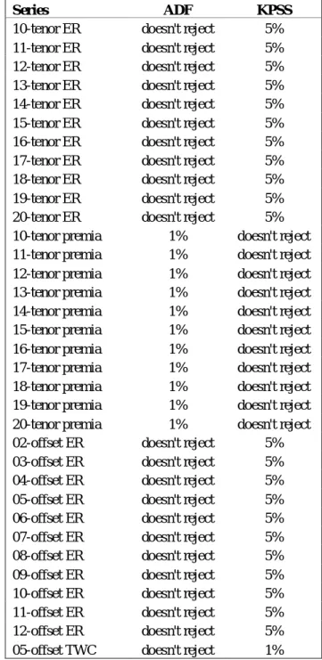
Table 7 Summary of unit root tests for exchange-rate-related series.

Series ADF KPSS

10-tenor ER doesn't reject 5%

10-tenor premia 1% doesn't reject

02-offset ER doesn't reject 5%

05-offset TWC doesn't reject 1%

Interestingly, the exchange rate and interest rate are not I(0) processes, and should be tested for cointegration. These results are hardly ground-breaking for monetary policy. Clarida, Galí and Gertler (2000) argue that, in the long run, theoretical plausibility should thrive over empirical inobservance. Nonetheless, from a statistical standpoint, such empirical constrain can very well spoil overall results.

(34)

Inflation and inflation gap were put under special scrutiny. Recalling that the Inflation Report is quarterly disclosed and the COPOM meetings are every 42 days approximately, each observation is potentially repeated. From July 1999 to June 2016 there were published 69 Inflation Reports. Hence, the original inflation series have duplicate values (or triplicate values) in its 164 observations. Alternative series of inflation and inflation gap were constructed for some tests, each with 69 observations. These series will be referred to as “clean series” as opposed to the “original series”, not to be confused with “cropped series”, referring to the inflation gap series with values for first period only (1999 to 2006), and zero otherwise.

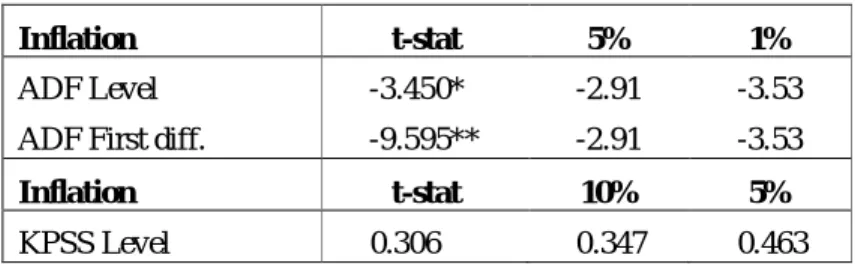
The ADF test rejects the null hypothesis of unit root at 2% of inflation in level. Worth noting, the ADF test does not reject the unit root hypothesis if a constant is not included in the AR process. However, the assumption that inflation is not a pure random walk process seems safer than assuming otherwise. Accordingly, KPSS test does not reject the null hypothesis of stationarity.

Table 8 Clean inflation series unit root tests.

Inflation t-stat 5% 1%

ADF Level -3.450* -2.91 -3.53

ADF First diff. -9.595** -2.91 -3.53

Inflation t-stat 10% 5%

KPSS Level 0.306 0.347 0.463

Regarding inflation gap, in level, the null hypothesis of unit root is rejected at 5%. Table 9 Clean inflation gap series unit root tests.

Inflation gap t-stat 5% 1%

ADF Level -2.242* -1.95 -2.60

ADF First diff. -8.381** -1.95 -2.60

Inflation gap t-stat 10% 5%

KPSS Level 0.240 0.347 0.463

(35)

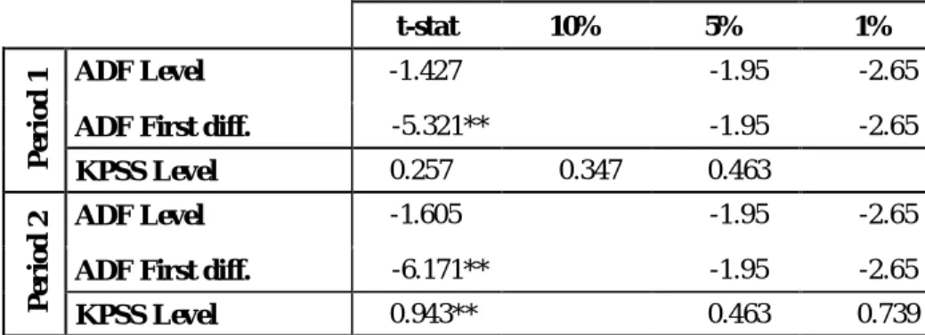
Considering this variable is apparently only relevant during the FHC-Lula I period, a cropped series was also tested (up until December 2006, 31 out of 69 observations remain). Stationarity is unequivocally rejected at 1%. This again shows the utter abandonment of the inflation targeting for the next 9 and half years after Lula takes office for the second time. This hinders the analysis, as the unorthodox monetary policy that follows poses a threat to the very foundation of inflation targeting.

Table 10Inflation gap series unit root tests.

t-stat 10% 5% 1% P er io d 1 ADF Level -1.427 -1.95 -2.65

ADF First diff. -5.321** -1.95 -2.65

KPSS Level 0.257 0.347 0.463 P er io d 2 ADF Level -1.605 -1.95 -2.65

ADF First diff. -6.171** -1.95 -2.65

KPSS Level 0.943** 0.463 0.739

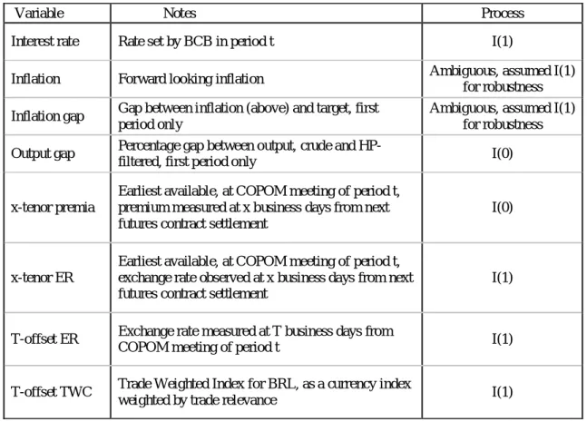
Table 10 below summarizes the findings. Inflation and inflation gap will be dealt with onwards as if I(1), to ensure a thorough study. T-offset TWC series will also be assumed I(1), though results aren't perfectly comparable. As mentioned previously, the TWC series has 157 observations, against 164 of other series.

Interest rate being I(1), though found also in the aforementioned works, is likely to be the most critical point. If it does not cointegrate with its regressors, this may produce spurious regressions.

(36)

Table 11 Summary of unit root tests.

Variable Notes Process

Interest rate Rate set by BCB in period t I(1)

Inflation Forward looking inflation Ambiguous, assumed I(1)

for robustness Inflation gap Gap between inflation (above) and target, first

period only

Ambiguous, assumed I(1) for robustness Output gap Percentage gap between output, crude and

HP-filtered, first period only I(0)

x-tenor premia

Earliest available, at COPOM meeting of period t, premium measured at x business days from next futures contract settlement

I(0)

x-tenor ER

Earliest available, at COPOM meeting of period t, exchange rate observed at x business days from next futures contract settlement

I(1)

T-offset ER Exchange rate measured at T business days from

COPOM meeting of period t I(1)

T-offset TWC Trade Weighted Index for BRL, as a currency index

weighted by trade relevance I(1)

3.4 Cointegration

Series that are I(1) in nature are required to cointegrate to avoid spurious regressions. For robustness, this criterion should exclude only output gap and x-tenor premia. The exchange rates series (x-tenor and T-offset) behave similarly and were grouped under “exchange rate series” for the purpose of this section.

Table 11 displays the results of the Johansen test for cointegration, both trace and maximum eigenvalue.

Table 12 Cointegration tests (trace test) for the below pairs.

Inflation Inflation gap Exchange rate

Interest rate None: 0.1565 None: 0.1003 None: 0.4281

One at most: 0.1361 One at most: 0.0513 One at most: 0.0814 Note: One and two asterisks (* and **) stand for rejections at 5% and 1% respectively.

(37)

Table 13 Cointegration tests (maximum eigenvalue test) for the below pairs.

One at most: 0.1361 One at most: 0.0513 One at most: 0.0814 Note: One and two asterisks (* and **) stand for rejections at 5% and 1% respectively.

A problem arises when there are signs that the COPOM-set short-term interest rate is not cointegrating with inflation gap and exchange rates, when the pairs are tested individually. This may indicate spurious regressions.

Inflation and inflation gap – following the same reasoning as on the previous section – will be tested for cointegration twice: one for the series used on this regression (above, the “original series”), and the other on the “clean series”, to validate or refute Taylor rule regressions done in the past. The 69-observations series were tested for cointegration and the results can be seen on the table below.

Table 14Cointegration tests (trace test) of the 69-observations series.

One at most: 0.0347* One at most: 0.0866 One at most: 0.1262 Note: One and two asterisks (* and **) stand for rejections at 5% and 1% respectively.

Table 15Cointegration tests (maximum eigenvalue test) of the 69-observations series.

One at most: 0.0347* One at most: 0.0866 One at most: 0.1262 Note: One and two asterisks (* and **) stand for rejections at 5% and 1% respectively.

This table produces results relevant to the validity of past regressions with Taylor rule in Brazil, in the analyzed period, with or without the exchange rate. The hypothesis of cointegration between inflation and interest rate was rejected at 5%, and the tests are bent towards no cointegration on the other two pairs as well (interest rate with inflation gap and interest rate with exchange rates).

The issue that arose with the mismatch in frequency of observations – between inflation and interest rates – proves to offer a trade-off. If the researcher uses the COPOM decisions on interest rates as its anchor for further analysis, the inflation series will be prohibitive for

(38)

error-correction models, for instance, as the first difference observations will be filled with zeroes in between values. On the other hand, if the researcher chooses to work with a “cleaner” inflation series, it will run into evidences of no cointegration. As a matter of fact, the very Johansen test with inflation and inflation gap, by the same reason described above, may be put to question given the correction term implied in its modelling. For that reason, as will be further explained, residuals will also be scrutinized in search of evidence of cointegration.

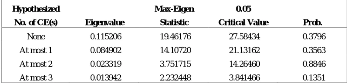
Finally, using the “cropped” series of inflation gap (no-null values during period 1 and null during period 2), cointegration between interest rates, inflation, inflation gap and exchange rate is not seen.

Table 16 Cointegration tests (trace test) for the base regression settings.

Hypothesized Trace 0.05

No. of CE(s) Eigenvalue Statistic Critical Value Prob.

None 0.115206 39.55312 47.85613 0.2389

At most 1 0.084902 20.09136 29.79707 0.4167 At most 2 0.023319 5.984163 15.49471 0.6974 At most 3 0.013942 2.232448 3.841466 0.1351 Note: One and two asterisks (* and **) stand for rejections at 5% and 1% respectively (none in this table).

Table 17 Cointegration tests (maximum eigenvalue test) for the base regression settings.

Hypothesized Max-Eigen 0.05

No. of CE(s) Eigenvalue Statistic Critical Value Prob.

None 0.115206 19.46176 27.58434 0.3796

At most 1 0.084902 14.10720 21.13162 0.3563 At most 2 0.023319 3.751715 14.26460 0.8846 At most 3 0.013942 2.232448 3.841466 0.1351 Note: One and two asterisks (* and **) stand for rejections at 5% and 1% respectively (none in this table).

The tests do not reject either cointegration nor no-cointegration. Table 17 summarizes the findings and updates the series that will be analyzed in section 4.5.

(39)

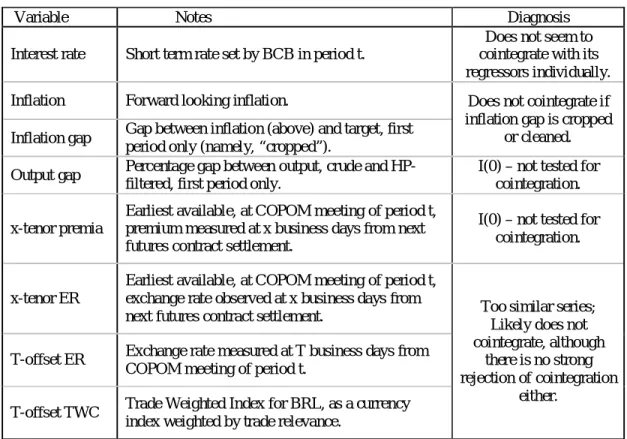
Table 18 Summary of cointegration analysis.

Variable Notes Diagnosis

Interest rate Short term rate set by BCB in period t.

Does not seem to cointegrate with its regressors individually.

Inflation Forward looking inflation. Does not cointegrate if

inflation gap is cropped or cleaned. Inflation gap Gap between inflation (above) and target, first

period only (namely, “cropped”).

Output gap Percentage gap between output, crude and HP-filtered, first period only.

I(0) – not tested for cointegration.

x-tenor premia

Earliest available, at COPOM meeting of period t, premium measured at x business days from next futures contract settlement.

I(0) – not tested for cointegration.

x-tenor ER

Earliest available, at COPOM meeting of period t, exchange rate observed at x business days from

next futures contract settlement. Too similar series; Likely does not cointegrate, although

there is no strong rejection of cointegration

either. T-offset ER Exchange rate measured at T business days from

COPOM meeting of period t.

T-offset TWC Trade Weighted Index for BRL, as a currency index weighted by trade relevance.

On a final note regarding mixed signals, the Johansen’s tests assume normality. Residual normality will be evaluated next, together with other indicators, to assess the goodness-of-fit. As an alternative to the Johansen tests (given the normality hypothesis and the VECM deterrent brought by the inflation series, as described earlier), the residuals of some regressions were tested for unit root. Residuals being I(0) are evidence of cointegration between the independent variable and its regressors. In the following chapter, where the results of the regressions are discussed, the residuals will be further detailed. In summary, neither of the regressions tested ended up producing I(1) residuals.