Regional Integration and Internal Economic Geography - an Empirical Evaluation with Portuguese Data

Regional Integration and Internal Economic Geography - an

Empirical Evaluation with Portuguese Data

Nuno Crespo

and Maria Paula Fontoura

(a) ISCTE-University Institute for Social Sciences, Business Studies and Technology,

Department of Economics, Av. das Forças Armadas, 1649-026 Lisboa, Portugal;

e-mail: nuno.crespo@iscte.pt

(b) ISEG/CISEP, Technical University of Lisbon, Rua Miguel Lúpi, 20,1200-781

Lisboa, Portugal; e-mail: fontoura@iseg.utl.pt

Author for Correspondence:

Maria Paula Fontoura

Rua Miguel Lúpi, 20

1200-781 Lisboa, Portugal

fontoura@iseg.utl.pt

1

The financial support provided by the Fundação para a Ciência e a Tecnologia under

Regional Integration and Internal Economic Geography - an

Empirical Evaluation with Portuguese Data

Abstract: The effects of the reduction of international trade costs on the internal economic geography of each country have been very scarcely studied in empirical

terms. With data for Portugal since its adhesion to the European Union, we test the

hypotheses put forward by the new economic geography concerning the evolution of

the spatial concentration of the manufacturing industry as a whole and of the different

industries individually considered. We consider alternative concentration concepts

and data disaggregated both at the level of NUTS III (28 regions) and concelhos

(275 regions). Results show a dispersion of total industry as a consequence of the

reduction of international trade costs, in line with Krugman and Elizondo (1996)’s

prediction. Individual industries show a similar tendency, in contrast with the

theoretical hypothesis.

Keywords: trade liberalization, industrial location, Portugal.

1. Introduction

Empirical work on the spatial dimension has attracted a vast interest in the last

fifteen years in the context of the so-called new economic geography (NEG). A large

number of studies on this topic have examined the impact of trade liberalization on

the location of economic activity within integrated spaces, with special emphasis on

the European Union (EU) case. Nevertheless, NEG also provides the adequate

conceptual framework to evaluate the impact of trade liberalization on the internal

economic geography of each member state. In particular, it allows to evaluate whether

economic integration leads either to internal structural convergence or to divergence,

thus contributing to the increase/decrease of internal economic cohesion.

Surprisingly, however, the empirical evidence on this internal spatial dimension is

very scarce and far from conclusive. Considering the Portuguese case, we aim to fill

this gap in the literature.

Relative to previous studies, we consider additional concepts of spatial

concentration and a wider set of indices as well as a much more disaggregated data at

the regional level. Furthermore, the database used covers the period since the

Portuguese adhesion to the EU (January 1986) and, therefore, it is particularly

adequate for the purpose of this paper.

The fact that Portugal is the EU member which depends most strongly on the EU

market (both with regard to exports and imports) gives a particular interest to this

country case.

The paper is organized as follows. In section 2, we present the theoretical

activity at the country level. In section 3, we analyze the results of the empirical

evidence previously produced on this question. In section 4, we describe the data and

discuss the different methodologies which will be used in the empirical evaluation of

the Portuguese case developed in section 5. Finally, in section 6, we present some

concluding remarks.

2. Theoretical guidelines

In a pioneering study on this topic, Krugman and Elizondo (1996) posit the

existence of a positive relationship between international trade costs and the degree of

spatial concentration of manufacturing industry as a whole.2 Inspired by the Mexican case, their model explains the growth of the giant Third Model metropolis (as is the

case of Mexico City) as a consequence of strong forward and backward linkages that

emerge when manufacturing industry tries to serve a closed domestic market. With

trade liberalization, these linkages are weakened and there is an incentive to the

dispersion of economic activity within the country.

To formalize the above mentioned relation, Krugman and Elizondo (1996)

employ an NEG model comprising three regions: two internal ones, which we

designate as 1 and 2, and an external one, representing the rest of the world, which we

designate as 0. Models of economic geography always incorporate the tension

between a centripetal force that fosters spatial concentration and a centrifugal force

which encourages dispersion of economic activity. In this model, the centripetal force

is represented by backward and forward linkages and the centrifugal force is

2

expressed by congestion costs resulting from the dimension of the region, specifically

related to commuting costs and land rents.

Labor is perfectly mobile between 1 and 2, but not between these regions and 0

and, in each region, production takes place at a single central point. There are iceberg

transport costs both between the internal regions (which we designate as τ) and

between the latter and 0, the transport costs from any of these regions to 0 being equal

(η1,0 = η2,0). The two types of transport costs are distinct not only in their value but

also in their own nature. While τ represents the internal distance and the

infra-structures quality, as in Krugman (1996), η also includes trade barriers.

The impact of trade liberalization on the internal economic geography is

investigated by giving different values to η. If η is very high, there will not be

international trade and therefore, 0 does not affect the internal distribution of the

economic activity. In this case, firms tend to locate close to each other in order to

have an easier access to intermediate inputs. The increase in labor demand generates a

wage increase, thereby attracting more workers and augmenting the dimension of the

domestic market. This process makes this location more attractive to other firms

which want to locate nearer to the final demand. The agglomeration process will cease

when this positive effect is offset by the increase of congestion costs.

If η decreases significantly, the centripetal force becomes less important, because

as firms become more dependent on the external market, the advantage associated

with the proximity to final demand and to domestic suppliers of inputs becomes less

relevant. As a result, there is an incentive for firms to move away from the more

congested internal region (where the centrifugal force is stronger) to the other region,

Through numerical simulations, Krugman and Elizondo (1996) verify that with an

intermediate value for η there are several stable equilibria: a symmetric equilibrium in

which the manufacturing industry is evenly divided between the two domestic regions

or, alternatively, the concentration in one of the regions. However, when η is low

enough, the only stable equilibrium is the symmetric distribution.

The main conclusion of Krugman and Elizondo’s (1996) model is thus clear: it is expected that the trade liberalization process will lead to the dispersion of the total

industry within the country.3 We designate this hypothesis as [H1].

An alternative view is proposed, for instance, by Paluzie (2001).4 The main difference between the two models is the consideration of different centrifugal forces.

In Paluzie (2001), it is given by the pull of a dispersed rural market, as in the standard

model of Krugman (1991). Labor mobility between regions generates unequal

geography within a country and it is shown, through numerical simulations, that trade

liberalization reinforces this effect. In fact, while for a high value for η, the symmetric

distribution between the two domestic regions prevails as equilibrium, the

consideration of a low value for η leads to a core-periphery pattern, with all

manufacturing industry concentrated in just one region. Paluzie (2001)’s conclusion

is, therefore, opposite to that obtained by Krugman and Elizondo (1996): a reduction

of international trade costs causes the concentration of total industry. We designate

this hypothesis as [H1’].

Until now, we have focused on the effect of the reduction of international trade

costs on the location of total industry. However, the changing pattern of industrial

3

For a critical perspective on this theoretical approach, see Isserman (1996) and Henderson (1996).

4

See also Monfort and Nicolini (2000), Monfort and van Ypersele (2003), Crozet and

location may not be uniform across industries. Fujita et al. (1999, chapter 18) show

that trade liberalization may bring spatial clustering of particular industries and,

therefore, regional specialization. In their model, the main centripetal force is given

by backward and forward linkages while, more in line with the standard NEG model,

the centrifugal force arises from final consumer demand in each location.5 With the reduction of η, both forces are weakened. The openness to international trade leads

the domestic firms to use a higher proportion of imported intermediate inputs and to

sell a higher proportion of their own production in the foreign market and encourages

the consumers to include a higher proportion of imports in their consumption.

However, through numerical simulations, Fujita et al (1999) observe that the

centripetal force prevails and, therefore, the specialization level of the regions tends to

rise. We designate this hypothesis as [H2].

3. A brief survey of empirical evidence

The fact that contradictory theoretical predictions may be derived with regard to

the impact of international trade costs reduction on the internal economic geography

of the countries makes the role of empirical evaluation of this topic even more

relevant. This section surveys the (still scarce) evidence produced so far in this area.

The most comprehensive study in terms of number of countries covered is that of

Ades and Glaeser (1995). With a sample of 85 countries and data for 1970, 1975,

1980 and 1985, they verify that an increase of 10% of the trade share in GDP leads to

a reduction of 6% in the size of the largest city, whereas an increase of 1% in the ratio

of import duties to total imports implies an increase of almost 3% in the size of the

5

largest city. Nevertheless, Nitsch (2001, 2003) contested the robustness of this

negative relation. For instance, considering different proxies for the degree of spatial

concentration and the degree of openness, a causal link between openness and

concentration is no longer observed either with Ades and Glaeser’s (1995) database or

in the case of other periods and groups of countries.

Other studies have concentrated their analysis on a specific country. The Mexican

case has been one of the most profusely analyzed. The size of Mexico City, in

addition to the adhesion of Mexico to NAFTA, makes this case particularly

appropriate for the testing of the theoretical hypotheses of section 2. Results suggest

that the removal of trade barriers initiated in the mid-1980s have contributed to the

decentralization of Mexican industry away from Mexico City, as shown, for instance,

by Krugman and Hanson (1993) and Hanson (1998). More recently, Arias (2003)

confirmed the existence of a dispersion movement evaluated in terms of employment

and production. In fact, in terms of employment, the share of total industry located in

the three largest Mexican cities decreased from 56.4%, in 1975, to 45.0%, in 1985,

and 37.6%, in 1993. These results suggest, however, that the dispersion movement

was already visible between 1975 and 1985, increasing in the period 1985-1993,

which points to the need for additional explanation.

De Robertis (2001) has analyzed the Italian case. With employment data in the

period 1971-91 for 20 regions, the author confirms [H1]. Using De Robertis’ (2001)

data, we have calculated the absolute Gini index - designated below as G(A)- for total manufacturing industry, obtaining values of 0.632, in 1971, and 0.596, in 1991, thus

reinforcing the evidence of the decrease of the absolute spatial concentration.6

6

Some analysis on [H2] has also been conducted for several countries, but in

general it has not been possible to draw a clarifying conclusion. In a pioneering study

on this topic, Hanson (1998) analyzes the Mexican case but the evidence obtained is

mixed. In De Robertis’ (2001) study on Italy, results are contradictory, depending on

the industry analyzed, with the sharpest increase in geographical concentration

registered by the textile and clothing industries, whereas the transport sector shows

the most significant opposite tendency.

Paluzie et al. (2001) present some evidence for Spain between 1979 and 1992.

The results, however, do not provide a clear confirmation of [H2] in the case of the

Spanish NUTS III regions. In fact, only 16 of the 50 regions considered show an

increase of specialization while, in terms of sectoral location, only 13 of the 30 sectors

show an increase in their level of spatial concentration. Moreover, these changes are,

on average, very moderate.7

To sum up, the existing studies, including those which concentrate on the

European integration process, do not present straightforward evidence, thus

reinforcing the importance of additional research in this field.

4. Measurement and data

Aiming to test the hypotheses formulated in Section 2, we consider statistical

information for Portugal between 1985 and 2000. We use employment data at the

2-digit level of the Classificação das Actividades Económicas (CAE), revision 2, for

7

The evaluation considers the Gini index. Although it seems to be the relative index (see next section),

manufacturing industry (sectors 15 to 37).8 The data is from Quadros de Pessoal - Ministry of Employment.9 In spatial terms, Portugal (excluding Madeira and Azores) consists of 5 NUTS II, 28 NUTS III and 275 concelhos. The two highest levels of

disaggregation are used in this paper, aiming to test the robustness of the conclusions.

Let us denote10 by xji the employment in sector j (j = 1, 2, …, J) in region i (I = 1, 2,

…, I) with J = 23 and I = 28 (in the case of the evaluation based on NUTS III) or 275

(in the case of the analysis based on concelhos).11

Based on the information of matrix X, we calculate, as an intermediate step to

obtain spatial concentration indices, the matrix S, with generic element sji = xji/xj

where xj is the total employment in sector j. Thus, sji represents the share of region i in

the locational distribution of j. We can also obtain matrix V, with generic element vji

= xji/xi where xi represents total employment in i. vji is, therefore, the share of sector j

in the sectoral structure of i. V is, therefore, an intermediate step to obtain

specialization indices.

8

At this level of aggregation, this nomenclature is fully compatible with NACE-Eurostat.

9

Until 1994, the information is presented according to CAE - revision 1. Therefore, this information

was converted into revision 2, in accordance with the conversion table between the two nomenclatures.

In order to minimize the problems associated with the conversion, statistical information until 1994 is

initially considered at the highest level of disaggregation and then converted to the 2-digit level of

revision 2.

10

For the sake of simplicity, we omit the time notation.

11

Since 1999, there have been 278 concelhos. In order to assure compatibility, we affect the values of

xji of the three new concelhos to those of which ones they were previously part, taking the area as

weight. Only in one case is it necessary to follow this procedure. In the two other cases, each new

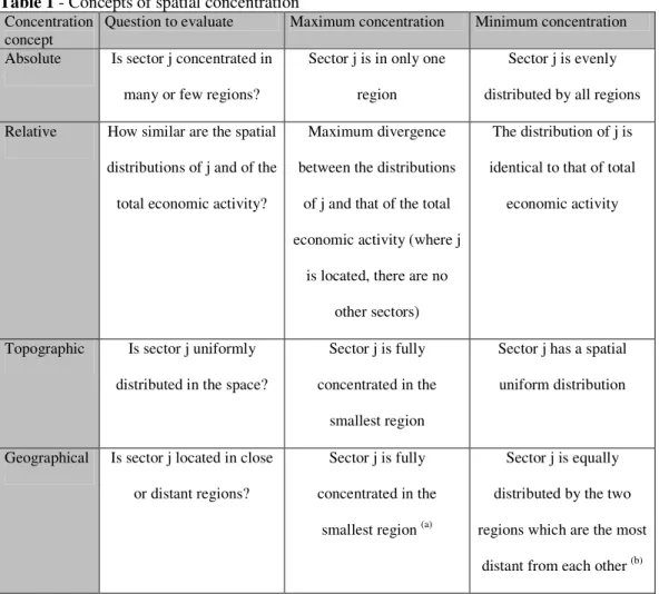
Aiming to obtain as comprehensive a vision as possible of industrial relocation

originated by the reduction of international trade costs, we use four alternative

concentration concepts: absolute, relative, topographic and geographical.

The concept of absolute spatial concentration only takes into consideration the

distribution of the sector in question by the different regions. Spatial concentration of

j will be the maximum when this sector is totally concentrated in only one region and

the minimum when it is distributed equally among all regions. We consider two

alternative indices of absolute concentration. The first is the commonly used Gini

index (Gj(A)). Its calculation implies the following procedure: (i) to rank the values of

sji in an increasing order, designating them by aj(h) with h (h = 1,2, …, I) indicating the

order; (ii) to obtain the partial accumulated values dj(h) such that dj(1) = aj(1), dj(2) = dj(1)

+ aj(2),…, dj(I) = dj(I-1) +aj(h); (iii) to define cj(h) = (h/I). The absolute Gini index is given

by:

I-1 I-1

G

= 1 - [ ( d

) / ( c

) ] ; G

[0 , 1]

[1]

Alternatively, we consider a new index which quantifies the deviations between

the effective locational distribution of j and a hypothetical equal distribution among

all regions. Taking the location coefficient as reference, it is expressed as follows:

I

E

= | s

- 1/I | ; E

[0, (2I - 2)/I]

[2]

i=1

Both indices increase with the degree of absolute concentration of the locational

In respect of the relative indices, they compare the locational distribution of j

with the distribution of a sector assumed as reference. As usually in these evaluations,

we use as reference “sector” the manufacturing industry as a whole (which we

designate as q) and, as such, we use this concept only in the evaluation of [H2]. The

first relative indicator used is the location coefficient, which can be expressed as:

I

E

=

β

| s

- s

| ; E

[0 , 2

β

[

[3]

In the most common case, β = ½ and, therefore, Ej ranges between 0 and 1, increasing

with the degree of dissimilarity between the two distributions considered.12

With regard to the relative Gini index it is obtained with the following procedure:

(i) considering the values of the location quotient (LQji = sji/sqi) and the corresponding

values of sji and sqi and ranking them in increasing order of LQji; (ii) designating the

values of LQji, sji and sqi ranked this way respectively by aj(h), bj(h) and eq(h) with h (h =

1, 2, …, I) representing the order; (iii) calculating the partial accumulated values gj(h)

such that gj(1) = bj(1), gj(2) = gj(1) + bj(2), …, gj(I) = gj(I-1) + bj(I); (iv) calculating the partial

accumulated values mq(h) such that mq(1) = eq(1), mq(2) = mq(1) + eq(2), …, mq(I) = mq(I-1)+

eq(I). The relative Gini index can be obtained as follows:

G

= 1 - [ ( g

) / ( m

) ] ; G

[0 , 1]

[4]

h=1 h=1

12

Gj(R) takes value 0 when the distribution of sji is equal to sqi and attains its maximum

value when j totally concentrates in only one region.

The two concentration concepts analyzed until now correspond to what is

commonly adopted in the empirical analysis. In the evaluation of absolute

concentration, all regions are considered as equal, whereas in the analysis of relative

concentration, the dimension of the regions has an economic character conferred by

the importance of the economic activity as a whole located in the different regions. A

complementary approach consists of considering the spatial dimension of the regions,

evaluated by their area.13 We designate this type of indicators as topographic indices. To evaluate the level of topographic concentration, we propose an approach

based on the adaptation of the relative indices.14 Let us define the area of i as ψi. We

calculate the share of the area of i in the total area, thus obtaining:

I

ϕi

=

ψi

/ (

ψi

)

[5]

i=1

The analysis of topographic concentration requires the comparison of the

locational structure of j with the one inherent to the values of ϕi. Using the location

coefficient as reference (with β = ½), the degree of topographic concentration of j can

be measured as follows:

13

The importance of this concept is greater if the dimensional dissimilarity between the regions is

significant. In the present case, the area of the Portuguese concelhos ranges from 7.97 Km2 (São João

da Madeira) to 1721.42 Km2 (Odemira).

14

TOP

= ½ | s

-

ϕi

| ; TOP

[0 , 1[

[6]

The minimum value of the admissible range corresponds to a uniform distribution of

j, i.e. when each region has a proportion of j equal to its share in terms of area.15 Any divergence facing this situation leads to an increase of topographic concentration.

Topj assumes its maximum value, converging to 1, when all the activity of j is located

in the smallest region.16

The indices that we have considered thus far ignore the geographical position of

the regions, i.e. they do not consider inter-regional distances. Nevertheless, it is also

important that the analysis of the locational concentration investigates if the

concentration occurs in nearby or distant regions. In order to control this factor,

Midelfart-Knarvik et al. (2000, 2002) propose an index of geographical separation.

However, this index does not consider the internal dimension of the regions, taking

the value 0 if j is fully concentrated in only one region, whatever it is. To overcome

this weakness, we propose an amplified version of this geographical index by

incorporating the intra-regional dimension. It is expressed as follows:

I K

GL

=

γ

(s

s

δik

) ; GL

]0 , +

∞

[

[7]

15

Obviously, a uniform intra-regional distribution is assumed. Therefore, the real topographic

concentration is sub-evaluated. The solution to this problem can only be attained by using very detailed

geographical information. The development of more sophisticated indices considering this type of

information is an interesting research topic. On this question, see Brülhart and Traeger (2003).

16

Topj never reaches 1 since that would mean that all the activity of j is located in a region with area

where γ is a constant17 and δik represents the distance between i and k.

Following Keeble et al. (1988) and Brülhart (2001), we use the expression δii =

1/3 (ψi /π)1/2 to calculate intra-regional distances.18 A rigorous use of this latter index

requires geographically detailed data. Therefore, we confine its application to the case

of the spatial dissagregation by concelhos. The calculation of GLj requires the

consideration of the bilateral distances between all the concelhos (75350

inter-regional and 275 intra-inter-regional distances). These distances are obtained from the

program ROUTE 66. We considered two ways of calculating distances: one in

kilometers - GL(km.) - and another which estimates the time (in minutes) needed to

travel that distance by car, taking into consideration the characteristics of thedifferent

roads (based on speeds pre-defined by the program) - GL(min.).

Table 1 summarizes the four concentration concepts used in this paper to evaluate

the level of locational concentration of a given sector j.

[Insert Table 1 here]

17

We assume γ=1.

18

As a result of an intense debate on this question, particularly in the context of the “border effects”

literature, there is, nowadays, a wide range of measures of intra-regional distances. For a survey on this

5. Empirical evidence for the Portuguese case

5.1. Evidence on total industry

As was observed in section 2, based on Krugman and Elizondo (1996), the

dispersion of the total manufacturing industry can be expected to take place as a

consequence of trade liberalization, with a reduction of the share of the total economic

activity located in the regions initially more congested. The opposite movement is

predicted, for instance, by Paluzie (2001).

A first way of evaluating this question consists of verifying whether the

locational structure of the total industry has changed significantly during the period

analyzed. With this objective, we use the Lawrence index which allows us to compare

the level of similarity of the locational structures of a given sector in two different

years. Designating it by Tj it is expressed as follows:

I

T

= ½ | s

- s

| ; T

[0 , 1]

[8]

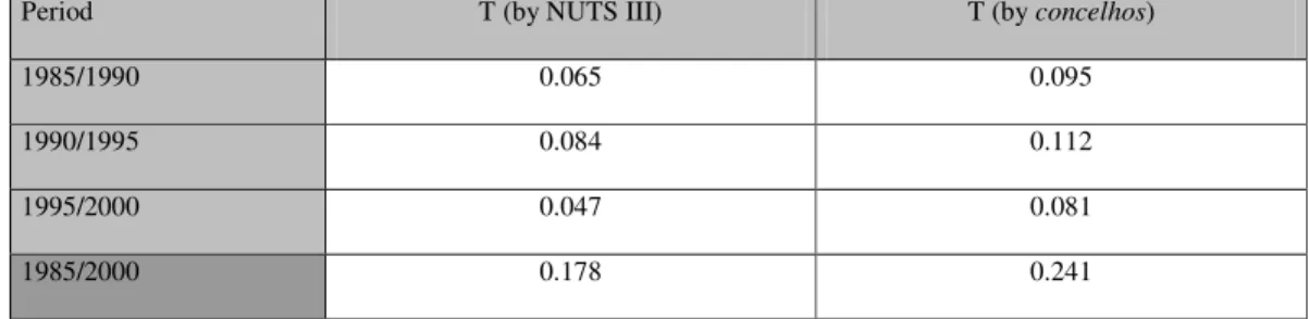
Tj ranges between 0 and 1, increasing with the transformation level of the locational

distribution of j. Table 2 presents the results concerning manufacturing industry as a

whole, between 1985 and 2000.

[Insert Table 2 here]

The evidence presented in Table 2 suggests a significant transformation in the

remarkable in the sub-period 1990-1995. In an annual evaluation, one verifies that it

is in the post-Single Market period that the locational transformation is the strongest,

particularly, by decreasing order, between 1995-1996, 1996-1997 and 1993-1994. The

replication of this analysis by concelhos points to a clear similitude of conclusions.

Once again, the transformation of the locational distribution is higher in the three

mentioned years.

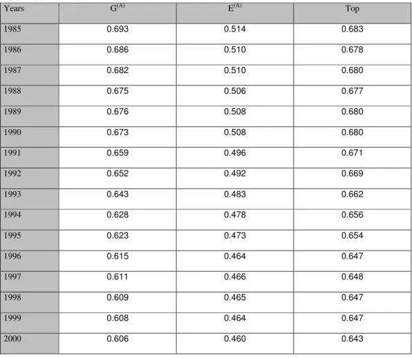
Using the indices presented in section 4, we focus now more specifically on the

evolution of the spatial concentration of total industry. Table 3 presents the results

based on a spatial disaggregation at NUTS III level. Note that in this case we only use

the absolute and the topographic indices since the geographical index requires

information at the concelhos level and the relative index is adequate only for

individual industries.

[Insert Table 3 here]

The evidence presented in Table 3 shows an evident decrease of absolute and

topographic concentration between 1985 and 2000. In fact, according to all the indices

considered, the maximum value is registered in 1985 and the minimum in 2000.

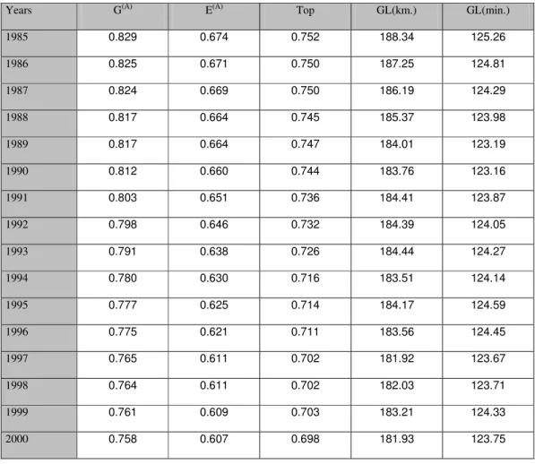
Turning now our attention to spatial disaggregation by concelhos, the results are

presented in Table 4.

[Insert Table 4 here]

The results obtained with the different indices at this level of spatial

the degree of absolute and topographic concentration of total industry. In its turn, the

analysis in terms of geographical concentration reveals a decrease of the geographical

separation between the regions where the industry is located. In fact, GL (min.)

decreases from 125,26, in 1985, to 123,75, in 2000.

A complementary picture to the previous results is provided in Table 5, which

presents the distribution of total manufacturing industry by NUTS III.

[Insert Table 5 here]

It is interesting to observe that the two regions with the highest share of total

manufacturing industry at the beginning of the period analyzed - Grande Lisboa (with

25.8%) and Grande Porto (with 19.4%) - register a very significant reduction of their

share, more accentuated in the case of Grande Lisboa, which shows the most

significant reduction among all the variations considered. Serra da Estrela, Península

de Setúbal, Algarve and Cova da Beira also have a reduction in the share of total

manufacturing industry located in those regions. Tâmega ((sqi00 - sqi85) = 0,0445),

Baixo Vouga and Cávado, all of them with a low share of total manufacturing

industry, display the most relevant increases of their shares. This general tendency is

confirmed by the correlation coefficient between sqi85 and (sqi00 - sqi85). The value

registered (- 0.752) reflects the reduction of the concentration in the initially more

congested regions.

The replication of this analysis at the level of concelhos shows that, in 1985, the

group of three concelhos with the highest proportion of manufacturing industry

comprises Lisboa (17.2%), Porto (5.6%) and Guimarães (5.2%). At the end of the

hierarchy, reflecting a strongly accentuated reduction of the relative weight of Lisboa

- which had only 3.9% of total industry in 2000 - and of Porto - with a share of 2.3%

in 2000. The correlation coefficient between sqi85 and (sqi00 - sqi85) at this spatial

disaggregation level is - 0.814, confirming the result previously presented.

The global conclusion which emerges from the evidence presented in this section

concerning the spatial distribution of total industry is a clear support for the

hypothesis postulated by Krugman and Elizondo (1996) - [H1]. In fact, during the

trade liberalization process that follows adhesion to the EU there is a clear dispersion

of total industry in the internal Portuguese space and a very significant reduction of

the share of manufacturing industry located in the initially more congested areas.

5.2. Evidence on individual industries

Having considered the evidence concerning the total industry, we focus now our

attention on the behavior of the individual sectors, in order to test the validity of [H2].

Once again, we start with the analysis of the transformation of the locational

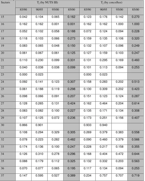
distribution by using Tj. The results obtained are presented in Table 6.

[Insert Table 6 here]

In what concerns the locational distribution at NUTS III level, a significant

transformation of the pattern of sectoral location is visible, mainly in sectors 27 (basic

metals) and 32 (radio, television and communication equipment). Sectors 17 (textiles)

and 18 (clothing) - which are predominant in the Portuguese economy - present

12th position in terms of spatial stability. In an evaluation by sub-periods, 14 sectors

have their highest locational transformation between 1990 and 1995.

The conclusions of the analysis at the concelhos level are similar to those for the

NUTS III with regard to the sectors with the sharpest locational transformation during

the period studied. However, in this case, it is also important to mention sector 34

(motor vehicles), besides sectors 16 (tobacco) and 37 (recycling), which present a low

weight in terms of total employment.

A relevant observation emerging from the results for Tj in annual terms, at both

levels of disaggregation, is that locational transformation is more accentuated in the

post-Single Market, suggesting that the results of other studies for the EU area which

do not include this period may be misleading.

Turning next to the analysis of the evolution of the degree of concentration of the

spatial structure of the different sectors, we use the indices proposed to represent the

four concepts of concentration considered.

In order to reduce the vast volume of information that is obtained with

calculations at the sectoral level, Table 7 indicates whether the sector registers a

concentration increase (+) or a concentration decrease (-) in the period analyzed. The

same purpose led us to select the commonly used Gini index (Gj(A)) to capture absolute

spatial concentration and the location coefficient (Ej) to express relative spatial

concentration.

The main result that emerges from Table 7 is an obvious divergence between the

conclusions derived, on the one hand, from the relative concentration index and, on

the other hand, from the absolute and topographic concentration indices.19

Let us observe that in the analysis by NUTS III, 13 sectors reveal an increase of

relative concentration (evaluated by Ej) while only 10 sectors show an opposite

tendency. In turn, the analysis based on the absolute index tells us that only sector 19

registered an increase of concentration during the period studied. The topographic

concentration index (Topj) corroborates this latter tendency as, according to this

index, only sectors 29 and 30 became more spatially concentrated.

This dichotomy of results is even more evident when we consider a

disaggregationby concelhos. In fact, the absolute and topographic indices indicate

that no sector increased its spatial concentration, whereas Ej signals an increase

tendency in 17 cases.

As a test of robustness, we have calculated the relative Gini index (Gj(R)) for the

two spatial levels that have been used. The results obtained show a high consistency

with the evidence generated by Ej.

How to explain the distinct message given by the different indices? A primary

explanation appears to be related to the fact that the use of relative indices

presupposes the stability of the region/sector taken as reference. Nevertheless, in the

present case, we have observed a strong transformation of the spatial distribution of

total manufacturing industry. Therefore, when the analysis for specific industries is

based on relative indices, the dispersion of total industry causes an increase of the

19

The interpretation of the geographical concentration index is more complex since its variation cannot

be unequivocally comparable with a specific evolution in terms of the remaining concentration

value of the index, which, in fact, is not related to a locational transformation of the

sector in question. Being so, it seems more appropriate to concentrate the evaluation

on the absolute and topographic indices, as the application of relative indices does not

seem to produce reliable conclusions whenever the spatial distribution of total

industry is not stable in the period analyzed.

The main conclusion to retain from the previous evidence is, therefore, a clear

rejection of the hypothesis formulated by the NEG literature with regard to individual

industries.

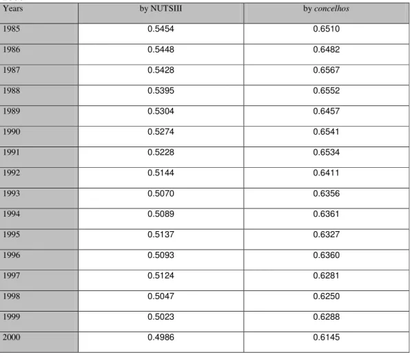
An alternative way of analyzing [H2] consists of evaluating the evolution of the

degree of similarity of the sectoral structures of the different regions. An increase of

specialization of the regions will be expressed in a growing divergence between their

sectoral structures. In order to evaluate this question, we calculate the specialization

coefficient in bilateral terms between all the pairs of regions for each year and for the

two levels of spatial disaggregation used. With the matrices containing this

information, we obtain, for each level of disaggregation, the simple averages in each

year, which give us an indication of the degree of similarity between the sectoral

structures of the regions. Table 8 presents the results.

[Insert Table 8 here]

Noting that a decrease of the value of the index signals a convergence of the

sectoral structures of the regions, the evidence presented in Table 8 clearly suggests

that, in the period analyzed, sectoral structures became more similar. This result is

(Cávado and Beira Interior Sul) and 66 concelhos display a movement of structural

divergence between 1985 and 2000, evaluated in average bilateral terms.

The evolution of the degree of average bilateral similarity for each region (i.e. of

that region compared with all the others) is, therefore, in line with the conclusion that

emerges from the indices of absolute and topographic concentration presented above.

One may thus conclude that the theoretical prediction of an increase of the degree

of specialization of the regions as a result of trade liberalization is not empirically

confirmed in the Portuguese case.

6. Final remarks

The empirical evaluation of the impact of trade liberalization on the internal

economic geography of each country is an important research topic which has been

widely neglected. However, NEG offers the appropriate conceptual framework to

study this question. The pioneering contribution of Krugman and Elizondo (1996)

presents a model where the reduction of international trade costs causes a dispersion

of manufacturing industry as a whole. However, other studies (for instance, Paluzie,

2001), making use of a distinct centrifugal force, reach an opposite conclusion.

Concerning individual industries, Fujita et al. (1999, chapter 18) predict a spatial

concentration movement and, therefore, an increase of the specialization level of the

regions.

Considering different concepts of concentration and data for Portugal between

1985 and 2000, we evaluate both predictions. The results concerning industry as a

whole confirm the hypothesis established by Krugman and Elizondo (1996), i.e. the

results differ according to the concentration concept adopted. Using the most

appropriate concepts for this specific analysis (i.e., the absolute and topographic

concentration), the results indicate the dispersion of the generality of the industries, in

References

Ades, A., and Glaeser, E. 1995. Trade and Circuses: Explaining Urban Giants.

Quarterly Journal of Economics 110: 195-227.

Arias, A. 2003. Trade Liberalization and Growth: Evidence from Mexican Cities. The

International Trade Journal 17(3): 253-273.

Brülhart, M. 2001. Evolving Geographical Concentration of European Manufacturing

Industries. Weltwirtschaftliches Archiv137(2): 215-243.

Brülhart, M., Crozet, M., and Koenig, P. 2004. Enlargement and the EU Periphery:

the Impact of Changing Market Potential. The World Economy 27(6): 853-875.

Brülhart, M., and Traeger, R. 2003. An Account of Geographic Concentration

Patterns in Europe. mimeo. University of Lausanne.

Chakravorty, S. 2003. Industrial Location in Post-Reform India: Patterns of

Inter-Regional Divergence and Intra-Inter-Regional Convergence. Journal of Development

Studies 40(2):120-152.

Crozet, M., and Soubeyran, P. 2004a. Trade Liberalization and the Internal

Geography of Countries. In Multinational Firms’ Location and The New Economic

Geography, ed T. Mayer and J. Mucchielli, 91-109. Cheltenham: Edward Elgar.

Crozet, M., and Soubeyran, P. 2004b. EU Enlargement and the Internal Geography of

De Robertis, G. 2001. European Integration and Internal Economic Geography: the

Case of the Italian Manufacturing Industry 1971-1991. The International Trade

Journal 15(3): 345-371.

Fujita, M., Krugman, P., and Venables, A. 1999. The Spatial Economy: Cities,

Regions and International Trade. Cambridge: MIT Press.

Hanson, G. 1998. Regional Adjustment to Trade Liberalization. Regional Science and

Urban Economics 28(4): 419-444.

Head, K., and Mayer, T. 2002. Illusory Border Effect: Distance Mismeasurement

Inflates Estimates of Home Bias. CEPII Working Paper No. 2002-01.

Henderson, J. 1996. Ways to Think About Urban Concentration: Neoclassical Urban

Systems Versus the New Economic Geography. International Regional Science

Review 19(1 and 2): 31-36.

Isserman, A. 1996. It’s Obvious, It’s Wrong, and Anyway They Said It Years Ago?

Paul Krugman on Large Cities. International Regional Science Review 19(1 and 2):

37-48.

Keeble, D., Offord, J., and Walker, S. 1988. Peripheral Regions in a Community of

Twelve Member States. Report for the European Commission, Brussels.

Krugman, P. 1991. Increasing Returns and Economic Geography. Journal of Political

Krugman, P. 1996. Urban Concentration: the Role of Increasing Returns and

Transport Costs. International Regional Science Review 19(1 and 2): 5-30.

Krugman, P., and Hanson, G. 1993. Mexico-U.S. Free Trade and the Location of

Production. In The Mexico-U.S. Free Trade Agreement, ed. P. Garber. Cambridge,

MA: MIT Press.

Krugman, P., and Elizondo, R. 1996. Trade Policy and the Third World Metropolis.

Journal of Development Economics 49: 137-150.

Midelfart-Knarvik, K., Overman, H., Redding, S., and Venables, A. 2000 The

Location of European Industry. The European Commission Directorate General for

Economic and Financial Affairs, Economic Papers No.142.

Midelfart-Knarvik, K., Overman, H., Redding, S., and Venables, A. 2002. Integration

and Industrial Specialisation in the European Union. Révue Économique 53(3):

469-481.

Monfort, P., and Nicolini, R. 2000. Regional Convergence and International

Integration. Journal of Urban Economics 48: 286-306.

Monfort, P., and van Ypersele, T. 2003. Integration, Regional Agglomeration and

International Trade. CEPR Discussion Paper No. 3752.

Nitsch, V. 2001. Openness and Urban Concentration in Europe, 1870-1990. HWWA

Nitsch, V. 2003. Trade Openness and Urban Concentration: New Evidence. Paper

presented at the European Trade Study Group Conference 2003, Madrid, 11-13

September.

Paluzie, E. 2001. Trade Policy and Regional Inequalities. Papers in RegionalScience

80: 67-85.

Paluzie, E., Pons, J., and Tirado, D. 2001. Regional Integration and Specialization

Table 1 - Concepts of spatial concentration Concentration

concept

Question to evaluate Maximum concentration Minimum concentration

Absolute Is sector j concentrated in

many or few regions?

Sector j is in only one

region

Sector j is evenly

distributed by all regions

Relative How similar are the spatial

distributions of j and of the

total economic activity?

Maximum divergence

between the distributions

of j and that of the total

economic activity (where j

is located, there are no

other sectors)

The distribution of j is

identical to that of total

economic activity

Topographic Is sector j uniformly

distributed in the space?

Sector j is fully

concentrated in the

smallest region

Sector j has a spatial

uniform distribution

Geographical Is sector j located in close

or distant regions?

Sector j is fully

concentrated in the

smallest region (a)

Sector j is equally

distributed by the two

regions which are the most

distant from each other (b)

Table 2 - Structural transformation of the locational distribution of total industry, 1985-2000

Period T (by NUTS III) T (by concelhos)

1985/1990 0.065 0.095

1990/1995 0.084 0.112

1995/2000 0.047 0.081

Table 3 - Level of locational concentration of total manufacturing industry by NUTS III, 1985-2000

Years G(A) E(A) Top

1985 0.693 0.514 0.683

1986 0.686 0.510 0.678

1987 0.682 0.510 0.680

1988 0.675 0.506 0.677

1989 0.676 0.508 0.680

1990 0.673 0.508 0.680

1991 0.659 0.496 0.671

1992 0.652 0.492 0.669

1993 0.643 0.483 0.662

1994 0.628 0.478 0.656

1995 0.623 0.473 0.654

1996 0.615 0.464 0.647

1997 0.611 0.466 0.648

1998 0.609 0.465 0.647

1999 0.608 0.464 0.647

Table 4 - Level of locational concentration of total manufacturing industry by concelhos, 1985-2000

Years G(A) E(A) Top GL(km.) GL(min.)

1985 0.829 0.674 0.752 188.34 125.26

1986 0.825 0.671 0.750 187.25 124.81

1987 0.824 0.669 0.750 186.19 124.29

1988 0.817 0.664 0.745 185.37 123.98

1989 0.817 0.664 0.747 184.01 123.19

1990 0.812 0.660 0.744 183.76 123.16

1991 0.803 0.651 0.736 184.41 123.87

1992 0.798 0.646 0.732 184.39 124.05

1993 0.791 0.638 0.726 184.44 124.27

1994 0.780 0.630 0.716 183.51 124.14

1995 0.777 0.625 0.714 184.17 124.59

1996 0.775 0.621 0.711 183.56 124.45

1997 0.765 0.611 0.702 181.92 123.67

1998 0.764 0.611 0.702 182.03 123.71

1999 0.761 0.609 0.703 183.21 124.33

Table 5 - Share of each region in the locational distribution of total manufacturing industry (si), 1985-2000

NUTS III 1985 1990 1995 2000

Minho-Lima 0.0106 0.0129 0.0177 0.0206

Cávado 0.0370 0.0489 0.0607 0.0619

Ave 0.1259 0.1351 0.1326 0.1355

Grande Porto 0.1935 0.1929 0.1584 0.1476

Tâmega 0.0397 0.0597 0.0725 0.0842

Entre Douro e Vouga 0.0607 0.0657 0.0726 0.0722

Douro 0.0028 0.0029 0.0039 0.0042

Alto-Trás-os-Montes 0.0035 0.0035 0.0040 0.0042

Baixo Vouga 0.0449 0.0494 0.0599 0.0712

Baixo Mondego 0.0211 0.0208 0.0218 0.0213

Pinhal Litoral 0.0290 0.0304 0.0342 0.0383

Pinhal Interior Norte 0.0076 0.0099 0.0117 0.0122

Dão Lafões 0.0112 0.0137 0.0175 0.0209

Pinhal Interior Sul 0.0017 0.0020 0.0025 0.0027

Serra da Estrela 0.0069 0.0048 0.0051 0.0037

Beira Interior Norte 0.0040 0.0046 0.0056 0.0063

Beira Interior Sul 0.0043 0.0052 0.0056 0.0052

Cova da Beira 0.0130 0.0129 0.0134 0.0121

Oeste 0.0271 0.0300 0.0353 0.0355

Grande Lisboa 0.2582 0.2050 0.1580 0.1322

Península de Setúbal 0.0398 0.0373 0.0440 0.0384

Médio Tejo 0.0199 0.0160 0.0222 0.0213

Lezíria do Tejo 0.0138 0.0140 0.0148 0.0176

Alentejo Litoral 0.0023 0.0025 0.0034 0.0031

Alto Alentejo 0.0050 0.0049 0.0056 0.0063

Alentejo Central 0.0054 0.0056 0.0070 0.0105

Baixo Alentejo 0.0018 0.0016 0.0021 0.0023

Table 6 - Transformation of the locational distribution of the manufacturing sectors (2 digit level), by NUTS III and concelhos, 1985-2000

Tj (by NUTS III) Tj (by concelhos)

Sectors

85/90 90/95 95/00 85/00 85/90 90/95 95/00 85/00

15 0.042 0.104 0.065 0.162 0.123 0.176 0.142 0.270

16 0.162 0.162 0.001 0.001 0.162 0.162 1.000 1.000

17 0.052 0.102 0.058 0.188 0.072 0.124 0.094 0.228

18 0.118 0.103 0.066 0.273 0.159 0.135 0.106 0.320

19 0.083 0.065 0.048 0.150 0.132 0.107 0.096 0.249

20 0.061 0.067 0.061 0.125 0.127 0.159 0.103 0.247

21 0.110 0.230 0.099 0.331 0.131 0.295 0.169 0.460

22 0.040 0.038 0.038 0.099 0.101 0.113 0.094 0.253

23 0.000 0.023 0.000 0.023

24 0.092 0.141 0.123 0.307 0.158 0.283 0.202 0.513

25 0.061 0.188 0.119 0.298 0.130 0.309 0.202 0.423

26 0.098 0.066 0.091 0.207 0.151 0.123 0.124 0.287

27 0.128 0.265 0.131 0.424 0.162 0.464 0.204 0.614

28 0.083 0.082 0.100 0.227 0.135 0.171 0.134 0.308

29 0.107 0.125 0.072 0.236 0.173 0.251 0.156 0.407

30 0.866 0.901 0.933 0.940

31 0.108 0.294 0.329 0.305 0.269 0.379 0.383 0.558

32 0.078 0.223 0.282 0.482 0.090 0.460 0.379 0.566

33 0.174 0.136 0.100 0.247 0.228 0.217 0.158 0.355

34 0.126 0.310 0.278 0.296 0.168 0.404 0.472 0.644

35 0.088 0.179 0.112 0.325 0.132 0.332 0.203 0.563

36 0.070 0.077 0.065 0.195 0.117 0.134 0.094 0.253

Table 7 - Evolution of the levels of concentration by NUTS III and concelhos, 1985-2000

by NUTS III by concelhos

Sectors

Gj(A) Ej Topj Gj(A) Ej Topj GLj (min.)

15 - + - - + - +

16 - + - - + - -

17 - - - - + - -

18 - + - - + - -

19 + - - - -

20 - - - -

21 - - - +

22 - + - - + - +

23(a) = + = = + = =

24 - - - - + - +

25 - - - -

26 - + - - + - +

27 - + - - + - +

28 - - - +

29 - + + - + - -

30(b) - + + - + - +

31 - - - - + - -

32 - + - - + - +

33 - - - - + - +

34 - + - - + - +

35 - + - - + - +

36 - + - - + - -

37 - - - +

Table 8 - Average bilateral similarity by NUTS III and by concelhos - global average, 1985-2000

Years by NUTSIII by concelhos

1985 0.5454 0.6510

1986 0.5448 0.6482

1987 0.5428 0.6567

1988 0.5395 0.6552

1989 0.5304 0.6457

1990 0.5274 0.6541

1991 0.5228 0.6534

1992 0.5144 0.6411

1993 0.5070 0.6356

1994 0.5089 0.6361

1995 0.5137 0.6327

1996 0.5093 0.6360

1997 0.5124 0.6281

1998 0.5047 0.6250

1999 0.5023 0.6288