DISSERTATION
A KERNEL MATCHING APPROACH FOR EYE DETECTION
IN SURVEILLANCE IMAGES
Diego Armando Benavides Vidal
Brasília, 23 November de 2016
UNIVERSIDADE DE BRASÍLIA
UNIVERSIDADE DE BRASILIA Faculdade de Tecnologia
DISSERTATION
A KERNEL MATCHING APPROACH FOR EYE DETECTION
IN SURVEILLANCE IMAGES
Diego Armando Benavides Vidal
Report submitted to the Department of Mechanical Engineering as a partial requirement for obtaining
the title of Master in Mechatronic Systems
Examination board
Díbio Leandro Borges, UnB
Advisor
José Maurício S. T. da Motta, UnB
Chair member
Hugo Vieira Neto, UTFPR
Benavides Vidal, Diego Armando
A kernel matching approach for eye detection in surveillance images / Diego Armando Benavides Vidal. –Brasil, 2016.
68 p.
Orientador: Díbio Leandro Borges
Dissertação (Mestrado) – Universidade de Brasília – UnB Faculdade de Tecnologia – FT
Programa de Pós-Graduação em Sistemas Mecatrônicos – PPMEC, 2016.
To
My life partner, Eloisa, for her support while I was following my passion, my madness. Thank you very much for being there.
Acknowledgments
Here, I am using the opportunity to express my sincere gratitude to each the persons that gave me their support through of these years. In the first place I want to thank my wife and my son to being there and support me everyday I love you so much. Also, I would also like to thank my parents for the support they provided me through my entire life. Thank Pedro and Olga, my success will always be their successes. In Brasilia, I would like to thank to my "cousin" Max Vizcarra who believed in me for achieve this challenge and received me in his house when I arrived in Brasília. Also, I would like to thank to my new family that I met the first year of the program, especially to my Colombian brother Sebastian. In fact with all of you I had feel as home. I have to say that the main experience also have been meet all of you and their cultures that despite being so different from mine, we could found some similar things about our brother countries.
I would like to thank to PPMEC for the opportunity that they got me and I sincere hope that the program achieve all of its targets. In general I have to thank to UnB and CAPES for opening me the door to a new universe so different to mine, in fact, was an adventure to know each aspects about the student and research life in Brasília.
Finally, I want to thank to the professors that were guide me through of program road including to Professor José Maurício Motta for his advices to start the dissertation, to profesor Li Weigang to complement my knowledge in the IA world and especially I would like to thank my advisor Díbio Borges for trust and interest in my work since the first email that I sent him and he will definitely does it until my defence. His teachings has strengthened my skills as researcher and I hope that we can work together participating in more conference, publications and projects in the future. I must emphasize the human side because there are few persons that look beyond their own interests. He could keep me in calm when the situation seemed into chaos. This was great help to achieve the goal. Thank very much Professor.
ABSTRACT
Eye detection is a open research problem to be solved efficiently by face detection and human surveillance systems. Features such as accuracy and computational cost are to be considered for a successful approach. We describe an integrated approach that takes the outputted ROI by a Viola and Jones detector, construct HOGs features on those and learn an special function to mapping these to a higher dimension space where the detection achieve a better accuracy. This mapping follows the efficient kernels match approach which was shown possible but had not been done for this problem before. Linear SVM is then used as classifier for eye detection using those mapped features. Extensive experiments are shown with different databases and the proposed method achieve higher accuracy with low added computational cost than Viola and Jones detector. The approach can also be extended to deal with other appearance models.
RESUMO
Table of Contents
Uma abordagem de funções kernel para detecção de olhos em imagens
de vigilância . . . ix
1 Introduction . . . 1
1.1 Presentation ... 1
1.2 Objectives ... 2
1.3 Structure of the document ... 2
2 Review of the literature . . . 4
2.1 Introduction ... 4
2.2 Eye detection based in Viola and Jones framework ... 4
2.3 Eye detection with different methods ... 6
2.4 Kernel methods for object recognition ... 10
2.4.1 Machine learning ... 11
2.4.2 Learning with kernel methods in object recognition ... 17
2.5 Summary ... 20
3 The proposed methodology . . . 21
3.1 Introduction ... 21
3.2 Eye detection problem in unconstrained settings ... 21
3.3 Viola and Jones detector as a first layer ... 22
3.4 EMK and SVM for eye detection ... 24
3.5 Efficient kernel eye detector design ... 26
3.6 Conclusion ... 31
4 Experiments . . . 34
4.1 Introduction ... 34
4.2 Datasets ... 34
4.3 Results and discussion ... 36
4.4 Conclusion ... 40
5 Conclusions . . . 44
5.1 Main contributions ... 44
5.3 Publications ... 45
Bibliography . . . 46
Anexos . . . 50
List of Figures
2.1 The Haar-like features ... 5
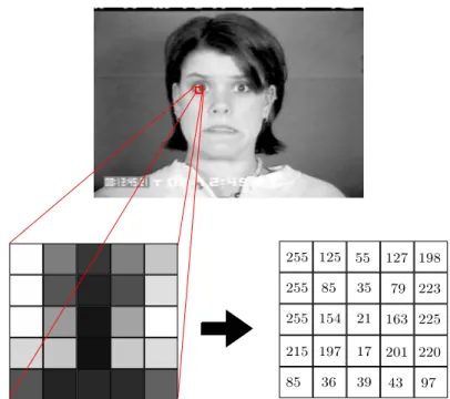
2.2 Example of calculating an integral image ... 6
2.3 Intensity pixel pattern in a ROI ... 7
2.4 Representation of a human in an image ... 8
2.5 Local variation of pixel in HOG ... 8
2.6 Racial differences. Shape and color. ... 10
2.7 Scene recognition using DPM’s and Latent SVM ... 10
2.8 Perceptron model present by Frank Rosenblatt... 11
2.9 Linearly separable training set ... 13
2.10 A geometric sample of maximum margin in SVM... 14
2.11 Kernel Trick representation in non-linearly separable input data setE... 16
2.12 Eye information on the image ... 18
3.1 A samples of CK+ database ... 22
3.2 A samples of FDDB database ... 23
3.3 Samples of resulting outputs of Viola and Jones detector. ... 24
3.4 Flow diagram of cascade classifier with Efficient Kernel Detector ... 24
3.5 Eye’s features design ... 25
3.6 HOG features samples using VJD outputs ... 26
3.7 Construction of HZ based on basis vector set ... 27
3.8 Extraction stage... 28
3.9 Training stage ... 31
3.10 Classification stage ... 33
4.1 Samples of the databases used in each stage of the proposed method. ... 35
4.2 Charts of the eye detector behavior by varying the among of basis vectors. ... 36
4.3 Charts of the eye detector behavior by varying λ. ... 37
4.4 Samples of false positives ROIs discarded by the proposed method. ... 37
4.5 Viola and Jones detector vs. EMK detector. ... 41
4.6 Viola and Jones detector vs. EMK detector. ... 42
List of Tables
2.1 Most common kernels used in the state-of-the-art ... 17
4.1 Precision obtained by Viola and Jones detector for each database. We used the implementation of VJD available in OpenCV Library with scale factor 1.05 and taking into account ROIs larger than 3×3. ... 38 4.2 Precision obtained by the proposed method compared with Viola and Jones results.
Nro. depicts the optimum value to amount of basis vector, λdepicts the optimum value to λand V&J represent the results obtained by Viola and Jones detector... 38 4.3 Results obtained in all of databases when the amount of the basis vector be varying.
List of Symbols
Symbols
R Region in a image
Ri The i-th rectangle in a image
P Patch or block defined as a subregion of a image
tp Normalized dimension of one size of a output generate for a detector
S Dimension of one size of a block. For example, a S×S block
p Size step using in the HOG feature structure
z Pixel of a image
c Amount of HOG features per block in a image
˜
m Magnitude of normalized gradient in a HOG framework
Gx Matrix of x axis variations in a HOG framework
Gy Matrix of y axis variations in a HOG framework
⌊a⌋ Major integer less than or equal to a used to characterized the descriptor vector of orientations per pixel z in a HOG framework
ǫp Small constant to avoids zero division
P Performance measure
Kp Kernel descriptor
P r Probability measure
K Integral operator
Kc Cluster number used in K-Means method
l The cardinality of a samples set
D The dimension of the mapping Φ(x)
Symbols Greek
λ Parameter in Gaussian kernel
∆ Variations between two values
Sets
R 1-dimensional Euclidean space Rn n-dimensional Euclidean space
H Hilbert space
E Samples set
T Tasks set
D Training set
D+ Training set samples labeled with y+ D− Training set samples labeled with y−
Y Labels set
Z Basis vector set
Funtions
i(x, y) Origin image function
ii(x, y) Integral image function
m(z) Magnitude function in HOG framework
θ(z) Orientation function in HOG framework
δ(z) HOG indicator vector
δi(z) HOG i-th bin of the indicator vector
ϑ(P) HOG feature vector for the patchP f Decision function
ˆ
f Decision function in Perceptron Model
g Linear function
ˆ
g Linear function in Perceptron Model
Φ Map function
k(x, y) Kernel function
Acronyms
2D Two dimensional
3D Three dimensional
MTC Modified Census Transform SVM Support Vector Machine HOG Histogram of oriented gradient DPM’s Deformable part-based models ERM Empirical risk minimization KKT Karush Kuhn Tucker BOW Bag of words
EMK Efficient match kernel
PCA Principal component analysis DP Dual program
ROI Region of interest
Uma abordagem de funções kernel para detecção
de olhos em imagens de vigilância
Capítulo 1: Introdução
A detecção ocular vem sendo uma parte importante no desenvolvimento de sistemas de detecção pessoal e de ações do corpo humano em geral. É muito comum em áreas de aplicação assim como segurança por imagens e interação entre humano e computador, os quais frequentemente requerem alta precisão, exatidão e velocidade. Uma resposta rápida e precisa é a preocupação principal das pessoas em segurança visual, e a detecção ocular pode ser considerada a primeira e uma parte essencial de qualquer sistema de segurança facial e também para aplicações de rastreamento ou identificação [Yang, Kriegman e Ahuja 2002].
São muitos os desafios que devem ser citados quando lidamos com problemas de detecção ocular em sistemas de segurança de vídeo. Desafios como deformação, ponto de vista, estruturas variáveis e oclusão são os mais frequentemente achados no contexto de segurança por vídeo porque isso é feito num ambiente não controlado. Nesse sentido, sistemas de segurança atuais devem ser capazes de lidar com esses desafios sem um impacto significante em sua performance.
Muitos trabalhos [Awais, Badruddin e Drieberg 2013, Chen et al. 2014, Choi, Han e Kim 2011, Hyunjun, Jinsu e Jaihie 2014, Oliveira et al. 2012] que são feitos com a melhor tecnologia possível citaram os problemas com a detecção ocular, os quais obtiveram resultados em pesquisas conhecidas. Uma das abordagens mais influentes para a detecção ocular foi proposta por Viola e Jones no [Viola e Jones 2004]: Eles propuseram um método que incluía a ideia da imagem integral para computar características Haar-like em várias escalas diferentes para descrever uma imagem, e um algoritmo de apredizagem AdaBoost para seleção e classificação das características. Embora principalmente usado para detecção facial baseado em partes da face assim como nariz, boca e olhos, a abordagem de Viola e Jones é útil para a detecção de vários objetos como carros e pedestres por exemplo. Pesquisas tem se baseado no [Viola e Jones 2004] para gerar sistemas de detecção melhores em tempo real. Isso ocorre pela velocidade de resposta e o baixo custo computacional. De qualquer modo, as características Haar-like para detecção em ambientes não controlados geram um grande número de falsos positivos, portanto outros métodos devem ser usados para melhorar seu resultados.
também podem ser usados para resolver o problema de dados não linearmente separáveis num espaço de entrada mais complexo. Assim, poderemos obter um detector ocular com melhor precisão sem um aumento considerável do custo computacional. Resultados experimentais obtidos usando os conjuntos de dados FDDB [Jain e Learned-Miller 2010], BioID [Jesorsky e Kirchberg Klaus e Frischholz 2001, CK+ [Lucey et al. 2010] e FERET [Phillips et al. 2000] mostram que nosso método alcança uma melhor precisão.
Capítulo 2: Revisão da literatura
Este capítulo familiariza o leitor com os trabalhos mais importantes citando os problemas da detecção ocular em imagens coletadas em ambientes espontâneos e como os métodos kernel são usados no reconhecimento visual. Existem trabalhos fora do contexto de segurança que precisamos mencionar, portanto dividimos esse capítulo em três partes importantes. A detecção ocular baseada na estrutura de Viola e Jones, a detecção ocular com diferentes métodos e detecção de objetos com os métodos kernel.
A seção 2.2 resume a estrutura Viola e Jones e os métodos baseados nela. A seção 2.3 apresenta os trabalhos mais importantes fora da estrutura Viola e Jones. Finalmente, a seção 2.4 apresenta um breve resumo das principais noções sobre os métodos Kernel que foram usados na detecção de objetos.
Capítulo 3: A metodologia proposta
Capítulo 4: Experimentos
Neste capítulo nós descrevemos os resultados obtidos pelo detector proposto nesse trabalho. Primeiro, é detalhado os bancos de dados usados para os testes e os parâmetros para usar em cada caso. Nós apresentamos dois tipos de experimentos. O primeiro está relacionado com a quantidade de vetores base usado para definir as características de um olho. O objetivo deste experimento é validar se há melhorias nos resultados quando a quantidade de características de base aumenta ou diminui. O segundo experimento está relacionado com o parâmetro λdo Kernel Gaussiano usado para construir os descritores Kernel. É recomendado analisar os resultados do detector proposto quanto este parâmetro muda porque não existe um valor padrão para garantir que os resultados para um determinado problema serão os melhores. É informado anteriormente que os resultados de saída obtidos pelo detector Viola e Jones serão utilizados para comparações.
A seção 4.2 detalha todos os bancos de dados a se usar. Na seção 4.3 nós explicamos os resultados obtidos pelo detector proposto destacando dois tipos de testes em particular, quando a quantidade de vetores base muda e quando o valor do parâmetro λmuda.
Capítulo 5: Conclusões
Nós descrevemos um método de detecção ocular que trabalha com configurações sem restrições e melhora a detecção em vários bancos de dados de imagens. Uma aproximação de um mapea-mento foi construída baseada em características HOG num subespaço de Hilbert provendo novas características conhecidas como descritores kernel eficientes [Bo e Sminchisescu 2009].
O detector de olho melhora os resultados do conhecido detector Viola e Jones usando os de-scritores kernel de características locais, com pelo menos 19% (FERET dvd1) mais precisão no pior caso, e 47% no melhor caso (CK+).
Esses descritores são projeções de vetores de características mapeados num espaço Hilbert de alta dimensão e são construídos baseados num conjunto finito de vetores base e operações com um kernel Gaussiano. Nós construímos esses descritores kernel para melhorar os resultados obtidos pelo detector Viola e Jones para olhos e obtivemos uma redução significativa em falsos positivos sem uma redução relevante dos verdadeiros positivos. Isso mostra que as características kernel levam em conta características de baixo nível que complementam a cada uma onde se detecta através da estrutura Viola e Jones sem custo adicional computacional durante todo processo de detecção. Como nós focamos apenas no resultado do detector Viola e Jones, as regiões de interesse foram reduzidas. Isso reduz o espectro de características falhas encontradas na projeção de um olho numa imagem.
Chapter 1
Introduction
1.1
Presentation
Eye detection has been a major part in the development of people detection systems and actions of the human body in general. It is very common in application areas such as security, video surveillance and human-computer interaction, which often require high precision, accuracy and speed. A fast and precise response is a major concern in visual surveillance of people, and eye detection can be considered a first and an essential part of any face surveillance system, either for tracking or for identification applications [Yang, Kriegman and Ahuja 2002].
Many are the challenges that must be addressed when we deal with eye detection problem in video surveillance applications. Challenges as deformation, viewpoint, variable structure and occlusion are most often found in context of video surveillance because in that is treated with uncontrolled environments. In that sense, current surveillance systems must be able to deal with them without significantly impacting its performance.
Many works [Awais, Badruddin and Drieberg 2013, Chen et al. 2014, Choi, Han and Kim 2011, Hyunjun, Jinsu and Jaihie 2014, Oliveira et al. 2012] inside state of the art have addressed the problem of eye detection which have resulted in well known investigations. One of the most influential approaches for eye detection was proposed by Viola and Jones in [Viola and Jones 2004]. They proposed a method including the idea of an integral image to compute Haar-like features in many different scales to describe an image, and an AdaBoost learning algorithm for features selection and classification. Although mainly used for face detection, and based on parts of faces such as nose, mouth and eyes, Viola and Jones approach is useful for many object detection tasks such as cars and pedestrians for example. Researchers have been based in Viola and Jones work to generate better detection systems. That is because its fast responses and low computational cost. However, Haar-like features for detections in uncontrolled environments generate a large number of false positives so other methods should be used.
between points. A multi-view manifold regularization learning and hypergraph matching was pre-sented in [Hong et al. 2015] for 3D generic object recognition from 2D images with state of the art results.
Here, we propose a method to address the eye detection problem by combining the outputs of a Viola and Jones detector (VJD) and improving its precision in an efficient match kernel framework. A particular set of features are derived over the outputs of the Viola and Jones detector and an algorithm for learning and classifying those in a kernel matching paradigm is described and tested. Efficient kernel descriptors were proposed in [Bo and Sminchisescu 2009] as a general tool for visual recognition. Here, in order to reduce the amount of false positives of the Viola and Jones detector without significantly reduce the amount of true positives, we used the efficient kernel framework to construct a new class of features based on HOG (Histogram of oriented gradient) features and train a linear SVM (Support Vector Machine) using two class, eye or non-eye. The main contribution of our work is to show that these descriptors can also be used to solve the non linearly separable problem in a challenging input space. Thus, we can obtain an eye detector with better accuracy without significantly increase of the computational cost. Experimental results obtained using FDDB [Jain and Learned-Miller 2010], BioID [Jesorsky, Kirchberg and Frischholz 2001], CK+ [Lucey et al. 2010] and FERET datasets [Phillips et al. 2000] show that our method achieve the state of the art accuracy.
1.2
Objectives
The main objective of this work is to design, construct and test an efficient eye detector in environments not controlled. It is desired that this detector has fast responses and be able to confront the usual challenges of detection.
The specific objectives of this work are listed below:
1. Show that the kernel descriptors are a good complement to the Haar-like features.
2. Construct an algorithm to extract and train kernel features for eye detection.
3. Construct an application to test the proposed eye detector.
4. Test the proposed detector with known databases and generate indicators that show that the results obtained by Viola and Jones detector are improved significantly.
5. Validate that the kernel descriptors are an elegant way to address the challenges present in eye detection.
1.3
Structure of the document
Chapter 2
Review of the literature
2.1
Introduction
This chapter familiarizes the reader with the most important works addressing the eye detection problem on images in unconstrained environments and how the kernel methods are used in visual recognition. There are important works outside of the surveillance context that we need to mention, so we divided this chapter in three main parts. Eye detection based in the Viola and Jones framework, eye detection with different methods and object detection using kernel methods.
Section 2.2 summarizes the Viola and Jones framework and the methods based on it. Section 2.3 present the most important works whose do not use the Viola and Jones framework. Finally, Section 2.4 present a brief review of the main notions about kernel methods that have been used in object detection.
2.2
Eye detection based in Viola and Jones framework
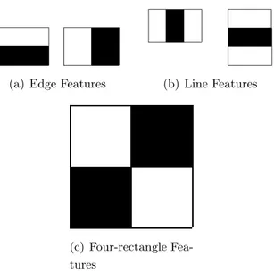
(a) Edge Features (b) Line Features
(c) Four-rectangle Fea-tures
Figure 2.1: The Haar-like features used in Viola and Jones framework and the same features are used in many current investigations.
ii(x, y) = X
x′≤x,y′≤y
i(x′, y′), (2.1)
whereii(x, y) is the integral image andi(x, y) is the original image.
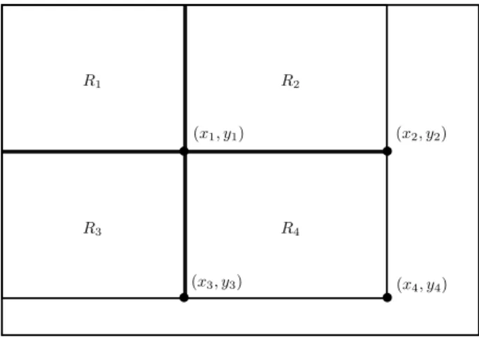
Figure 2.2 shows how the integral image works to calculate the rectangle pixel sum. If we need the pixels sum of the rectangle R4 only the operationii(x4, y4) +ii(x1, y1)−(ii(x2, y2) +ii(x3, y3))
is required.
The integral image is a strong contribution but a second contribution was made. A classi-fier by the selection of critical visual features through an AdaBoost learning algorithm [Freund and Schapire 1997] was constructed to improve de classification rate. More about this cascade architecture is explained in the Chapter 3 for our proposed method.
Many researchers have been follow the work of Viola and Jones [Awais, Badruddin and Drieberg 2013, Chen et al. 2014, Choi, Han and Kim 2011, Hyunjun, Jinsu and Jaihie 2014, Oliveira et al. 2012]. For instance, a boosting classification using Haar-like features was used to detect faces and eyes in [Chen et al. 2014] for real-time eye detection and identifying events. Similar strategies to reduce the computational cost of the detection were used in [Awais, Badruddin and Drieberg 2013] for detecting both eyes. Based on the correct face detection, a golden ratio was used to detect the eye pair in that work. By first detecting one eye and then applying symmetry of the face, the other eye could be detected. Then this detection was used to track the eye blinking. Also, in [Choi, Han and Kim 2011], AdaBoost approach was used with Modified Census Transform (MCT) [Froba and Ernst 2004] to construct a linear combination of weak classifiers with MCT-based eye features for eyes blinking detector.
b b
b
b
(x1, y1) (x2, y2)
(x3, y3) (x4, y4)
R1 R2
R3 R4
Figure 2.2: Calculation of rectangle sum using four array reference. (x1, y1),(x2, y2),(x3, y3) and
(x4, y4) are the reference in the original image andR1,R2,R3 and R4 are regions in the original
image.
locate features over regions of interest. Features as are shown in Figure 2.3 were found in the resulting outputs of Viola and Jones detector and with these was built an algorithm used in a cascade classification to decrease the number of false positives.
All the works detailed in this section have a good speed ratio as their better characteristic but the accuracy for eye detection in complex environments could still be improved. In Section 2.3 we will review another types of methods that focusing in the precision instead of speed.
2.3
Eye detection with different methods
The major contribution of the methods referred in Section 2.2 is their ability to perform the detection with an acceptable speed for real-time applications. However, their major disadvantage is that they do not have a good precision in uncontrolled environments and sometimes in controlled environments too. Taking into account that for a good detection in surveillance context accuracy is an important feature, it is necessary make a review to the methods focusing in optimize that feature in the state of the art even leaving aside the detection speed.
Figure 2.3: Intensity pixel pattern in eye image on middle row of pixels and the graph of intensity of many eye samples.
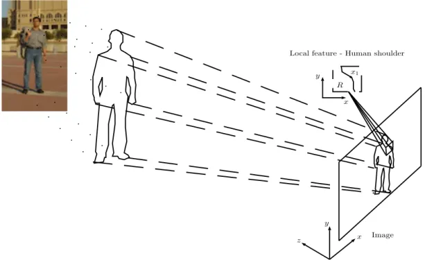
possible find a way to extract human features in an image as shown in Figure 2.4. The human shoulder in Figure 2.4 has some patterns in the image which can be expressed with variations of the pixels intensity. This variations can be used to construct a features vector or descriptor vector to train a classifier.
Formally, Histogram of Oriented Gradients or HOG is a model for extraction of low level features. Basically, it consists in build a histogram of magnitudes m(z) and orientations θ(z)
of variation vectors of each pixel z of image. This construction is done within of a set-patch of sub-regions of the image or ROI (Region of interest). Given that in image processing an image is considered a scalar matrix (e.g, image in grayscale) where each scalar represent a pixel, we can calculate the variation of each pixel in two directions using the rows and columns of the matrix. For example, givenzpixel inside3×3image as shown in Figure 2.5. The resulting variation vector consist in the variations in the axis x and y of the neighbors pixels close to z, that is, in axis x there would be a variation of ∆x = 94−54 = 40 and in axis y, ∆y = 101−45 = 56. So, the variation vector for the pixel z is(∆x,∆y) = (40,56). Repeating this process for all the pixels at the image patch, two matrixGx andGy are obtained. Those contains the variations in axesxand
y
x z
Local feature - Human shoulder
y
x R
b
x1
Image
Figure 2.4: Representation of a human in the image. HereR is the area of a local features.
94
54
101
45
32
88
66
79
z
y
x
Figure 2.5: Local variation of pixel at 3×3image on the construct of HOG descriptors.
After calculating the matrixGx andGy is straightforward to get magnitudem(z) and orienta-tion θ(z) of the resulting gradient vector for each pixelz in an image using the equations
m(z) =qG2
x(z) +G2y(z), (2.2)
θ(z) = arctan
Gy(z)
Gx(z)
, (2.3)
where Gx(z) yGy(z) represent the variations of pixelz in axisx and y respectively.
the intensity variation expressed as orientation of each pixel is discretized into a d-dimensional indicator vector δ(z) = [δ1(z),· · · , δd(z)]with
δi(z) =
(
1, ⌊dθπ(z)⌋=i−1
0, otherwise. (2.4)
wherei= 1,· · ·, dand⌊a⌋takes the major integer less than or equal toa. Therefore, the resulting vector descriptor of orientations for a pixelz, taking into accountdbins, isδ(z) = [δ1(z),· · ·, δd(z)]. Now, as we already have a categorization of orientations and we can calculate the magnitudesm(z)
for each pixel z, it is possible build the features vector of the form ϑp(z) =m(z)δ(z). Adding this idea in a image patch P (or ROI) we obtain the histogram of oriented gradients (HOG)
ϑ(P) =X
z∈P
˜
m(z)δ(z) (2.5)
where m˜(z) =m(z)/pP
z∈Pm(z)2+ǫp is the magnitude of normalized gradient, withǫp a small constant that avoids zero division.
The functional relationship (2.4) that induces the bins is a strong expression of the underlying classification that was taken for the simple presentation of the problem. For practical purposes, it is common to use a soft expression as is used in [Bo and Sminchisescu 2009].
Many works have been inspired by [Dalal and Triggs 2005] but the most important work for object detection that deals with the problem of accuracy was developed in [Felzenszwalb et al. 2010]. Even though it was not necessarily developed for eye detection but for objects as cars or persons, that approach can be adapted for objects detection in general. In that work the authors focused in many challenges that appear in the problem of object detection. For instance, many variations arise in illumination and viewpoint as in the case of eye detection in unconstrained environments, but they are not necessarily unique variations. There are non-rigid deformations, and intraclass variability in shape and other visual properties too. A sample of this can be seen when we look within different classes of races that exists between people in the world. For example, Asian people have a different eye shape than people of south America as shown Figure 2.6. To address these challenges in [Felzenszwalb et al. 2010] was proposed an object detection system that represents highly variable objects using mixtures of multi-scale deformable part models. This system is based on the framework extension of the pictorial structures [Fischler and Elschlager 1973], [Felzenszwalb and Huttenlocher 2005] using visual grammars [Felzenszwalb and McAllester 2007], [Jin and Geman 2006], [Zhu and Mumfordt 2007] to represent objects with variable hierarchical structures called deformable part-based models or DPM’s. In addition, and because of the nature of grammar based models, it is necessary use a latent variable formulation called latent SVM [Yu and Joachims 2009]. It is because that object representation is composed of unlabeled parts (sub-regions of the image) of the object of interest such that this information must be considered as latent information.
(a) Asian people. (b) South American people.
Figure 2.6: Racial differences. Shape and color.
based in two types of filter in multiple scales. Based in the HOG features used in [Dalal and Triggs 2005] a response through a root filter plus part filters is calculated to make a match. Using that match approach is possible obtain the localization of root box that contain the object of interest and its parts. Later, these box and part boxes are used to construct a total feature to training a latent SVM.
The same approach was used in [Pandey and Lazebnik 2011] to scene recognition as shown Figure 2.7. In that work the authors demonstrated that DPM’s are capable to recognize disordered structures taking into account latent variable for the training.
Figure 2.7: A sample of scene recognition made in [Pandey and Lazebnik 2011]. Left column: root and part filters based HOG features. Right five columns: root and parts box position of the scene.
2.4
Kernel methods for object recognition
recognition.
2.4.1 Machine learning
Learning is a word difficult to define and it is possible to find a different definition about that in many research areas as Psychology, Neuroscience, Medicine, Computer Science or Mathematics. In this section we do not have as a target finding a correct definition about learning but explain existing models about machine learning that are known inside the area of artificial intelligence. In this sense, it is presented below a machine learning definition made by Tom Mitchell in his book [Mitchell 1997] that will be used along this work.
Definition 2.4.1 (Machine learning) A computer program is said to learn from experience E
with respect to some class of tasksT and performance measure P, if its performance at tasks inT, as measured by P, improves with experienceE.
To understand this definition we can use the context of eye detection and settingT as recogniz-ing and classifyrecogniz-ing eye images, P as percent of eyes correctly classified andE as database of eyes with given classifications. Throughout this work is considered T as a tasks set,E as a samples set and P as a performance measure.
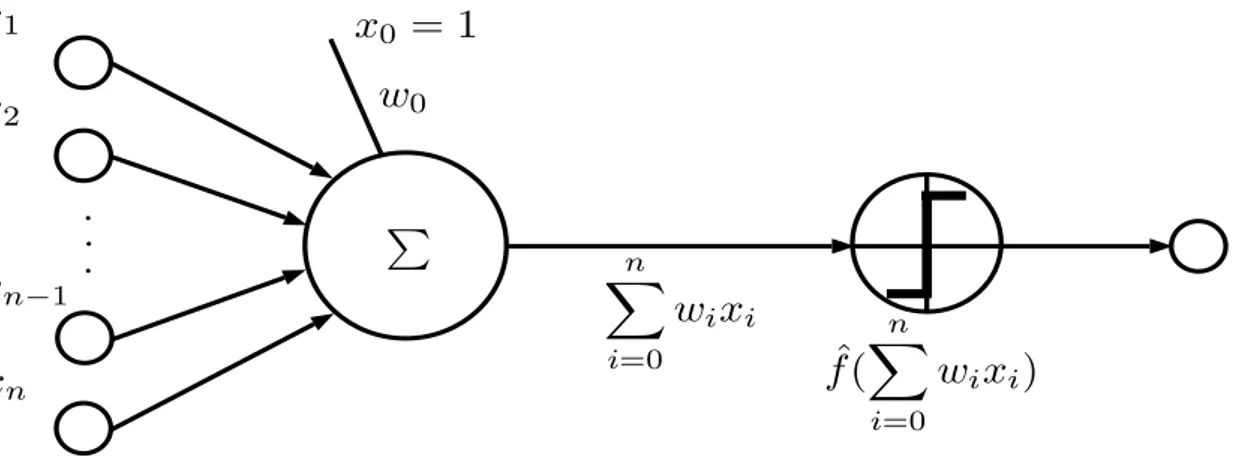
A model about machine learning made according Definition 2.4.1 was the Perceptron model by Frank Rosenblantt in [Rosenblatt 1958]. It was presented as a hypothetical nervous system designed to mimic some of the organized systems of the brain for human learning. Many researches about object recognition has been inspired in Rosenblatt’s work so it is good explain main keys about it.
x
1x
2x
n−1x
nP
.
.
.
x
0= 1
w
0n
X
i=0
w
ix
iˆ
f
(
n
X
i=0
w
ix
i)
Figure 2.8: Perceptron model present by Frank Rosenblatt in 1958. Here x1, x2, · · ·, xn are
components of a vector that represent a sample of data in E. This vector is used to estimate weight parameters wi in a linear function. Then, this function is used to calculate an output response fˆ(·) usually called decision function.
So according to Definition 2.4.1 suppose we have a set of samples E ⊂ Rn where ~xm =
(xm1,· · ·, xmn)is a sample, and a set of labels Y ={y−, y+} ⊂Rthat we can associate with each
D={(~xm, ym) :~xm ∈E∧ym ∈Y}. (2.6)
Rosenblantt proposed a learning model where is build a linear function gˆsuch that
ˆ
g(~xm) = n
X
i=0
wixi, (2.7)
where ~xm ∈ E, x0 = 1 and {w0,· · ·w1} ⊂ R is a weight set which should be calculated through
an iterative algorithm based on E in a process called training. This is made by a performance measure P such that
P(~xm) =||fˆ( n
X
i=0
wixi)−ym||, (2.8)
where ym is the label associated with the sample ~xm and fˆ: Rn → Y ⊂ R is a function that return the estimated label for sample ~xm called decision function. Here, P allow us to estimate the correct amounts of each element in {wi} using E for a given T. Figure 2.8 shown this basic learning model.
The approach made by Frank Rosenblatt inspired models such as classical neural networks and more elegant models as SVM. In this work we are interested in explain more about SVM because it is used as learning method for the proposed eye detection system. But first, it is necessary translate the idea of the perceptron approach as a binary classification problem.
The binary classification problem is defined as the task of distributing the elements of a not empty training set D such thatD=D+∪D− and D+∩D−=∅ where
D+={(~xm, ym) :ym=y+} and
D−={(~xm, ym) :ym=y−}.
(2.9)
In practice is possible to perform this type of classification through a function g : Rn → R but
that is not always easy. A basic sample can be shown if a training set D is linearly separable.
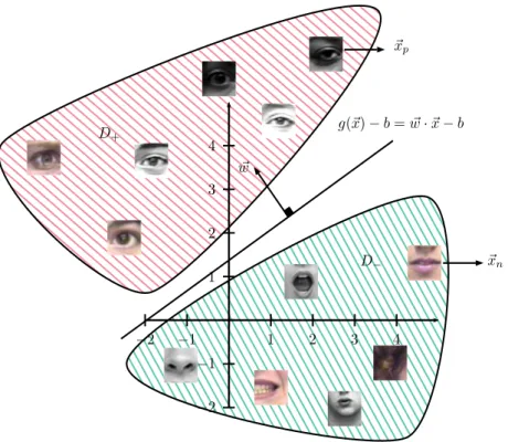
Definition 2.4.2 (Linearly separable set) A training set D is linearly separable if there is a linear function g:Rn→R such as
g(~x)−b >0, if(x, y)∈D+, g(~x)−b <0, if(x, y)∈D−.
(2.10)
where b∈R.
1 2 3 4 −1 −2
1 2 3 4
−1
−2
~ w
g(~x)−b=w~·~x−b
~xn
~xp
D+
D−
Figure 2.9: Linearly separable training set where ~xn and ~xp are false positive and true positive sample respectively resulting of the Viola and Jones detector. A linear functiong(~x)−b=w~·~x−b= 0 classifies these samples eye regions insideD+ and D−.
It is not difficult to notice that linear function gˆ, in perceptron model, is a good alternative for function g−b (with w0 = −b) but the problem is how to construct function g and find a
suitable b to solve a binary classification problem in an optimal way. A better approach to find both g and b was present in 1992 by Vladimir Vapnik and his team of AT&T Labs in [Vapnik, Boser and Guyon 1992] called Support Vector Machine or simply SVM. Based in the empirical risk minimization (ERM) [Vapnik 1992] and formalized in probability theory [Vapnik and Chervonenkis 1971], Vapnik concluded that the problem of finding a linear function g(~x) =w~ ·~xand b to solve the binary classification problem taking a linearly separable training set D can be solved through the solution of a convex optimization problem (DP) [Hamel 2009] of the form
(DP)
arg min ~ α
h(α~) = arg max
~ α ( l X i=1
αi−1
2 l X i=1 l X j=1
αiαjyiyjxi~ ·xj~ )
subject to l
X
i=1
αiyi = 0,
αi ≥0 for i= 1, ..., l.
(2.11)
where l is the cardinality of the set E,w~∗ =Pl
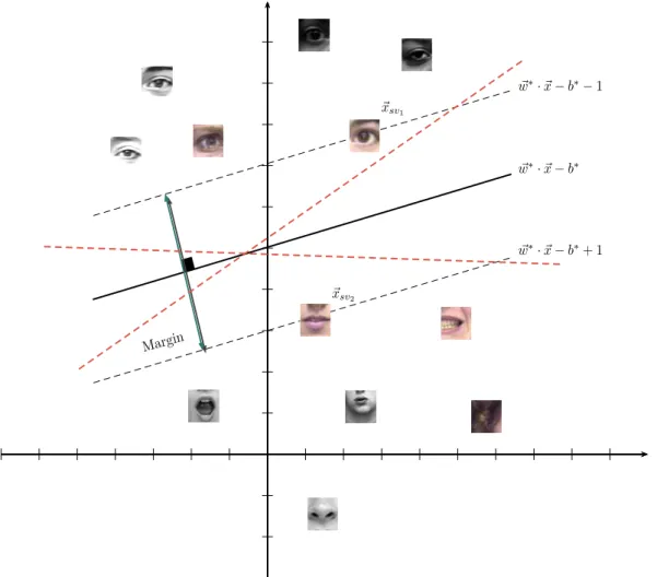
find the optimum values w∗ and b∗ for g(~x)−b can be understood like finding a linear function
that separates the sets D+ and D− better. This separation is associated with a concept called
maximum margin associated in turn with two parallel functions as shown Figure 2.10. This means that the greater the margin or the greater the distance separating the functions g(~x)−b+ 1 = 0
and g(~x)−b−1 = 0, classification is better. Finally, optimal linear function w~∗·~x−b∗ = 0 can
Margin
~xsv1
~xsv2
~
w∗·~x−b∗−1
~
w∗·~x−b∗+ 1
~ w∗·~x−b∗
Figure 2.10: A geometric sample of SVM approach. Solving problem(DP)and based in an support vector, in this case ~xsv1 or ~xsv2, the optimum values w~
∗ and b∗ for g(~x)−b = w~ ·~x−b = 0 are
calculated. The red dotted lines are not optimal linear functions.
be used to classify an element~xs∈/E with a decision function (likefˆin Perceptron model) of the form
f(~xs) =
y+, if w~∗·~xs−b∗>0,
y−, if w~∗·~xs−b∗<0,
(2.12)
wherey+, y−∈Y and~xs∈Rn. With decision functionf is possible solve the binary classification problem based in a linear separable set Dbetter than in Perceptron model. However, there still is a challenge related with D to solve in a real-life problems.
or decision problem related with a training set D linearly separable. For this reason the SVM version presented above can not be used for most real world problems such as eye detection. However, there is a way to deal with non-linearly separable training set using an approach called Kernel Trick.
In 1964 information theorist Thomas M. Cover in his research about pattern recognition [Cover 1965] proposed one way to map the elements in a non-linearly separable set DwhereE is in some input space (usually in Euclidean spaceRn) to an spaceHwith high dimension, possibly infinite,
where the mapped element are possibly linearly separable. Formally, His an Hilbert space called feature space but the notion about this concept will be more important later. To understand well the linearly separability of a training set D in this new space it is necessary define the concept of φ-separable.
Definition 2.4.3 (φ-separable) Let E ⊂ Rm0 and H is an m
1-dimensional space. A mapped
training set D¯ ⊂ H isφ-separable if there is an m1-dimensional vector w~ ∈ H such that
~
w·φ(x)−b >0, if (φ(x), y)∈D¯+, ~
w·φ(x)−b <0, if (φ(x), y)∈D¯−,
(2.13)
where D¯ ={(φ(~x), y) :~x∈E∧y∈Y},φ:E⊂Rm0 →His a map that take the elements of E to
H when m1 > m0.
Here, D¯+ = {(φ(x), y) : y = y+} and D¯− = {(φ(x), y) : y = y−} satisfy D¯ = ¯D+∪D¯− and ¯
D+∩D¯− =∅according to Definition 2.4.2.
Notice that if D¯ is linearly separable in H it is possible to use SVM approach to classify its elements in that space. But, how to guarantee that bringing the elements of E ∈Rm0 to
H, its mapped elements will be linearly separable. The response to this question is in Cover theorem.
Theorem 2.4.1 (Cover theorem) If P r(N, m1) is the probability of separation in D randomly
selected be φ-separable, then
P r(N, m1) = (
1 2)
N−1
m1−1 X
k=0
N−1
k
, (2.14)
where N is the cardinality ofE ⊂Rm0 and m
1 is the dimension ofH.
According to Theorem 2.4.1 is possible guarantee that when the dimension of H increases, the probability of linear separability of D¯ based on E and some suitable φ, increases too. So, it can
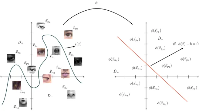
use SVM approach in D¯ to solve the binary classifier problem in E ⊂Rm0 as shown Figure 2.11. Now, the non-linearly separability problem of DwithE ⊂Rm0 andY =
{y+, y−}was reduced to
construct a suitable map φ such that D¯ is linearly separable and how to operate problem (DP)
D+
D−
φ
~xp1
~xp2
~xp3
~xn3
~xp4
~xp5
~xp6
~xn1
~xn2
~xn4
~xn5
~xn6
φ(~xp1)
φ(~xp2)
φ(~xp3)
φ(~xp5)
φ(~xp4)
φ(~xp6)
φ(~xn1)
φ(~xn3)
φ(~xn2)
φ(~xn5)
φ(~xn4)
φ(~xn6)
s(~x) w~·φ(~x)−b= 0
ˆ D+
ˆ D−
Figure 2.11: Non-linearly separability of D=D+∪D−whereD+={(~xp1, y+),· · · ,(~xp6, y+)}and
D−={(~xn1, y−),· · ·,(~xn6, y−)} is translated to a linearly separability ofD¯ = ¯D+∪D¯− based on
E ={~xp1,· · ·, ~xp6, ~xn1,· · ·, ~xn6}. Left graph represent the input space and right graph represent
H space whereD¯ is linearly separable based onDand φ.
can build a map Φ of the eigenfunctions decomposition of a definite positive function k called kernel or Mercer function. That is, if kis the continuous kernel of a integral operator K,
K:L2 →L2 f → Kf
(Kf)(y) =
Z
k(x, y)f(x)dx, (2.15)
which is defined positive, i.e,
Z
f(x)k(x, y)f(y)dxdy >0 s.t. f 6= 0, (2.16)
then kcan be expressed as a series
k(x, y) =
∞
X
i=1
αiψi(x)ψj(y), (2.17)
with positive coefficients αi, and
(ψ(x)·ψ(y))L2 =δij, (2.18)
for i,j∈N. By (2.17), can be extracted
Φ(x) =
∞
X
i=1 √
(2.19) is the map that leads the input data in Eto a Hilbert space Hwith higher dimension where k has the properties of an inner product, i.e,
k(x, y) = Φ(x)·Φ(y). (2.20)
By (2.20) and the fact that Hilbert spaces preserve the geometric properties of Euclidean spaces it is possible to use the continuous kernel kto measure the similarity between the elements inside the Hilbert space H operating in the input space without knowing Φ. The existence of H was demonstrated in the work of Nachman Aronszajn [Aronszajn 1950] and Vladimir Vapnik [Vapnik and Cortes 1995].
So, replacing~xi·~xj withφ(~xi)·φ(~xj) in(DP) can be used the inner product properties (2.20) to solve the convex optimization problem inHwhereD¯ is linearly separable operating inE⊂Rm0 (input space). There are many kernels known in the state-of-the-art to do that, as shown Table 2.1, and each of them can solve a problem well than other but in classification problems it is preferred to use Gaussian kernel because it usually represent better non-linearly data in the feature space according to the results obtained in [Bo, Ren and Fox 2010, Bo and Sminchisescu 2009].
Kernel Trick can be used in other approaches related with supervised learning or unsupervised learning too. On the other hand, kernel theory is used in different way for object recognition to construct a novel type of descriptor that can used to extract different features. It details more than this in the next section.
Kernels known
Kernel name Kernel Parameters
Linear kernel K(~x, ~y) =~x·~y none Homogeneous polinomial kernel K(~x, ~y) = (~x·~y)d d≥2 Nonhomogeneous polinomial kernel K(~x, ~y) = (~x·~y+c)d d≥2, c >0 Gaussian kernel K(~x, ~y) =e−λ||~x−~y||2
whereλ= 21θ2 withθ >0
Table 2.1: Most common kernels used in the state-of-the-art in different learning tasks and machine learning approach. Hereλis called radial parameter andθ2 is related with the variance in a normal
distribution.
2.4.2 Learning with kernel methods in object recognition
255 255 255 215 85 125 85 197 36 154 55 35 21 17 39 127 79 163 201 43 198 223 225 220 97
Figure 2.12: Eye information is not inside all the image only in a part of it. This is shown taking gray-scale image of CK+ database as a sample. The matrix values in right bottom are not the real values.
One of the most popular approaches to deal with this problem is Bag of Words methods or simply BOW. This method characterize an image as a local feature set. Formally, let X =
{x1,· · · , xp} a set of local features (e.g. HOG features details in Section 2.3) of a image and
V ={v1,· · ·, vn}1 a set of features defining some object of interest, sometimes called dictionary. In BOW, each local feature is quantized in a n-dimensional binary feature vector
µ(x) = [µ1(x),· · · , µn(x)], (2.21)
where µi(x) is 1 ifx ∈R(vi) and 0 otherwise. Here R(vi) = {x:||x−vi|| ≤ ||x−v||,∀v∈V}is the area where x is similar to vi using a suitable metric. The local features vectors for an image formed a normalized histogram µ¯(X) = |X1|P
x∈Xµ(x), where | · |is a cardinality of a set. Notice thatµ¯(·)can be used to measure the similarity between two different images through of its features sets. That is, let X and Y feature sets of two different images, it is defined
KBOW(X, Y) = ¯µ(X)Tµ¯(Y)
= 1
|X||Y|
X
x∈X
X
y∈Y
µ(x)Tµ(y)
= 1
|X||Y| X
x∈X
X
y∈Y
f(x, y),
(2.22)
as a measure of similarity. It is easy to show [Bo and Sminchisescu 2009] that f(x, y) is a Mercer kernel and due to the closure property of the kernels, KBOW is a Mercer kernel too. This approach
allows measure the similarity of two images or patch of images with suitable local features selected (e.g. HOG or SIFT features) without use a type of machine learning approach.
Calculate the kernel KBOW required a computational cost of O(|X||Y|)and when this is used with a kernel machine (e.g. SVM) has O(N2) and O(N2n2d) for storage and calculate the total
kernel matrix, respectively, where N is the number of images in the training set, and m is the average of cardinality of all sets. For image classification, m can be in thousands of units, so the computational cost quickly becomes of four grade when N tends to m (or tend to infinity). This make thatKBOW can not use for real-time detection systems in surveillance context because its high computational cost to calculate it. To address this, it can take a kernel k(x, y) instead of f(x, y) in (2.22) and not calculate it directly if not built a map Φ based in its inner product properties shown in (2.20) such that
Ks(X, Y) =
¯
Φ(X),Φ(¯ Y)
, (2.23)
where Φ(¯ X) = 1
|X|
P
x∈XΦ. If Φ(¯ X) is finite, it is possible to explicitly calculate and use it for mapping features and obtain finite descriptors that can be train trough a linear classifier (e.g. SVM). The train and test cost of this learning process is O(N mDd) and O(mDd), respectively, where dis the dimension of the elements in some X andD is the dimension of mapping Φ(x). If the dimension of Φ(x) is low, the computational cost of this approach can be much lower than required through the calculate of the kernel functions. For example, the cost can be 1
N much lower when D belongs the same order than m. Note that for this method is not necessary to calculate the total kernel matrix but just the mapping Φ(¯ X). This type of feature descriptor is called kernel descriptor and there is only one problem to apply this approach related with the explicit construction of Φ(¯ X).
In practice is not easy to built a mapΦrelated with some kernelk(x, y)because often it has a high dimension (possibly of infinite dimensional) and not all the maps lead to a significant similarity measure for determiner recognition problems. For this reason, in [Bo and Sminchisescu 2009] was proposed an approach to calculate an approximation of Φ with which is possible approximate features maps based in a set of basis vectors related with the object of interest. This approach is called Efficient Match Kernel (EMK) and we will explain more about it.
LetH a Hilbert space having as elements all the features vectors of the form ψhigh(x), where
high refer that the dimension of the space is very high. Due of this difficult, the idea for approximate features maps is project ψhigh(x) to an features vector ψ(x) within of an sub-space of H of low dimension based on a set of d1 feature vectors, so build a local kernel through the inner product
of the approximations. Formally, let {ψ(zi)}di=11 , a set of mapped basis vectors zi. Then, it can approximate a feature vector ψ(x)of the form
¯
vx= arg min vx
||ψ(x)−Hvx||2, (2.24)
The program (2.24) is really a convex optimization problem with unique solution
¯
vx = (HTH)−1(HTψ(x)), (2.25) so the local kernel derived of the project vectors is
klow(x, y) =hHv¯x, Hv¯yi=kZ(x)TKZZ−1kZ(y), (2.26) where kZ is a vector d1 ×1 with {kZ}i = k(x, zi) and KZZ is a d1×d1 matrix with {KZZij = k(zi, zj)}. ForGTG=KZZ−1 (whereKZZ−1 is positive define), the local features map is
Φ(x) =GkZ(x), (2.27)
and the total resulting feature map is
¯
Φ(X) = 1
|X|G "
X
x∈X
kZ(x)
#
, (2.28)
with a computational cost O(md1d+d21) for a set of local features. The constructing map can
be used with a linear SVM without kernel trick which allows optimize the computational cost of classification process.
In Chapter 3 is details the proposed approach to extract and train features that complement the results obtained by Viola and Jones detector. This approach is based in EMK and the linear version of SVM explained in this chapter.
2.5
Summary
In this chapter a brief review of the main works addressing the eye detection problem in multiple contexts and considerations that must be taken into account for real-time applications has been done. Especially, it is explained the approaches dealing better the challenges can be found in video surveillance context in uncontrolled environments.
First, we made a description of the work developed by Viola and Jones [Viola and Jones 2004] emphasizing its main contributions and disadvantages. Then, it was mentioned some current works based on Viola and Jones investigation to obtain better results in eye detection applications or systems. Due to of the low precision of the VJD in uncontrolled environments it made a brief review of the most important works that address the detection problem with more sophisticated methods where works as HOG [Dalal and Triggs 2005] and BOW [Felzenszwalb et al. 2010] are highlighted. Finally, it made an introduction of kernel theory to envelop the reader with the basis enough to understand research related with SVM [Vapnik and Cortes 1995] and EMK [Bo and Sminchisescu 2009].
Chapter 3
The proposed methodology
3.1
Introduction
In this chapter is described the methodology used to develop the eye detector proposed in this work. Section 3.2 exposes a sample problem to be solved using two types of database. Section 3.3 present details about features used in Viola and Jones work and why is important to complement it with other types of features. Section 3.4 describe all the methods that will be used to solve the problem of eye detection in unconstrained context. Finally, Section 3.5 details the proposed approach design using the resulting outputs of Viola and Jones detector as input data.
3.2
Eye detection problem in unconstrained settings
Many works about eye detection [Awais, Badruddin and Drieberg 2013, Chen et al. 2014, Choi, Han and Kim 2011, Hyunjun, Jinsu and Jaihie 2014, Oliveira et al. 2012] inside the object recognition context in Computer Vision have been doing currently. However, it is not common that these type of research deals the problem in a unconstrained settings. In this work is addressing the eye detection problem in unconstrained environments but without ignoring features such as performance and accuracy of detection. For do this, it is necessary introduce the reader inside both constrained and unconstrained contexts.
(a) Neutral expression. (b) With expression.
Figure 3.1: A samples of CK+ database [Lucey et al. 2010].
For detection problems in real life, for example in surveillance context, the collected images for detection usually are in unconstrained environments. FDDB database [Jain and Learned-Miller 2010] is not a database that contain images of surveillance environments but has an image collection of people captured in unconstrained environments. As shown Figure 3.2, it is not possible to know what type of environment we will have in a situation in real life and what type of detection challenge it will present. There are many challenges in this type of context that hindering detection task such as occlusion, non rigid variation, deformation, photometric, viewpoint and variable structure. To address these challenges in eye detection it is propose an approach based in EMK explained in 2.4.2 that can extract a complementary local features of the VJD resulting outputs in a fast way.
3.3
Viola and Jones detector as a first layer
The research made by Viola and Jones [Viola and Jones 2004] is one of the most popular in the object detection area. Currently, it is used in detection of several objects as humans, faces, eyes, cars or pets and it is used as support of many research in the state-of-the-art too. This is because the capacity of Haar-like features (explained in Chapter 2) to extract information patterns in the input image helping in final detection of the object of interest. In addition, the calculating necessary for each detection is not expensive than in other approaches because the integral image representation and the form to calculate it. However, the Viola and Jones detector has a disadvantage related with its results obtained in real life contexts. Due to the unconstrained environments several amount of false positives are obtained and this rules out its use in surveillance detection systems. A sample this is shown in Figure 3.3.
(a) Carmen Electra in a unconstrained lighting environment.
(b) George Bush in real life situation with a complex background
(c) A man with complex background. (d) A tennis player in action.
(a) BIOid. (b) CK+. (c) FERET. (d) FDDB.
Figure 3.3: Samples of resulting outputs of Viola and Jones detector.
Figure 3.4: Flow diagram of cascade classifier with efficient kernel detector. Here, Viola and Jones detector is used to generate outputs and then an efficient kernel approach based on HOG features and a linear classifier are used to improve the results.
is used to discriminate the false positives of the true positives. It will be demonstrated that with this approach is possible to discard up to 98% of false positives of the Viola and Jones detector.
3.4
EMK and SVM for eye detection
The simplicity of Haar-like features used in the Viola and Jones detector (VJD) [Viola and Jones 2004] introduce a high amount of false positives in the resulting outputs in uncontrolled environments. This can be related to the object of interest and how is projected inside the image. In the case of the eye detection in a unconstrained environments, many of the patterns that represent to the eye through of the Haar-like features can be confused with the features found for other objects (or simply part of the background) in the image environment. In addition, it is not easy deals with eye recognition in unrestrained environments even for the human eye. For example, looking in Figure 3.3.d a mouth can be mistaken for an eye if you take a quick look. To addressing this problem in an eye detector it is possible use a second type of features that are capable to extract patterns with which possible difference between a false positive of a true positive region and address the usual challenges presented in this type of detection.
Figure 3.5: Green square in a output represent the structure of one HOG feature composed by 4 cell with 9 bins for each one. Based on the work of Dalal and Triggs [Dalal and Triggs 2005], it is enough consider the 9 oriented bins in 0◦−180◦. According to that, it will has 36 dimensions per features.
train a SVM classifier. That is, let E ={X1,· · · , XL} a set of VJD resulting outputs. Suppose that each output has tp×tp pixels and a block structure per output as shown in Figure 3.5. Then the amount of features c per output is defined as
c=
tp
S +p× tp
S
×
tp
S +p× tp
S
, (3.1)
where S ×S represent the dimension per block and p is the step size between features. If we consider bbins and 4 cells per block, the HOG features representation for an output is defined as
Xs = (xs1,· · ·, xsc) ∈ Rb×4×c with s = 1,· · ·, L. Here xsm with m = 1,· · · , c represent a local features of the output Xs. So, it is possible to solve the optimization convex problem(DP) (2.11) based on E using this feature structure constructing a decision function like (2.12) of the form
f(Xs) =
+1, if w~∗·X
s−b∗ >0,
−1, if w~∗·Xs−b∗ <0,
(3.2)
whereXs∈/ Eis an unlabelled output to classify,+1 :represent an eye detected and−1 :represent an not eye detected. This approach is a good way improve the results of the detection. However, it is not guarantee that the training set D(based onE) is linearly separable. Although that could be solved using Kernel Trick, there is a better solution using Efficient Match Kernel (EMK).
(a) HOG features in false positives.
(b) HOG features in true positives.
Figure 3.6: HOG features samples extracted of the Viola and Jones resulting outputs using FDDB database. It is possible to see the difference between the false and true positives looking inside their HOG features.
on E through a special map related with the Mercer conditions 2.16. The key of this approach is based on EMK which need a set of mapped features vectors {ψ(zi)}d1
i=1, withzi ∈Z, to construct
a approximation of map Φ¯ as shown equation (2.27). In the case of eye detection,Z represent the basis vector set based on HOG local features that represent better one eye. To understand this, suppose that setZ is defined through three elements of a sampleX1= (x11, x12, x13, x14)such that Z ={x11, x12, x13}. This means that all the mapped elements of Z withΦ forms a generator set
of the space HZ where local features of any other mapped sample Xs = (xs1, xs2, xs3, xs4), with
the sameΦ, can be represented as weighted sum of the elements ofZ as shown Figure 3.7. Also, it could be calculated the similarity of local mapped features of two different samples inHZ through a suitable metric, norm or even a kernel defined inside this space.
Using this approach can be used the mapΦ¯ to construct descriptors based on the samples ofE
generating a descriptors set of the form{Φ(¯ X1),· · ·,Φ(¯ XL)} in a high dimension space where the training set D¯ could be linearly separable. So, it is possible to train a learning machine like SVM
to construct a linear classifier to identify if a sample Xs ∈/ E is an eye or not. This method only introduce an additional step when the elements of Z are found through a unsupervised learning method as PCA [Barber 2012] or K-Means [James et al. 2013]. However, this does not affect the last detection performance.
3.5
Efficient kernel eye detector design
X1= (x11, x12, x13, x14) x11 x12 x13
Φ
Φ(x13)
Φ(x12)
Φ(x11)
HZ
Z=
b
Φ(xs1) =c1Φ(x11) +c2Φ(x12) +c3Φ(x13)
Figure 3.7: HZ is constructed based on a setZ ={x11, x12, x13}of HOG local features generated
using the outputs of VJD and mapΦ. LetXs= (xs1, xs2, xs3, xs4), a mapped local feature can be
represented as Φ(xs1) in this space based on{Φ(x11),Φ(x12),Φ(x13)} wherec1, c2, c3∈R.
To simplify the implementation of the proposed method was used the version of the VJD in OpenCV Library [Bradski 2000]. This implementation consider multi-scale detection but for our propose method we only use a standard size per output as input data because the ROIs were considerably reduced for VJD. This size depends on the structure chosen for the HOG feature extraction (in each stage) and the average dimension of the outputs labeled as true positive in each database. As shown Figure 3.5 and based on the work done by Dalal and Triggs in [Dalal and Triggs 2005], we going to consider atp×tpoutput and aS×S block composed of 4 cells with 9 bins per output for the construction of each descriptor HOG where tp ∈ {36,44,60,72}. This selection is related with the average dimension of the outputs labeled as true positive per database and motivated for one of features found in [Oliveira et al. 2012]. It will be seen in Chapter 4 that this structure will take a good experimental results.
On extraction stage a HOG features framework is adopted to characterize each ROI. Then, K-Means [James et al. 2013] clustering is used to find a basis vector set Z, as shown Figure 3.8 where z1, z2,· · · , zKc are the centroids founded with the method. The idea is to extract the more important features defining one eye and differentiate them from other objects (e.g, part of the environment or part of other objects) on a subregion of the ROI. It forms a feature eye space where the similarity between parts of different ROIs can be measured. The algorithm that implement this stage is shown in Algorithm 1.
. . .
x11 x12 . . . x1l x21 x22 . . . x2l x31 x32 . . . x3l xL1 xL2 . . . xLl
z1
z2
zKc
. . .
Z = [z1, z2, z3,· · ·, zKc]
Figure 3.8: Extraction stage - In extraction stage the basis of features vectors is found and then these are used to construct the kernel descriptors in training stage. X1 = {x11, . . . , x1l}, X2 = {x21, . . . , x2l}, . . ., XL ={xL1, . . . , xLl}are the L features sets of L true positives outputs of the VJD that will be the input data for an unsupervised learning method to find a basis set Z with
Data:
{X1, X2· · · , XT}: A set of resulting ROIs of Viola and Jones detector;
tp: Size of a ROI side;
S: Size of a block;
Result:
G: A matrix to construct Efficient Kernel Descriptors as shown in (2.27);
Z: A matrix containing all the basis vectors;
Kc: Clusters number;
Parameters: Initialization
K: A matrix in (2.26);
c: Amount of features per ROI defined as tp S +p×
tp S
× tpS +p× tp S
; descriptorValues: Array containing the HOG features extracted per ROI;
P s: A matrix that containing the information of the HOG features of all ROIs where
P s(i,·) is a feature vector;
p= 0.5: size step per features;
j= 1;
fori= 1 ; i≤T do
ToGrayScale(Xi); Equalize(Xi); Resize(Xi,tp);
descriptorValues[i] = HOGDescriptor(Xi);
fork= 1 ; k≤cdo
P s(j, k) = descriptorValues[i];
j+ +;
end end
Z = FindCentersKmeans(P s,Kc);
K = ConstructK(Z);
K−1 = InvertMatrix(K);
G= CholeskyDescomposition(K−1);
return (Z,G)
Data:
{X1, X2· · · , XTe}: A set of resulting ROIs of Viola and Jones detector; tp: Size of a ROI side;
S: Size of a block;
G: A matrix to construct Efficient Kernel Descriptors as shown in (2.27);
Z: A matrix containing all the basis vectors;
Result:
f: Decision function from SVM model;
Parameters: Initialization
c: Amount of features per ROI defined as tp S +p×
tp S
× tpS +p× tp S
;
p= 0.5: size step per features;
descriptorValues: Array containing the features extracted per ROI;
F v: A matrix that containing the information of the features of each ROIs;
Kd: Kernel descriptor;
fori= 1 ; i≤Te do ToGrayScale(Xi); Equalize(Xi); Resize(Xi,tp);
descriptorValues[i] = HOGDescriptor(Xi);
fork= 1 ; k≤cdo
F v(k)= descriptorValues[i];
end
Kd = ConstructEfficientKernelDescriptor(F v,Z,G); trainData(i) = Kd;
if Xi is True positive then labelData(i) = 1;
else
labelData(i) = 0;
end end
f =ConstructDesicionFunctionSVM(trainData,labelData); return (f)
X1 X2 X3 XN
. . .
x11 x12 . . . x1l x21 x22 . . . x2l x31 x32 . . . x3l xN1 xN2 . . . xN l
¯
φ(X1) =|X1 1|G
h P
x∈X1kZ(x)
i
¯
φ(X2) =|X1 2|G
h P
x∈X2kZ(x)
i
¯
φ(X3) =|X1 3|G
h P
x∈X3kZ(x)
i
¯
φ(XN) =|X1 N|G
h P
x∈XNkZ(x)
i
. . .
SVM Training
f( ¯φ(Xt))
Figure 3.9: Training stage - In training stage the kernel descriptors are trained in a linear Support Vector Machine. For this, it is necessary supervised input data, that is, we need to label kernel descriptors generated with the output of the VJD. Here,X1, . . . , XN are the sets of features which would be used to construct the kernel descriptorsφ¯(X1), . . . ,φ¯(XN). These descriptors are labelled as eye or other thing for the training. As a result, after training, a decision functionf(·)is obtained that will be used to the eye detection.
descriptor which is labelled as eye or non-eye. Finally, these labelled descriptors are used to train a linear SVM to obtain a linear classifier f(·)as shown Figure 3.9. This classifier is constructed in a feature space where the mapped input data is probably linearly separable. The algorithm that implement this stage in shown in Algorithm 2.
Finally, on classification stage, an efficient kernel descriptor is constructed based on an unla-belled output and it is launla-belled by the linear classifierf(·)built on training stage. This classification is essentially the final detection task of the proposed method. This is show in Figure 3.10 and the reader can see the algorithm that implement this stage in Algorithm 3.
3.6
Conclusion
In this Chapter it was present a proposed methodology of an eye detector based on an Efficient Match Kernel approach and we will try to improve the precision of the well-know VJD using it. The idea is used this propose to complement security and surveillance systems where it is require a fast response and high precision to alert users.
Proposed eye detector takes ROIs resulting of Viola and Jones detector and extract local features based in kernel theory. This features can be used as a complement for Haar-like features used in the work of Viola and Jones without increase significantly its computational cost and improve its precision though of a linear SVM. It used a cascade architecture and a linear classifier to discriminate false positives such that the precision is improved in the final detection.
![Figure 2.7: A sample of scene recognition made in [Pandey and Lazebnik 2011]. Left column: root and part filters based HOG features](https://thumb-eu.123doks.com/thumbv2/123dok_br/16853837.753295/26.892.119.782.572.793/figure-sample-recognition-pandey-lazebnik-column-filters-features.webp)