January 3rd, 2020
Forecasting Banking Crises in Developing Countries: a Dynamic
Probit Approach
Diogo Carvalho Costa – 33785
A project carried out on the Master’s in Finance Program under the supervision of:
- 1 -
Abstract
Banking crises have afflicted economies in developing countries at least as much as they have in developed ones. In this paper, we discuss possible indicators that allow an effective forecast of banking crises based on an historical analysis of past crises, and develop several probit models, using yearly data from 1960 to 2014 for 33 developing countries across Latin America, Africa and Asia-Pacific. We find that a dynamic probit model which incorporates exuberance dummy variables gives the best forecasting results. Data on exports, inflation, broad money and birth rate provide the best indicators across the different models tested.
- 2 -
1. Introduction
Banking crises have sprouted around the world throughout the past century, having reached their climax on the turn of the past decade. They have given rise to major setbacks on general economic welfare, affecting developed and developing countries alike. These events often stem from the risk exposure inherent to banking institutions which finance long-term investments with short-term deposits, leaving them vulnerable to the so called “bank runs”: situations in which large portions of the depositors demand their deposits back, forcing banks to liquidate long-term investments at sub-optimal prices (Goldstein & Razin, 2013).
In this paper, we adapt the approach developed by Antunes, Bonfim, Monteiro, & Rodrigues (2018) to develop an early warning system for banking crises in developing countries using yearly data from 1960 to 2014. Three models are tested: a Simple Probit Model, a Dynamic Probit Model, and a Dynamic Exuberance Probit Model. The indicators used in the forecasting models were chosen after extensive reading of literature focused on previous banking crises, with particular emphasis on Latin American countries where these events were most recurrent, along with variables used in similar, previously developed Early Warning Systems. The final models include Total Debt Service (%Exports), Total Reserves (%Total External Debt), Birth Rate, Broad Money Growth, Current Account (%GDP), Domestic Credit provided by the Financial Sector (%GDP), Domestic Credit to Private Sector (%GDP), Exports of Goods and Services (%GDP), External Balance on Goods and Services (%GDP), GDP Growth, and annual Inflation of Consumer Prices, as well as dummy variables for past crisis events and exuberance in the variables.
The aim of this paper is to shed more light on the causes behind banking crises in developing countries and provide the best indicators to forecast such events, while corroborating the validity of dynamic probit models as forecasting tools by applying the methodology of Antunes, Bonfim, Monteiro, & Rodrigues (2018) on a completely different dataset. Another contribution comes from
- 3 -
further investigating the potential use of demographical variables as indicators for financial distress, rooted on the assumption that shifts in the financial well-being may have an influence on family planning, and thus be reflected in variables such as Birth Rate.
The paper is organized as follows: in Section 2 we explore the core of the literature review, highlighting the major causes of past baking crises; Section 3 comprises the explanation of the data used in the models; in Section 4 we discuss the methodology applied; Section 5 offers an analysis of the results from the several regressions; and Section 6 summarizes our main conclusions and findings, while exploring our limitations and suggesting further research.
2. Indicators from the past
Financial collapses have haunted developing countries in the past, with resolution costs (sometimes reaching as high as $250 billion) hindering the development of government programs for fiscal consolidation (Honohan, 1997). It would be unreasonable to aim at identifying and preventing every single bank failure, but to avert the occurrence of systemic banking problems should be one of the main goals among policy makers. In order to do so, one must take a closer look into some of the main banking crises of the past and understand the underlying factors which are common across them. The three main regions of analysis in this paper are Latin America, Africa and Asia-Pacific, with the first naturally taking the limelight as there is evidence that, between 1970 and 1995, it suffered 50 percent more crises per country than East Asian, European or Middle Eastern countries (Kaminsky & Reinhart, 1998).
Endogenous macroeconomic instability has often been at the core of banking crises in Latin America. Boom and bust cycles have been common in the past, with banks over-investing in optimistic times, giving rise to the number of defaults with ruinous consequences in the following
- 4 -
years, the bust phase of the cycle. This was the case for Argentina, Chile and Uruguay in 1979-83, as well as Mexico in 1994 (Honohan, 1997).
In the years that led to the crisis in the early 1980s, Argentina faced high rates of inflation and serious balance of payments’ problems, as well as a considerable fiscal deficit. Growing lending rates and financing of high-yield but high-risk projects, as well as rocketing nominal interest rates and a lack of adequate supervision, were at the heart of the crisis (Baliño, 1987). The 1990s banking crisis in Argentina was accompanied by a currency crisis and it was marked by current account deficits, low level of domestic savings, and a worsening fiscal position (García-Herrero, 1997).
As for Chile, the period between 1974-81 was marked by economic reforms which initiated the boom phase of the business cycle. New and raising expectations about the country’s potential allowed for an increase in domestic private demand, fostered by renewed access to domestic and foreign loanable funds, operated by private national banks. Eventually, excessive risk taking by banks and changes in relative prices opened way for a banking crisis (Barandiarán, & Hernández, 1999). Financial liberalization in the absence of a proper regulatory framework is also pointed as a factor in the Chilean crisis of 1984 (Carstens, Hardy, & Pazarbasioglu, 2004; Kunt, & Detragiache, 1998). Kunt & Detragiache (1998) highlight foreign currency loans as a source of banking problems for Chile at this time, while Honohan (1997) stresses poor management and the assumption of risky open foreign exchange positions as important factors.
The Mexican Peso crisis of 1994 was linked to “disaster myopia”, a phenomenon that occurs whenever managers neglect negative events deemed unlikely (Honohan, 1997). The crisis was boosted by drastic changes in the banking system due to swift liberalization (Honohan, 1997; Griffith-Jones, 1998) which happened, as was the case of Chile, without appropriate regulatory
- 5 -
measures (Carstens, Hardy, & Pazarbasioglu, 2004). Large current account deficits are also pointed out as a main factor on the brink of the crisis (Griffith-Jones, 1998).
Often associated with poor management and lack of supervision, fraud can also be at the heart of banking crisis. This was the case in Venezuela in 1994 (Honohan, 1997). Other factors such as terms of trade shocks or abnormal movements in real exchange rates (Carstens, Hardy, & Pazarbasioglu, 2004), as well as the presence of an unstable or unreliable political environment (García-Herrero, 1997; Honohan, 1997), have also led the country into banking hazard.
Turning our attention to Africa, we can also find traces of mislead political decisions associated with fraud which have caused large insolvencies in state owned banks in Nigeria, in 1993 (Honohan, 1997). Sanusi (2010) also points to macroeconomic instability associated with large capital inflows, and overall lack of transparency and regulatory measures as causes for the banking failures across Nigeria in the past. In Ghana, non-performing loans have stirred banking volatility, led by variations in macroeconomic variables such as inflation, real GDP per capita growth and real effective exchange rates (Amuakwa–Mensah, & Boakye–Adjei, 2015).
Lastly, we can examine the conditions which originated and enflamed the financial crisis all across Asia-Pacific in 1997. Although some of these were initially currency crises,
“As the dust settles in currency markets, many of these countries will be left [and indeed were] with serious banking sector problems, if not full-scale banking crises”,
Kaminsky & Reinhart (1998).
There is evidence that the banking systems in this region were overall fragile even before the onset of the crisis (Corsetti, Pesenti, & Roubini, 1999), with the growing volume of short-term flows mostly intermediated by poorly regulated and otherwise ill-supervised domestic banking
- 6 -
sectors (Kaminsky & Reinhart, 1998). In the Philippines, outright fraud contributed to the fragilization of the banking system, with the loan losses of two large banks bailed out in the 1980s enriching the president and his associates, directly or indirectly (Honohan, 1997). Indeed, bailout costs are estimated to range from 7 percent of GDP in the Philippines to more than 20 percent of GDP in Thailand (Kaminsky & Reinhart, 1998).
Corsetti, Pesenti, & Roubini (1999) suggest that the data on the growth of bank credit to the private sector and the ratio of private sector lending to GDP point towards a lending boom in the 1990s across East Asian countries. They also find evidence of deteriorating quality of loans by observing a growing percentage of non-performing loans. This was again, as across countries in other regions, related to mishandled financial liberalization, excessive lending in highly risky projects and lack of commitment to regulatory actions in countries such as Thailand, Indonesia and Malaysia.
3. Data
The data selected for the development of this paper’s early warning system was chosen not only by analyzing past banking crises, as discussed in the previous section, but also by considering the variables used on similar warning systems in the past. All data was retrieved from the World Bank, except for the Crisis dummy variable.
The Crisis dummy variable was taken from the Harvard Business School’s Behavioral Finance & Financial Stability project database on Global Crises Data by Country, collected by Carmen Reinhart, Ken Rogoff, Christoph Trebesch and Vincent Reinhart. It includes a dummy variable for Banking Crisis for more than 70 countries and over 200 years. However, for this paper, the variable was considered from 1960 until 2014, for a set of 33 developing countries.
- 7 -
The countries selected can be divided geographically in three groups: Latin American countries (Argentina, Bolivia, Brazil, Chile, Colombia, Costa Rica, Dominican Republic, Ecuador, El Salvador, Guatemala, Honduras, Mexico, Nicaragua, Panama, Paraguay, Peru, Uruguay, and Venezuela); African countries (Cote d’Ivoire, Egypt, Ghana, Kenya, Morocco, Nigeria, South Africa, Zambia, and Zimbabwe); and Asia-Pacific countries (China, India, Indonesia, Malaysia, Philippines, and Thailand).
The variable Inflation of Consumer Prices was used to catch any movements related to macroeconomic mismanagement. It is measured by the consumer price index, reflecting the annual percent change in the cost to the average consumer of acquiring a given basket of goods and services.
Domestic Credit provided by the Financial Sector (%GDP) and Domestic Credit to Private Sector (%GDP) are meant to account for boom and bust cycles in credit concession, while serving as a proxy for financial liberalization.
To reflect the imbalances on the balance of payments and the overall international commercial position, the variables Current Account (%GDP), Exports of Goods and Services (%GDP) and External Balance on Goods and Services (%GDP) were used.
In order to account for adverse macroeconomic shocks which can destabilize the banking system, the variable GDP Growth (annual%) was retrieved.
The inclusion of the demographical variable Birth Rate, crude (per 1.000 people) was included to test whether variables seemingly out of the usual financial spectrum could aid predicting the occurrence of a banking crisis by reflecting behavioral changes on the populations’ behalf, following the rationale of Lopes, Machado, Huffstot, & Mata (2018).
Finally, we considered Total Debt Service (%Exports), Total Reserves (%Total External Debt) and Broad Money Growth (annual%) by building on the work previously developed by
- 8 -
Bussiere & Fratzscher (2006); Kaminsky, Lizondo, & Reinhart (1998); Antunes, Bonfim, Monteiro, & Rodrigues (2018); Drehmann & Juselius (2012); and Edison (2003).
4. Methodology
The bedrock for this paper’s empirical findings is set upon the application of binary response models. The theoretical foundations for the construction of the regressions closely follow the methodology applied in Antunes, Bonfim, Monteiro, & Rodrigues (2018). Likewise, the general model is composed by the dependent binary variable 𝑦𝑖𝑡, a banking crisis indicator for country 𝑖 in year 𝑡 which takes the value of one whenever a crisis occurs and zero otherwise; and a (1 × 𝑑) vector of exogenous variables 𝑋𝑖,𝑡−𝑘.
The 𝑦𝑖𝑡 variable follows a Bernoulli distribution, such that 𝑃[𝑦𝑖𝑡 = 1] = 𝑝𝑖𝑡 and 𝑃[𝑦𝑖𝑡 = 0] = 1 − 𝑝𝑖𝑡, while 𝑝𝑖𝑡 is dependent on an information set available at 𝑡 − 1, given by ℱ𝑡−1≔ 𝜎 { (𝑦𝑖𝑠, 𝑥𝑖𝑠), 𝑠 ≤ 𝑡 − 1 } . Following Kauppi & Saikkonen (2008) and Candelon et al. (2014), we model the conditional probability 𝑝𝑖𝑡 as a function of the variables in ℱ𝑡−1, and consider 𝑦𝑖𝑡 = 𝐼 (𝑦𝑖𝑡∗ ≥ 𝑢𝑖𝑡), where 𝐼(. ) is an indicator function, 𝑢𝑖𝑡 is an 𝑖. 𝑖. 𝑑. process and 𝑦𝑖𝑡∗ is a latent variable that is related to the conditional probability 𝑝𝑖𝑡 through the common cumulative distribution function of the random variables {𝑢𝑖𝑡}. Furthermore, 𝑦𝑖𝑡∗ = 𝐹−1(𝑝
𝑖𝑡), where 𝐹(. ) is a cumulative distribution function assumed to be monotonically increasing and twice continuously differentiable. Hence, the probability of a crisis event is given by the expected value of 𝑦𝑖𝑡 conditional on ℱ𝑡−1, i.e., 𝐸(𝑦𝑖𝑡|ℱ𝑡−1) = 𝑃(𝑦𝑖𝑡∗ ≥ 𝑢𝑖𝑡|ℱ𝑡−1) = 𝐹(𝑦𝑖𝑡∗) = 𝑝𝑖𝑡.
- 9 -
4.1 Model Specifications
To forecast banking crisis events, we consider three models. The first is a Simple Probit model depicted as 𝑦𝑖𝑡∗ = 𝛼 + ∑ 𝑥𝑖,𝑡−𝑘𝛽𝑘′ Ρ 𝑘 + 𝑢𝑖,𝑡 , (1)
where k, the number of lags used, is equal across the explanatory variables, and ranges from one to five years, Ρ ∈ (1, … , 5). When the full range of the lags is applied (Ρ = 5) we are looking at the Total Period model. We also considered two restricted models: one to assess the predictive power of the indicators closer to the crisis, which we called the Late Period model and in which k= {1, 2, 3}; and another to evaluate the effectiveness of the indicators when predicting a crisis earlier on, which we called the Early Period model and in which k= {3, 4, 5}. The distinction between Late Period and Early Period models will also be used in the next two models.
The second model analyzed is a Dynamic Probit model presented as
𝑦𝑖𝑡∗ = 𝛼 + ∑ 𝑥𝑖,𝑡−𝑘𝛽𝑘′ Ρ 𝑘 + ∑ 𝛾𝑘 𝑦𝑖,𝑡−𝑘 Ρ 𝑘 + 𝑢𝑖,𝑡 , (2)
where 𝑦𝑖,𝑡−𝑘 is the binary crisis indicator variable for country 𝑖 at time 𝑡 – 𝑘. The lags of 𝑦𝑖𝑡 are included based on the belief that the occurrence of a banking crisis in previous years may help forecast a similar event in the future. In other words, we now consider the possibility of time dependence in 𝑦𝑖𝑡 and try to capture its effect through a dynamic model.
Finally, the last model considered represents a Dynamic Exuberance Probit model,
𝑦𝑖𝑡∗ = 𝛼 + ∑ 𝑥𝑖,𝑡−𝑘𝛽𝑘′ Ρ 𝑘 + ∑ 𝛾𝑘 𝑦𝑖,𝑡−𝑘 Ρ 𝑘 + ∑ 𝐷𝑖,𝑡−𝑘𝑘 𝛿𝑘′ Ρ 𝑘 + 𝑢𝑖,𝑡 , (3)
- 10 -
where D𝑖,𝑡−𝑘𝑘 is a (1 × 𝑑) vector, such that 𝐷𝑖,𝑡−𝑘𝑘 ∶= (𝐷𝑖,𝑡−𝑘𝑘1 , 𝐷𝑖,𝑡−𝑘𝑘2 , … , 𝐷𝑖,𝑡−𝑘𝑘𝑑 ) and 𝛿𝑘’ (𝑘 = 1, … , Ρ) is a (1 × 𝑑) vector of parameters. 𝐷𝑖,𝑡−𝑘𝑘 is the dummy variable for exuberance, which takes a value of one whenever the value for the according variable in 𝑡 – 𝑘 is higher than its 0.75 percentile across the data available for country 𝑖. The latter variables are included in order to capture any additional effect that an exuberant behavior of explanatory variables may have on the forecast of a banking crisis.
The gradual differences implemented in the equations building from the first equation allow us to perceive the marginal benefit that these additions have on the predictive power of the initial model. In every equation constructed above, a forecast is easily achieved without the need for constructing an actual forecasting model for the explanatory variables. By using a set of explanatory variables available at 𝑡 – 𝑘 (with 𝑘 ≥ 1), a forecast for 𝑦𝑖𝑡 for every year is directly achieved.
4.2 Parameter Estimation
In non-linear models, such as the probit models described above, the parameters can be estimated using maximum likelihood. The probability distribution of the 𝑖th observation, when a random sample of 𝑛 outcomes of the binary variable 𝑦𝑖𝑡 is available and the probability of success is the same for all observations, is given by 𝑝𝑦𝑖(1 – 𝑝)1 – 𝑦𝑖. When the observations are mutually independent, the log-likelihood function is given by
𝑙𝑜𝑔 𝐿(𝑝𝑖𝑡) = ∑ ∑ 𝑦𝑖𝑡𝑙𝑜𝑔(𝑝𝑖𝑡) 𝑁 𝑖 = 1 𝑇 𝑡=1 + ∑ ∑(1 − 𝑦𝑖𝑡) 𝑙𝑜𝑔(1 − 𝑝𝑖𝑡) = 𝑁 𝑖 = 1 𝑇 𝑡=1 = ∑ ∑ 𝑦𝑖𝑡𝑙𝑜𝑔(𝐹(𝑦𝑖𝑡∗)) 𝑁 𝑖 = 1 𝑇 𝑡=1 + ∑ ∑ (1 − 𝑦𝑖𝑡) 𝑙𝑜𝑔(1 − 𝐹(𝑦𝑖𝑡∗)) , 𝑁 𝑖 = 1 𝑇 𝑡=1 (4)
- 11 -
since, as defined above, 𝐹(𝑦𝑖𝑡∗) = 𝑝𝑖𝑡. Maximizing the log-likelihood function above can be done by using standard numerical methods.
For inference purposes, a Newey-West (NW) type estimator of the covariance matrix of the parameters is considered, adapted to a pooled panel data model.
4.3 Model Evaluation
The evaluation of the forecasting models relies on a numerical and graphical analysis. Several indicators are useful to assess the effectiveness of the regressions, from which we highlight its sensitivity (the share of crisis observations classified as crisis by the model) and its specificity (the percentage of non-crisis observations classified as non-crisis by the model). We may also rely on the fraction of overall correctly classified events for an assessment of the quality of the models. The models classify an event as “crisis” or “non-crisis” depending on the cut-off defined for the latent variable, which was set at 0.5, i.e. if the regression returns a value higher than the cut-off threshold, the models classify the observation as a banking crisis, and as no crisis otherwise.
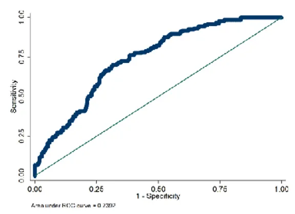
The graphical analysis is based on the models’ performance through the receiver operating characteristic (ROC) curves. These curves are related to the above-mentioned indicators: the horizontal axis is equal to one minus the specificity, while the sensitivity is represented in the vertical axis. This graphical representation allows us to quickly compare the goodness of fit of the different models. The points on the curve indicate the relation between the non-crisis observations which will be classified incorrectly by the model (horizontal axis) and the crisis observations correctly classified (vertical axis). Looking at the area under the ROC curve, or the AUROC, will give us further information on the predictive quality of the model: the larger the AUROC, the greater the predictive power of the model.
- 12 -
5. Results
In this section, we discuss the results obtained from various regressions. It includes the three different models presented in the previous chapter (Simple Probit, Dynamic Probit, and Dynamic Exuberance Probit), each with three periodic subsets (Total Period, Early Period, and Late Period).
5.1 Main Results
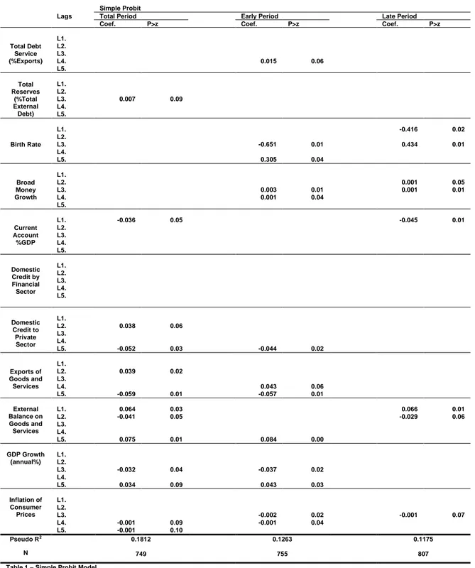
We start by analyzing the Simple Probit regressions (Table 1). Four out of the eleven selected indicators fail to show any significance when the forecasting model is based on the Total Period regression: Total Debt Service (%Exports), Birth Rate, Broad Money Growth and Domestic Credit provided by the Financial Sector. The variables Domestic Credit to Private Sector, Exports of Goods and Services, GDP Growth (annual%) and Inflation of Consumer Prices show significance for two of the five lags considered, while External Balance on Goods and Services is significant for three of the lags considered.
For the Early Period estimation, Total Debt Service (%Exports), Birth Rate and Broad Money Growth present statistically significant coefficients, in contrast with the Total Period regression. Total Reserves (% Total External Debt) and Current Account (%GDP) lose their significance. All other indicators remain significant for at least one lag, except for Domestic Credit provided by the Financial Sector, which remains non-significant.
Regarding the Late Period regression, only five indicators bare any significance: Birth Rate, Broad Money Growth, Current Account (% GDP), External Balance on Goods and Services, and Inflation of Consumer Prices.
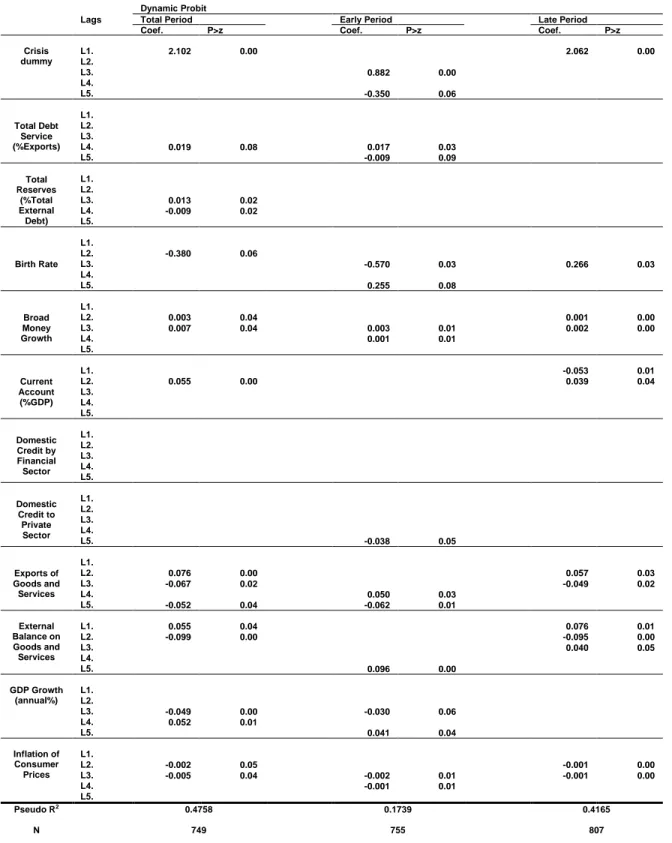
With the addition of the lagged Crisis dummy, we now analyze the Dynamic Probit model (Table 2). It is worth noticing the importance of this addition by comparing Figures 1, 2 and 3
- 13 -
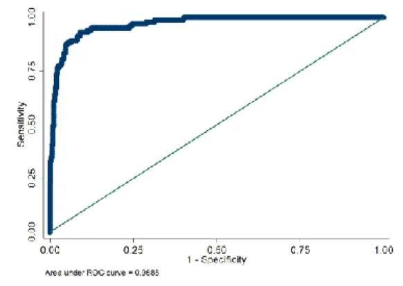
with Figures 4, 5 and 6, respectively: the ROCs move further from the 45º line, which results in higher AUROCs for the Dynamic Probit models than those obtained for the Simple Probit models. This attests to their higher predictive power and quality, achieving higher fractions of correct predictions per incorrect prediction. The lagged Crisis Dummy also proves relevant in the three sub-sets of the Dynamic Probit analysis, corroborating the narrative that crisis events are dynamic in nature.
In the Total Period regression, Exports of Goods and Services is the indicator with the highest number of significant lags, baring statistical significance two, three and five years prior to a banking crisis. Total Reserves (%Total External Debt), Broad Money Growth, External Balance on Goods and Services, GDP Growth (annual%), and Inflation of Consumer Prices show statistical significance in two lags.
Much as in the Simple Probit regression for the Early Period, Total Reserves (% Total External Debt) and Current Account (%GDP) still carry no significance for a timely forecast of a banking crisis.
In the Late Period, for the Dynamic Probit regression, we can see that External Balance on Goods and Services is a valuable indicator as it bares significance on all three lags. Birth Rate, Broad Money Growth, Current Account (%GDP), Exports of Goods and Services, and Inflation of Consumer Prices have at least one statistically significant lag in this regression, just as they did with the Simple Probit approach. Overall, Domestic Credit provided by the Financial Sector, once again, brought no significant results.
The addition of exuberance dummies to the Dynamic Probit model gives us the Dynamic
Exuberance Probit model regressions (Table 3). This allows us to evaluate whether an abnormally
large change in a variable in a given year is of added significance to forecast banking crisis episodes. Again, we can compare Figures 4, 5 and 6 from the Dynamic Probit models with Figures
- 14 -
7, 8 and 9 from the Dynamic Exuberance Probit models to confirm the benefits of this addition to
the forecasting model, which can be observed through the growth of the AUROC values.
For the Total Period Dynamic Exuberance Probit model, one indicator is statistically significant in four different lags, which deserves to be highlighted. This indicator is the Birth Rate. Inflation of Consumer Prices also stands out with three statistically significant lags. The Crisis Dummy remains highly significant and rather impactful. The most staggering result for this regression, however, relates to the exuberance factor on the Birth Rate variable, which shows statistical significance on all five years prior to a crisis event. Moreover, although Domestic Credit provided by the Financial Sector as an indicator has shown no significance in any of the regressions so far, an exuberant behavior on this variable is seemingly relevant in the Total Period forecast, carrying statistical significance in one lag.
For the Early Period model, every variable apart from Domestic Credit provided by the Financial Sector and Current Account (%GDP) is statistically significant in at least one of the three lags used.
For the Late Period, Birth Rate exuberance variables are once again of paramount importance for the forecast, by being significant in all three years preceding a banking distress. Broad Money Growth, External Balance on Goods and Services and Inflation of Consumer Prices are significant regressors on all the lags of the Late Period regression.
Comparing the Total Period forecasts between the Simple Probit, Dynamic Probit, and
Dynamic Exuberant Probit, we can see how they gradually became better with the addition of the
Crisis and Exuberance dummies. In Figure 1, the AUROC value was 0.7837. With the addition of the Crisis dummy, it grew to 0.9256 in Figure 4. Finally, after adding all the Exuberance dummies, the value reached 0.9556 in Figure 7, leaving us with a final model with a clear improvement in forecasting power. It is also worth noticing that the Late Period models perform better than the
- 15 -
Early Period models for Dynamic Probit and Dynamic Exuberance Probit models, but not for the
Simple Probit model. This may be due to the fact that the lagged Crisis Dummy is substantially
more impactful in the Late Period regression than in the Early Period regression, with larger coefficients one year prior to a banking crisis.
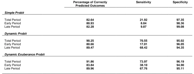
In Table 4 we can see how the percentage of correctly predicted outcomes evolves through the models. While in the Simple Probit model the highest result for this indicator was 82.64 percent in the Total Period regression, this value rose to 90.25 and 91.86 percent for the homologous regression in the Dynamic Probit and Dynamic Exuberance Probit models respectively. We can also observe that this evolution in predictive power was not due to enhanced specificity, which remained relatively stable through the models, but rather through a significant improvement in the sensitivity of the models, which shows how the successive additions to the primordial model were more relevant in correctly identifying crisis outcomes than in predicting non-crisis events. We can also see that the major difference between Late Period and Early Period models lies on this same factor, sensitivity, which is remarkably poorer in Early Period estimations.
5.2 Robustness Tests
In order to confirm the usefulness of our model and, to a certain extent, its external validity, we performed two robustness checks based on restrictions on the data used.
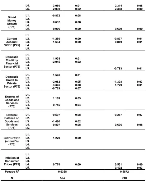
The first restriction was related to the timeframe used on the models. The period between 1979 and 1983 was plagued with banking crises all over Latin America, and most of the indicators retrieved from historical literature refer to this period. Therefore, we tested the model with the best results thus far, the Dynamic Exuberance Probit model for the Total Period, dropping from the dataset the afore-mentioned years. The results were satisfactory: with the exception of the Domestic
- 16 -
Credit variables, every indicator proved statistically significant at least one lag (Table 5), while the AUROC value rose to 0.9688 (Figure 10).
The second restricted model constructed for robustness checking was based on country exclusion. Latin America saw a number of banking crises in the 1980-90s period which could have potentially been affected by spillover effects. Thus, somewhat arbitrarily, we excluded the three Latin American countries with the highest number of banking crises between 1960 and 2014: Venezuela (which recorded 15 baking crises), Argentina and Uruguay (both counting 10 events). The results were not significantly different from the unrestricted model: the Domestic Credit variables again presented no statistically significant coefficients, and neither did the exuberance dummy variables for Exports of Goods and Services and GDP Growth (annual%). Every other variable proved statistically significant (Table 5). The AUROC value was 0.9556 (Figure 11), which is equal to the AUROC verified for the unrestricted model.
6. Concluding Remarks
The main goal of this paper was to explore the causes and indicators of banking crises in developing countries through the analysis of empirical evidence, and test the accuracy of using variables functioning as proxy to those causes when predicting a banking crisis event through a dynamic probit model.
Our results show that Birth Rate, Broad Money Growth, Exports of Goods and Services, and Inflation of Consumer Prices are the best indicators overall, giving the highest number of significant regressors across the several models. The relation between banking crises and Broad Money Growth or Inflation is clearest among these indicators, as these variables relate directly to the money supply, a direct link to the banking system. Exports of Goods and Services provide information on the well-being of a country’s economy by reflecting its competitiveness in the
- 17 -
international market. Headwinds in this front damage a country’s economic performance, which could be cause for concern among investors, thus impacting the banking system. The consistently significant results from the Birth Rate indicators corroborate the narrative that families, at least in developing countries, are influenced by the financial environment regarding the number of children they have. Thus, information on the demographic evolution of a country also seems to be helpful in predicting banking crisis events. Some indicators performed better in the early prediction models (Total Debt Service, and GDP Growth), while some were more useful for late predictions (Current Account, and External Balance on Goods and Services). Somewhat surprisingly, the variables related to credit cycles were the least informative on the probability of a banking crisis event.
Some variables were initially considered from the analysis of previous banking crises, but had to be disregarded due to scarcity of data. For instance, Interest Payment Expenses and Real Interest Rate would have been useful to further assess the impact of interest rate fluctuations; Central Government Debt, Real Effective Exchange Rate, and Global Equity Indices could have been of interest to study the influence of international market variations on the wellbeing of a country’s banking system; Life Expectancy at Birth and School Enrollment on a Tertiary Level could have contributed to further explore the relation between socio-demographic and financial variables.
Other variables related to transparency, corruption, and their ties to the financial system would have been interesting to test as leading indicators of banking crises, especially since they were so repeatedly pointed as main factors in the past. However, the data for these variables was even scarcer.
Our results also corroborate those of Antunes, Bonfim, Monteiro, & Rodrigues (2018) in the sense that the progressive additions to the Simple Probit model prove useful in enhancing the predictive power of the model, with the Dynamic Exuberance Probit model giving the best results.
- 18 -
We cannot stress enough that one of the biggest contributions of this paper comes from the intertwining of financial variations and demographical changes. Seldom used in related literature, the connection between banking distress and fluctuations in the birth rate provided one of the most consistent indicators in this study. The reasoning behind it is simple: variations in the financial environment influence the willingness of a household to add another element to the family. Further research on the matter could help clearing this link, or even test the effectiveness of other behavioral variables in forecasting banking crises.
- 19 -
7. References
▪ Amuakwa–Mensah, F., & Boakye–Adjei, A. 2015. “Determinants of non–performing loans in Ghana banking industry.” International Journal of Computational Economics and
Econometrics, 5(1): 35-54.
▪ Antunes, A., Bonfim, D., Monteiro, N., & Rodrigues, P. M. 2018. “Forecasting banking crises with dynamic panel probit models.” International Journal of Forecasting, 34(2): 249-275. ▪ Baliño, T. 1987. “The Argentine banking crisis of 1980.”
▪ Barandiarán, E., & Hernández, L. 1999. “Origins and Resolution of a Banking Crisis: Chile, 1982-86.” Banco Central de Chile.
▪ Bussiere, M., & Fratzscher, M. 2006. “Towards a new early warning system of financial crises.” Journal of International Money and Finance, 25(6): 953-973.
▪ Candelon, B., Dumitrescu, E. I., & Hurlin, C. 2014. “Currency crisis early warning systems: Why they should be dynamic.” International Journal of Forecasting, 30(4): 1016-1029. ▪ Carstens, A. G., Hardy, D. C., & Pazarbasioglu, C. 2004. “Avoiding banking crises in Latin
America.” Finance and Development, 41: 30-41.
▪ Corsetti, G., Pesenti, P., & Roubini, N. 1999. “What caused the Asian currency and financial crisis?” Japan and the world economy, 11(3): 305-373.
▪ Demirgüç-Kunt, A., & Detragiache, E. 1998. “The determinants of banking crises in developing and developed countries.” Staff Papers, 45(1): 81-109.
▪ Drehmann, M., & Juselius, M. 2012. “Improving EWIs for banking crises-satisfying policy requirements.”
▪ Edison, H. J. 2003. “Do indicators of financial crises work? An evaluation of an early warning system.” International Journal of Finance & Economics, 8(1): 11-53.
- 20 -
▪ García-Herrero, M. A. 1997. “Banking Crises in Latin America in the 1990's: Lessons From Argentina, Paraguay, and Venezuela.” International Monetary Fund.
▪ Goldstein, I., & Razin, A. 2013. “Review of theories of financial crises.” National Bureau of
Economic Research.
▪ Griffith-Jones, S. 1998. “Causes and lessons of the Mexican Peso crisis.” In Global Capital
Flows, 100-136.
▪ Honohan, P. 1997. “Banking system failures in developing and transition countries: Diagnosis and predictions.”
▪ Kaminsky, G. L., & Reinhart, C. M. 1998. “Financial crises in Asia and Latin America: Then and now.” The American Economic Review, 88(2): 444-448.
▪ Kaminsky, G., Lizondo, S., & Reinhart, C. M. 1998. “Leading indicators of currency crises.” Staff Papers, 45(1): 1-48.
▪ Kauppi, H., & Saikkonen, P. 2008. “Predicting US recessions with dynamic binary response models.” The Review of Economics and Statistics, 90(4): 777-791.
▪ Lopes, A. M., Machado, J. T., Huffstot, J. S., & Mata, M. E. 2018. “Dynamical analysis of the global business-cycle synchronization.” PloS one, 13(2).
▪ Sanusi, L. S. 2010. “The Nigerian Banking Industry: what went wrong and the way forward.” Delivered at Annual Convocation Ceremony of Bayero University, Kano.
- 21 -
8. Appendix
8.1 Tables
Simple Probit
Lags Total Period Early Period Late Period
Coef. P>z Coef. P>z Coef. P>z
Total Debt Service (%Exports) L1. L2. L3. L4. 0.015 0.06 L5. Total Reserves (%Total External Debt) L1. L2. L3. 0.007 0.09 L4. L5. Birth Rate L1. -0.416 0.02 L2. L3. -0.651 0.01 0.434 0.01 L4. L5. 0.305 0.04 Broad Money Growth L1. L2. 0.001 0.05 L3. 0.003 0.01 0.001 0.01 L4. 0.001 0.04 L5. Current Account %GDP L1. -0.036 0.05 -0.045 0.01 L2. L3. L4. L5. Domestic Credit by Financial Sector L1. L2. L3. L4. L5. Domestic Credit to Private Sector L1. L2. 0.038 0.06 L3. L4. L5. -0.052 0.03 -0.044 0.02 Exports of Goods and Services L1. L2. 0.039 0.02 L3. L4. 0.043 0.06 L5. -0.059 0.01 -0.057 0.01 External Balance on Goods and Services L1. 0.064 0.03 0.066 0.01 L2. -0.041 0.05 -0.029 0.06 L3. L4. L5. 0.075 0.01 0.084 0.00 GDP Growth (annual%) L1. L2. L3. -0.032 0.04 -0.037 0.02 L4. L5. 0.034 0.09 0.043 0.03 Inflation of Consumer Prices L1. L2. L3. -0.002 0.02 -0.001 0.07 L4. -0.001 0.09 -0.001 0.04 L5. -0.001 0.10 Pseudo R2 0.1812 749 0.1263 755 0.1175 807 N
Table 1 – Simple Probit Model
- 22 -
Dynamic Probit
Lags Total Period Early Period Late Period
Coef. P>z Coef. P>z Coef. P>z
Crisis dummy L1. 2.102 0.00 2.062 0.00 L2. L3. 0.882 0.00 L4. L5. -0.350 0.06 Total Debt Service (%Exports) L1. L2. L3. L4. 0.019 0.08 0.017 0.03 L5. -0.009 0.09 Total Reserves (%Total External Debt) L1. L2. L3. 0.013 0.02 L4. -0.009 0.02 L5. Birth Rate L1. L2. -0.380 0.06 L3. -0.570 0.03 0.266 0.03 L4. L5. 0.255 0.08 Broad Money Growth L1. L2. 0.003 0.04 0.001 0.00 L3. 0.007 0.04 0.003 0.01 0.002 0.00 L4. 0.001 0.01 L5. Current Account (%GDP) L1. -0.053 0.01 L2. 0.055 0.00 0.039 0.04 L3. L4. L5. Domestic Credit by Financial Sector L1. L2. L3. L4. L5. Domestic Credit to Private Sector L1. L2. L3. L4. L5. -0.038 0.05 Exports of Goods and Services L1. L2. 0.076 0.00 0.057 0.03 L3. -0.067 0.02 -0.049 0.02 L4. 0.050 0.03 L5. -0.052 0.04 -0.062 0.01 External Balance on Goods and Services L1. 0.055 0.04 0.076 0.01 L2. -0.099 0.00 -0.095 0.00 L3. 0.040 0.05 L4. L5. 0.096 0.00 GDP Growth (annual%) L1. L2. L3. -0.049 0.00 -0.030 0.06 L4. 0.052 0.01 L5. 0.041 0.04 Inflation of Consumer Prices L1. L2. -0.002 0.05 -0.001 0.00 L3. -0.005 0.04 -0.002 0.01 -0.001 0.00 L4. -0.001 0.01 L5. Pseudo R2 0.4758 749 0.1739 755 0.4165 807 N
Table 2 – Dynamic Probit Model
- 23 -
Dynamic Exuberance Probit
Lags Total Period Early Period Late Period
Coef. P>z Coef. P>z Coef. P>z
Crisis dummy L1. 2.515 0.00 2.118 0.00 L2. L3. 0.763 0.00 L4. L5. -0.342 0.03 Total Debt Service (%Exports) L1. L2. L3. L4. 0.025 0.05 0.018 0.07 L5. -0.037 0.01 -0.026 0.02 Total Reserves (%Total External Debt) L1. L2. L3. 0.003 0.08 L4. -0.010 0.07 L5. Birth Rate L1. 0.115 0.09 L2. -0.543 0.01 L3. -0.607 0.07 0.345 0.00 L4. -0.127 0.08 L5. 0.388 0.00 0.244 0.01 Broad Money Growth L1. -0.001 0.01 L2. 0.005 0.00 0.001 0.00 L3. 0.002 0.01 0.001 0.02 L4. 0.003 0.01 L5. Current Account %GDP L1. -0.057 0.01 L2. 0.111 0.01 0.067 0.03 L3. L4. L5. Domestic Credit by Financial Sector L1. L2. L3. L4. L5. Domestic Credit to Private Sector L1. L2. L3. L4. L5. -0.040 0.07 Exports of Goods and Services L1. L2. 0.089 0.00 0.059 0.05 L3. -0.096 0.00 -0.054 0.02 L4. 0.056 0.02 L5. -0.055 0.00 External Balance on Goods and Services L1. 0.096 0.01 0.094 0.00 L2. -0.128 0.00 -0.111 0.00 L3. 0.051 0.03 L4. L5. 0.094 0.01 GDP Growth (annual%) L1. L2. L3. L4. 0.100 0.00 L5. 0.077 0.01 Inflation of Consumer Prices L1. 0.001 0.01 L2. -0.003 0.00 -0.001 0.01 L3. -0.006 0.02 -0.002 0.01 -0.001 0.02 L4. -0.002 0.01 L5. Total Debt Service (%Exports) (P75) L1. L2. 0.545 0.09 L3. L4. L5. Total Reserves (%Total External Debt) (P75) L1. L2. L3. -0.815 0.02 -0.772 0.03 -0.453 0.00 L4. L5. Birth Rate (P75) L1. 1.283 0.01 0.699 0.04 L2. 4.423 0.00 3.248 0.00 L3. -5.214 0.00 -3.931 0.00
- 24 - L4. 2.315 0.07 2.302 0.01 L5. -2.369 0.00 -3.293 0.00 Broad Money Growth (P75) L1. L2. L3. 0.344 0.06 L4. L5. 0.610 0.00 0.315 0.10 Current Account %GDP (P75) L1. L2. -0.838 0.01 L3. 0.849 0.01 0.621 0.01 L4. L5. Domestic Credit by Financial Sector (P75) L1. L2. L3. -0.612 0.09 L4. L5. -0.782 0.01 Domestic Credit to Private Sector (P75) L1. L2. L3. -1.303 0.03 L4. 1.729 0.01 L5. Exports of Goods and Services (P75) L1. L2. L3. 0.295 0.09 L4. L5. External Balance on Goods and Services (P75) L1. -0.287 0.07 -0.383 0.01 L2. L3. -0.798 0.00 -0.499 0.08 L4. 0.636 0.08 L5. GDP Growth (annual%) (P75) L1. L2. L3. L4. L5. -0.398 0.09 Inflation of Consumer Prices (P75) L1. L2. L3. 0.437 0.01 L4. 0.531 0.00 0.356 0.00 L5. 0.402 0.03 0.585 0.00 Pseudo R2 0.5875 749 0.2890 755 0.4753 807 N
Table 3 – Dynamic Exuberance Model
The total period refers to lags [5;1], the early period to lags [5;3] and the late period to lags [3;1]. Standard errors are clustered by country.
Percentage of Correctly Predicted Outcomes Sensitivity Specificity Simple Probit Total Period 82.64 21.92 97.35 Early Period 80.93 8.84 98.36 Late Period 82.28 9.87 99.08 Dynamic Probit Total Period 90.25 70.55 95.02 Early Period 80.66 17.01 96.05 Late Period 89.47 68.42 94.35
Dynamic Exuberance Probit
Total Period 91.86 73.97 96.19
Early Period 83.84 38.10 94.90
Late Period 89.96 67.76 95.11
- 25 -
Dynamic Exuberance Probit – Robustness Checks, Total Period
Lags Year Restricted Country Restricted
Coef. P>z Coef. P>z Crisis dummy L1. 2.624 0.00 2.514 0.00 L2. L3. L4. L5. Total Debt Service (%Exports) L1. 0.057 0.00 L2. -0.054 0.03 L3. L4. 0.025 0.05 L5. -0.058 0.00 -0.037 0.01 Total Reserves (%Total External Debt) L1. L2. L3. L4. -0.013 0.05 -0.010 0.07 L5. 0.007 0.05 Birth Rate L1. 0.275 0.01 0.115 0.09 L2. -1.228 0.00 -0.542 0.01 L3. 0.541 0.00 L4. -0.275 0.00 -0.127 0.08 L5. 0.729 0.00 0.388 0.00 Broad Money Growth L1. L2. 0.006 0.00 0.005 0.00 L3. 0.003 0.00 L4. 0.003 0.00 0.003 0.01 L5. Current Account %GDP L1. L2. 0.174 0.00 0.111 0.01 L3. -0.090 0.09 L4. L5. Domestic Credit by Financial Sector L1. L2. L3. L4. L5. Domestic Credit to Private Sector L1. L2. L3. L4. L5. Exports of Goods and Services L1. L2. 0.089 0.00 L3. -0.125 0.00 -0.096 0.00 L4. 0.075 0.03 L5. -0.069 0.02 External Balance on Goods and Services L1. 0.120 0.00 0.096 0.01 L2. -0.173 0.01 -0.128 0.00 L3. L4. L5. GDP Growth (annual%) L1. L2. -0.127 0.00 L3. -0.102 0.05 L4. 0.104 0.02 0.100 0.00 L5. Inflation of Consumer Prices L1. L2. -0.005 0.00 -0.003 0.00 L3. -0.002 0.02 -0.006 0.02 L4. -0.002 0.00 -0.002 0.01 L5. -0.002 0.01 Total Debt Service (%Exports) (P75) L1. -0.737 0.01 L2. 0.785 0.06 0.545 0.09 L3. L4. L5. 1.093 0.00 Total Reserves (%Total External Debt) (P75) L1. L2. L3. -1.312 0.00 -0.814 0.02 L4. 1.039 0.04 L5. -0.720 0.09 Birth Rate (P75) L1. -2.265 0.07 1.282 0.01 L2. 9.806 0.00 4.421 0.00 L3. -7.895 0.00 -5.212 0.00
- 26 - L4. 3.060 0.01 2.314 0.08 L5. -2.039 0.02 -2.368 0.00 Broad Money Growth (P75) L1. -0.872 0.08 L2. L3. 0.632 0.08 L4. L5. 0.906 0.00 0.609 0.00 Current Account %GDP (P75) L1. L2. -1.250 0.00 -0.837 0.01 L3. 1.634 0.00 0.849 0.01 L4. L5. Domestic Credit by Financial Sector (P75) L1. L2. 1.938 0.01 L3. -2.045 0.02 L4. L5. -0.783 0.01 Domestic Credit to Private Sector (P75) L1. 1.546 0.01 L2. L3. -2.062 0.05 -1.303 0.03 L4. 3.346 0.00 1.729 0.01 L5. -0.729 0.07 Exports of Goods and Services (P75) L1. L2. 1.109 0.03 L3. L4. -0.755 0.04 L5. External Balance on Goods and Services (P75) L1. -0.597 0.08 -0.287 0.07 L2. L3. -1.490 0.02 L4. 0.807 0.08 0.636 0.08 L5. GDP Growth (annual%) (P75) L1. L2. 1.220 0.00 L3. L4. L5. Inflation of Consumer Prices (P75) L1. L2. L3. L4. 0.774 0.00 0.531 0.00 L5. 0.402 0.03 Pseudo R2 0.6358 594 0.5872 748 N
Table 5 – Robustness Check Models
The total period refers to lags [5;1], the early period to lags [5;3] and the late period to lags [3;1]. Standard errors are clustered by country.
- 27 -
8.2 Figures
Figure 1 - Simple Probit Model, Total Period Figure 2 - Simple Probit Model, Early Period
Figure 3 - Simple Probit Model, Late Period Figure 4 - Dynamic Probit Model, Total Period
- 28 -
Figure 7 - Dynamic Exuberance Probit Model, Total Period
Figure 8 - Dynamic Exuberance Probit Model, Early Period
Figure 9 - Dynamic Exuberance Probit Model, Late Period Figure 10 - Dynamic Probit Exuberance Model, Robustness Test on Years
Figure 11 - Dynamic Exuberance Probit Model, Robustness Test on Countries