A New Approach to Monte Carlo Simulations in Statistical Physics
D. P. Landau
1and F. Wang
21Center for Simulational Physics, The University of Georgia, Athens, GA 30602, USA
2Paracer Inc., 1371 Shorebird Way Mountain View, CA 94043, USA
Received on 5 September, 2003
We describe a new algorithm that approaches Monte Carlo simulation in statistical physics in a different way. Instead of sampling the probability distribution at a fixed temperature, a random walk is performed in energy space to directly extract an estimate for the density of states. The canonical probability can then be found at any temperature by weighting by the appropriate Boltzmann factor, and thermodynamic properties can be determined from suitable derivatives of the partition function.
1
Introduction
During the last half of the 20th century great strides were made in the theoretical and experimental investigation of condensed matter systems, and consequently our under-standing of phase transitions was dramatically enhanced. Certain problems remained, however,in part because imper-fections in physical systems limited the resolution of exper-iment and in part because analytical solutions of all but the simplest theoretical models proved elusive. Computer sim-ulation now plays a significant role in statistical physics [1], particularly for the study of phase transitions and critical phenomena. The “standard” Monte Carlo method, which is flexible and easy to implement, has been the Metropolis importance sampling algorithm [2], but near phase transi-tions this method becomes inefficient because of the long time scales that develop. A number of more efficient algo-rithms have now been introduced to circumvent this prob-lem, but these are somewhat limited in applicability. Begin-ning with the seminal work of Swendsen and Wang [3] and extended by Wolff [4], cluster flipping algorithms have been used to reduce critical slowing down near 2nd order tran-sitions. An approach which is quite different in spirit, the multicanonical ensemble method [5-8], was introduced to overcome the tunneling barrier between coexisting phases at 1st order transitions and has general utility for systems with a rough energy landscape [7-17]. In all cases, histogram reweighting techniques [18] can be applied in the analysis to increase the amount of information that can be gleaned from simulational data, but the applicability of reweighting is severely limited in large systems by the statistical qual-ity of the “wings” of the histogram. This latter effect is quite limiting in systems with frustration that produces a very complicated energy landscape and limits the efficiency of “standard” methods.
The partition function of any model can be expressed in terms of a density of states g(E), i.e. the number of all possible states(or configurations) for an energy levelE
of the system, but direct estimation of this quantity has not
been the goal of simulations. Instead, most conventional Monte Carlo algorithms [1], such as Metropolis importance sampling, Swendsen-Wang cluster flipping, etc. generate a canonical distributiong(E)e−E/kBT at a given temperature.
Such distributions are so narrow that multiple runs are usu-ally needed to describe thermodynamic quantities over a sig-nificant range of temperature. In the canonical distribution,
g(E)does not depend on the temperature and knowledge of
g(E)permits construction of canonical distributions at any temperature. (Onceg(E)is known the partition functionZ
can be calculated:
Z=
{configurations}
e−βE=
E
g(E)e−βE, (1)
whereβ = 1/(kBT), and the model is essentially “solved”
since most thermodynamic quantities can be extracted from it.)
Even though Monte Carlo methods are already very powerful [1], there was no efficient algorithm to calculate
g(E)very accurately for large systems. Even for exactly solvable models such as the 2-dim Ising model,g(E) can-not be calculated exactly for a large system [19]. All meth-ods based on accumulation of histogram entries, such as the histogram method of Ferrenberg and Swendsen [18] , Lee’s version of the multicanonical method(entropic sam-pling) [20], the broad histogram method [21-24] and flat histogram method [25] have the problem of scalability for large systems. Thus, an algorithm is still needed to calculate the density of states for large systems.
We now describe a simple new, general, and efficient Monte Carlo algorithm (generally known as “Wang-Landau sampling”) that offers substantial advantages over existing approaches [29-31]. Unlike conventional Monte Carlo methods that generate a canonical distribution at a given temperature g(E)e−E/kBT, this approach estimates g(E)
controlled modification factor, to produce a result that con-verges to the correct value very quickly. The thermodynamic quantities can then be extracted by applying canonical aver-age formulas in statistical physics.
2
The “Wang-Landau” algorithm
“Wang-Landau sampling” is based on the observation that if we perform a random walk in energy space by flipping spins randomly for a spin system, and the probability to visit a given energy levelEis proportional to the reciprocal of the density of states g(1E), then a flat histogram is generated for the energy distribution. This is accomplished by modify-ing the estimated density of states in a systematic way to produce a “flat” histogram over the allowed range of energy and simultaneously makingg(E)converge to the true value.
g(E)is modified constantly during each step of the random walk and use the updated density of states to perform a fur-ther random walk in energy space. The modification factorf
is controlled carefully, and at the end of simulation it should be very close to1which is the ideal case of the random walk with the true density of states.
Initially,g(E)isa prioriunknown, so the simplest ap-proach is to set all entries tog(E) = 1for all possible en-ergiesE. Then a random walk in energy space is begun by flipping spins randomly with the probability at a given en-ergy level proportional to g(1E). IfE1andE2are energies before and after a spin is flipped, the transition probability from energy levelE1toE2is:
p(E1→E2) = min(
g(E1)
g(E2),1).
(2) Each time an energy levelEis visited, the existing value is multiplied by the modification factorf > 1, i.e. g(E) →
g(E) ∗ f. (It is preferable to work with the logarithm i.e.ln(g(E))→ln(g(E)) + ln(f)so that all possibleg(E) will fit into double precision numbers.) If the random walk rejects a trial move, g(E) is also modified with the same modification factor. A reasonable, although not necessarily optimal, choice of the initial modification factor isf =f0=
e1≃2.71828...which allowsg(E)to develop rapidly. Iff0 is too small, the random walk will take too long to reach all possible energies; however, large statistical errors result iff0 is too large. During the random walk, the histogramH(E) (the number of visits at each energy levelE) is accumulated; and when it is approximately flat, the density of states will have converged to the true value with an accuracy propor-tional to that modification factor ln(f). The modification factor is then reduced e.g. f1 = √f0, the histogram is re-zeroed, and a new random walk is begun. This iterative pro-cedure continues until the modification factor is smaller than a predefined value (e.g.ffinal= exp(10−8)≃1.00000001).
The modification factor acts as a control parameter for the accuracy ofg(E)during the simulation and also determines how many MC sweeps are necessary for the entire simula-tion. It is impossible to obtain a perfectly flat histogram and the phrase “flat histogram” that all histogram entries are not less thanx%of the average histogramH(E), wherex%is
chosen according to the size and complexity of system and the desired accuracy ofg(E).
Clearly, one essential constraint is thatg(E)should con-verge to the true value. The accuracy of the estimate for
g(E) is proportional to ln(f) at that iteration; however, ln(ffinal)can not be chosen arbitrarily small or the modified
ln(g(E))will not differ from the unmodified one to within the number of digits in the double precision numbers used in the calculation. If this happens, the algorithm no longer converges to the true value, and the program may run for-ever. Evenffinalis within range, but too small, the
calcula-tion might take excessively long.
The method can be further enhanced by performing mul-tiple random walks, each for a different range of energy, ei-ther serially or in parallel fashion, with the random walk re-stricted to remain in the desired range. The resultant pieces ofg(E) can then be joined together and used to produce canonical averages for the calculation of thermodynamic quantities at any temperature.
Note that the algorithm does not satisfy the detailed bal-ance condition exactly (especially for early stages of itera-tion) sinceg(E)is modified constantly during the random walk. However, after many iterations it quickly converges to the true value asf →1. Ifp(E1→E2)is the transition probability from energy levelE1to levelE2, from Eqn. (2), the ratio of the transition probabilities fromE1 toE2 and fromE2toE1is:
p(E1→E2)
p(E2→E1) =
g(E1)
g(E2)
(3) whereg(E)is the density of states. In another words, the random walk algorithm satisfies detailed balance:
1
g(E1)
p(E1→E2) = 1
g(E2)
p(E2→E1) (4) where g(E1
1) is the probability at the energy level E1 and
p(E1 → E2)is the transition probability from E1 toE2 for the random walk. We conclude that the detailed balance condition is satisfied with accuracy proportional to the mod-ification factorln(f).
Almost all recursive methods updateg(E)by using the histogram data directly only after enough histogram entries are accumulated [5, 8, 11, 13, 14, 15, 16, 27, 32, 33, 34]. Because of the exponential growth ofg(E)in energy space, this process is inefficient because the histogram is accumu-lated linearly. Instead, we modifyg(E)at each step of the random walk, and this allows us the approach to the true distribution to be much faster than conventional methods, especially for large systems. (Although histogram entries are accumulated during the random walk, they are only used to check if the histogram is flat enough to go to the next level iteration.)
is about2N, whereN = L2 is the total number of lattice sites. In contrast, the average number of possible states for each energy level is as large as q2NN, whereqN is the total
number of possible configurations of the system. Clearly, current computers are unable to realize all possible states to calculate any thermodynamic quantities even though most models in statistical physics are well defined. This is also why efficient and fast simulational algorithms are required in the numerical investigations.
With the density of states, we not only can calculate most of thermodynamic quantities in all temperature region with-out multiple simulations but can also access some quantities, such as the free energy and entropy, which are not directly available from conventional Monte Carlo simulations. The free energy is calculated using
F =−kTlog(Z) (5) All other thermodynamic properties can also be calculated from the density of states, e.g. the internal energy is given by:
U(T) =
E
Eg(E)e−βE
E
g(E)e−βE ≡ ET (6)
and the specific heat can be estimated from the fluctuations in the internal energy:
C(T) = ∂U(T)
∂T =
E2
T − ET2
T2 . (7) Thus, a single simulation should be sufficient to provide all interesting information about a system.
3
How well does the method work?
3.1
Application to the Ising square lattice
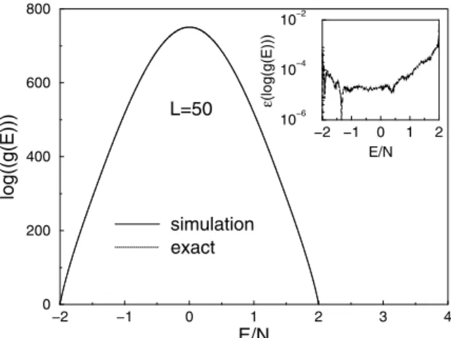
As a test of the accuracy and convergence of the method, we apply it first toL×LIsing square lattices with nearest neigh-bor coupling. Not only is the Ising model the “fruit fly” of statistical mechanics but so many of its properties can be de-termined exactly so a truly quantitative check of the method is possible (see e.g. Ref. [37]). The exact solution for the partition function for finite-size systems [38] provides information about thermodynamic properties. Using Math-ematica the exact density of states can be obtained for small systems [19], and we extended the calculation up toL= 50 with the Mathematica program provided by Beale. With the algorithm described here,g(E)was estimated for the Ising model forL = 50, with the final modification factor be-ing1.000000001, and these results are compared with exact values in Fig. 3.1. To within the resolution of the figure, simulational data and the exact solution overlap perfectly, so in the inset we show the relative error:
ε(X)≡ |XsimX−Xexact|
exact
(8)
Over most of the region ε(log(g)) is smaller than 0.01%. Such errors for low energy levels are directly related to the errors for the thermodynamic quantities calculated from the density of states. The average relative error is 0.019% for
L= 50. In comparison, a recent broad histogram study of a 2D Ising model on a32×32lattice [24] yielded an average deviation of the microcanonical entropy that was substan-tially larger than that from this random walk algorithm.
−2 −1 0 1 2 3 4
E/N
0 200 400 600 800
log((g(E)))
simulation exact
−2 −1 0 1 2
E/N
10−6
10−4
10−2
ε
(log(g(E)))
L=50
Figure 1. Density of states for theL= 50Ising square lattice with
periodic boundary conditions (pbc).
The normalized density of states in Fig. 1 is obtained by normalizing to the condition that the number of ground states is 2 (i.e. all up or all down).
For very large values of L we can divide the desired energy region [-2, 0.2] into multiple energy segments and estimate the density of states on each segment with an in-dependent random walk. The resultant density of states can be joined from adjacent energy segments. A compari-son of thermodynamic properties determined in overlapping ranges of energy showed that data are actually only needed over restricted ranges, e.g. results for three independent ran-dom walks performed in the rangesE/N = [−1.7,−1.2],
E/N = [−1.8,−1.1]andE/N = [−1.9,−1.0]showed no discernable difference to the temperature dependence near the phase transition. Boundary effects at the edges of the en-ergy ranges can be eliminated by simply treating spin flips that are rejected because the new energy would be out of range in the same manner as any rejected spin-flip.
Since the exact g(E) is only available for small systems(L ≤ 50), it is also important to test the accuracy of estimates for thermodynamic quantities of large systems. Using canonical average formulas to calculate internal en-ergy, specific heat, Gibbs free energy and entropy. Ferdi-nand and Fisher [38] the exact solutions of above quantities for 2D Ising model on finite-size lattices can be compared with simulational results.
shows the relative errorsε(S)ForL= 256the relative er-ror is smaller than0.1%over almost the entire temperature range.
0 2 4 6 8
T
0 0.2 0.4 0.6 0.8
S(T)/N
simulation exact
0 2 4 6 8
T
10−6
10−4
10−2
100
ε
(S)
256x256 Ising model
(a)
2.1 2.2 2.3 2.4
T
1 1.5 2 2.5 3
C(T)
simulation exact
0 2 4 6 8
T
0 0.02 0.04
ε
(C)
L=256
L=128
L=64 L=256
(b)
Figure 2. Thermodynamic properties of the Ising square lattice with pbc: (a)Entropy; (b)Specific heat.
g(E)can also be used to calculate the specific heat as a function of temperature. Both simulational data and exact results nearTcare shown in Fig. 2(b) forL = 64, 128 and
256 Ising model. To within the error bars there is no differ-ence between the simulational data and exact solutions. In the inset of Fig. 2(b), we show relative errors as a function of temperature for L = 256. The errors for specific heat for a 256×256lattice are smaller than 4.5%for all tem-peratures. Recently, Wanget al.[36] estimated the specific heat of the same model on a64×64lattice by the transi-tion matrix Monte Carlo re-weighting method [39], and for a simulation with2.5×107MC sweeps, the maximum error in temperature regionT ∈ [0,8]was about 1%. When we apply this algorithm to the same model on the64×64 lat-tice, with a final modification factor of1.000000001and a total of2×107MC sweeps on single processor, the errors in the specific heat are reduced below 0.7% for all temperature. The relatively large errors at lowT reflect the small values for the specific heat.
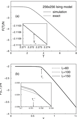
The behavior of the free energy nearTccannot be
ex-tracted from “standard” Monte Carlo simulations but can be straightforwardly found from g(E) using Eqn.(5). In Fig. 3(a), the simulational data and exact results are
pre-sented in the same figure. To within the resolution of the figure, no difference is visible, and the relative errors are smaller than0.001%for all temperatures.
0 2 4 6 8
T
−6 −5 −4 −3 −2
F(T)/N
simulation exact
2.271 2.272 2.273 2.274
−2.1112 −2.1109 −2.1106 −2.1103
256x256 Ising model
Tc (a)
0 0.5 1 1.5
T
−4 −3.5 −3 −2.5 −2
F(L,T)/N
L=60 L=100 L=150
0.7 0.701 0.702 0.703
−2.036 −2.034 −2.032
Tc
Tc
∞ (b)
Figure 3. (a)Free energy of the Ising square lattice; (b)Free energy of theq= 10Potts model.
3.2
Application to the
q
= 10
Potts model: A
first order phase transition
In this section, we show how the algorithm is well suited to the study of a model with a strong first-order phase transi-tion [40, 41]. In such cases, the internal energy, entropy, etc. have discontinuities at the transition and both ordered and disordered states coexist at the transition. We choose the two-dimensional, ten state Potts model since it has a strong temperature-driven first-order phase transitions and a great deal is know about its behavior. We consider the Potts model onL×Lsquare lattices with nearest-neighbor interactions and periodic boundary conditions. The Hamiltonian for this model can be written as:
H =−
<ij>
δ(qi, qj) (9)
andq = 1,2, ...q. During the simulation, we select lattice sites randomly and choose integers between[1 : q] ran-domly for new Potts spin values. The modification factor
ffinal= exp(10−8)≃1.00000001by the end of the random
walk. At the end of the simulations,g(E)is normalized us-ing the fact that the total number of possible states isqN or
that the number of ground states isq, whereN =L2is the total number of lattice sites. (Actually one of these two con-ditions can be used to get the absolute density of states and the other condition to check the accuracy of the result.) To guarantee the accuracy of thermodynamic quantities at low temperatures, we use the condition that the number of the ground states isqto normalize the density of states.
Conventional Monte Carlo simulation (e.g. Metropo-lis sampling [1, 2]) determines the canonical distribution
P(E, T)by generating a random walk Markov chain at a given temperature:
P(E, T) =g(E)e−E/kBT (10)
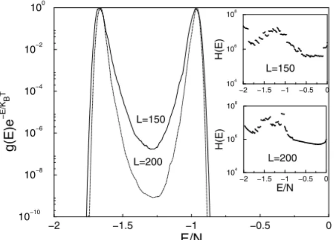
From the simulational result forg(E), we can calculate the canonical distribution by the above formula at essentially any temperature without performing multiple simulations. In Fig. 4 we show the resultant double peaked canonical dis-tribution [41], at the transition temperatureTcfor the
first-order transition of the q = 10 Potts model. The “transi-tion temperatures”Tc(L) are determined by the
tempera-tures where the double peaks are of the same height. (Note that the peaks of the distributions are normalized to 1 in this figure.) The valley between two peaks is quite deep. e.g. is 10−9forL= 100. The latent heat for this temperature driven first-order phase transition can be estimated from the energy difference between the double peaks. Our results for the locations of the peaks are consistent with the results ob-tained by multicanonical method [6] and multibondic clus-ter algorithm [7] for those lattice sizes for which these other methods are able to generate estimates. Wang-Landau sam-pling also produces results for substantially larger systems than have been studied by these other approaches.
−2 −1.5 −1 −0.5 0
E/N
10−10
10−8
10−6
10−4
10−2
100
g(E)e
−E/K
B
T
−2 −1.5 −1 −0.5 0
E/N
104
106
108
H(E)
−2 −1.5 −1 −0.5 0
104
106
108
H(E)
L=150
L=200
L=150
L=200
Figure 4. Canonical probability for theq= 10Potts square lattice with periodic boundary conditions.
Because of the double peak structure at a first-order phase transition, conventional Monte Carlo simulations are not efficient since an extremely long time is required for the system to travel from one peak to the other in energy space. With “Wang-Landau sampling” all possible energy
levels are visited with equal probability, so it overcomes the tunneling barrier between the coexisting phases in the con-ventional Monte Carlo simulations.
If we are only interested in a specific temperature range, e.g. nearTc, we could first perform a low precision
unre-stricted random walk, i.e. over all energies, to estimate the required energy range, and then carry out a very accurate random walk for the corresponding energy region. The in-set of Fig. 4 only shows the histograms for the extensive random walks in the energy range betweenE/N =−1.90 and−0.6. If we need to know the density of states more accurately for some energies, we also can perform separate simulations, one for low energy levels, one for high energy levels, the other for middle energy which includes double peaks of the canonical distribution atTc. This scheme not
only speeds up the simulation, but also increases the prob-ability of accessing the energy levels for which both maxi-mum and minimaxi-mum values of the distributions occur by per-forming the random walk in a relatively small energy range. If we perform single random walk over all possible energies, it will take a long time to generate rare spin configurations. Such rare energy levels include the ground energy level or low energy levels with only few spins with different values and high energy levels where all, or most, adjacent Potts spins have different values.
If the system is not larger than100×100, the random walk in important energy regions (i.e. that which includes the two peaks of the canonical distribution atTc) can be
car-ried out efficiently with a single processor. However, for a larger system it is advisable to accelerate the calculation by performing random walks in different energy regions, each using a different processor. The densities of states for 150×150and200×200, shown in Fig. 4, were obtained by joining together the estimates obtained from21 indepen-dent random walks, each constrained within a different re-gions of energy. The histograms from the individual random walks are shown in the inset of Fig. 4 both for 150×150 and200×200lattices. In this case, we only require that the histogram of the random walk in the corresponding en-ergy segment is sufficiently flat without regard to the relative flatness over the entire energy range. The probability distri-butions for large lattices show pronounced double peaks for the canonical distributions at temperaturesTc(L) = 0.70127
forL= 150andTc(L) = 0.701243forL= 200. The exact
result isTc = 0.701232....for the infinite system.
Consid-ering the minimum forL= 200is as deep as10−9, we can understand why is impossible for conventional Monte Carlo algorithms to overcome the tunneling barrier with available computational resources.
To check the accuracy of the results we can estimate the transition temperature of theq= 10Potts model forL=∞ since the exact solution is known. According to finite-size scaling theory, the “effective” transition temperature for fi-nite systems behaves as:
Tc(L) =Tc(∞) +
c
Ld (11)
whereTc(L)andTc(∞)are the transition temperatures for
The transition temperature varies asL−d and the
tran-sition temperature extrapolated from our simulational data is consistent with the exact solution for the infinite system. We also compared our results with the existing numerical data such as estimates of transition temperatures and dou-ble peak locations obtained with the multicanonical simula-tional method by Berg and Neuhaus [5] and the Multibondic cluster algorithm by Janke and Kappler [7]. With the ran-dom walk simulational algorithm, we can calculate the den-sity of states up to200×200within107visits per energy level to obtain a good estimate of the transition temperature and locations of the double peaks. Using the multicanonical method and a finite scaling guess for the density of states, Berg et. al. only obtained results for lattices as large as 100×100[5], and multibondic cluster algorithm data [7] were not given for systems larger than50×50.
When we calculate the internal energy near the transi-tion, we find that a very sharp “jump” appears in the internal energy atTc. The magnitude of this jump equals the latent
heat for the (first-order) phase transition and is related to the double peak distribution of the first-order phase transition. WhenTis slightly different thanTc, one of the double peaks
increases dramatically in magnitude and the other decreases. Since we only perform simulations on finite lattices, and use a continuous function to calculate thermodynamic quanti-ties, all our quantities for finite-size systems will appear to be continuous if we use a very small scale. The same density of states can be used to calculate the internal energy for tem-peratures very close toTc. On this scale the “discontinuity”
at the first-order phase transition disappears and a smooth curve can be seen instead of a sharp “jump”. When the sys-tem size goes to infinity, the discontinuity will be real.
The specific heat in the vicinity of the transition temper-atureTcshows pronounced finite size behavior. We find it
has a finite maximum value for a given lattice sizeLthat, according to finite-size scaling theory for first-order transi-tions, should vary as:
c(L, T)L−d∝f((T−T
c(∞)Ld) (12)
wherec(L, T) =C(L, T)/Nis the specific heat per lattice site,Lis the linear lattice size,d= 2is the dimension of the lattice. T(L = ∞) = 0.70123....is the exact solution for theQ= 10Potts model [35]. Indeed, the simulational data for systems with L = 60,100and200can be well fitted by a single scaling function, moreover this function is com-pletely consistent with the one obtained from lattice sizes fromL= 18toL= 50by standard Monte Carlo [41].
The results for the free energy per lattice site are shown in Fig. 3(b) as a function of temperature. Since the transition is first-order the free energy appears to have a “discontinu-ity” in the first derivative atTc. This is typical behavior for a
first-order phase transition, and even with the fine scale used in the inset of Fig. 3(b), this property is still apparent even though the system is finite. The transition temperatureTcis
determined by the point where the first derivative appears to be discontinuous. With a coarse temperature scale we can not distinguish the finite-size behavior of our model; how-ever, we can see a very clear size dependence when we view the free energy on a very fine scale as in the inset.
The entropy is another very important thermodynamic quantity that cannot be calculated directly in conventional Monte Carlo simulations. It can be estimated by integrating over other thermodynamic quantities, such as specific heat, but the result is not always reliable since the specific heat itself is not easy to determine accurately, particularly con-sidering the “divergence” at the first-order transition. With an accurate density of states estimated by our method, we already know the Gibbs free energy and internal energy for the system, so the entropy can be calculated easily:
S(T) =U(T)−F(T)
T (13)
It is very clear that the entropy is very small at low temper-ature and atT = 0is given by the density of states for the ground states. The entropy has a very sharp “jump” atTc,
just as does the internal energy, and this is easily visible in a plot of the entropy nearTc. The change of the entropy atTc
can be obtained by the latent heat divided by the transition temperature, and the latent heat can be obtained by the jump in internal energy atTc.
With the histogram reweighting method [18], it is possi-ble to use simulational data at specific temperatures to ob-tain complete thermodynamic information near, or between, those temperatures. Unfortunately it is usually quite hard to get accurate information in the region far away from the simulated temperature due to difficulties in obtaining good statistics, especially for large systems where the canonical distributions are very narrow. With “Wang-Landau” sam-pling, the histogram is “flat” for the random walk and we have essentially the same statistics for all energy levels. Since the output of the simulation is the density of states, which does not depend on the temperature at all, we can then calculate most thermodynamic quantities at any tem-perature without repeating the simulation. We also believe the algorithm is especially useful for obtaining thermody-namic information at low temperature or at the transition temperature for the systems where the conventional Monte Carlo algorithm is not so efficient.
4
Systems with a Complex Energy
Landscape: The 3-dim EA model
in energy space, we can estimate the ground state energy and the density of states very easily. The absolute density of states by the condition that total number of states is2N. The
entropy at zero temperature can be calculated from either
S0= ln(g(E0))orlimT→0U−TF, whereE0is the energy in a ground state. Estimates fors0 =S0/N ande0 =E0/N per lattice site agree with the corresponding estimates made with the multicanonical method.
If we are only interested in the quantities directly related to the energy, such as free energy, entropy, internal energy and specific heat, one dimensional random walks in energy space will suffice. However for spin glass systems, one of the most important quantities is the order parameter [43]
qEA(T)
≡ lim
t→∞Nlim→∞q(T, t), q(T, t)≡
N
i=1
Si(0)Si(t)/N.
(14) Here,N = L3is the total number of the spins in the sys-tem,Lis the linear size of the system, q(T, t)is the auto-correlation function, which depends on the temperatureT
and the evolution timet, andq(T,0) = 1. Whent → ∞,
q(T, t)becomes the order parameter of the spin glass and
qEA(T)
= 1ifT = 0 = 0ifT ≥Tg
= 0if0< T < Tg
, (15)
The value atT = 0can differ from 1 because of the de-generate ground state. There is no temperature introduced during the random walk and it is more efficient to perform a random walk in a single system than two replicas. So the order-parameter can be defined
q≡
N
i=1
Si0Si/N. (16)
where{S0
i} is one of spin configurations at ground states
and{Si}is any configuration during the random walk.qas
defined above is similar to the order-parameter defined by the Edwards and Anderson [43] and was used in the early numerical simulations by Binderet al.[55, 56].
First a bond configuration is generated and a one-dimensional random walk in energy space is used to find a spin configuration{S0
i} for the ground states. Since the
order-parameter is not directly related to the energy, a two-dimensional random walk is needed to get a good estimate of this quantity, i.e. to obtain the density of statesg(E, q) with a flat histogram inE-qspace. This also allows us to overcome the barriers in parameter space (or configuration space) for such a complex system. The rule for the 2D ran-dom walk is the same as for the 1D ranran-dom walk in energy space.
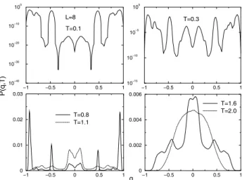
The canonical distribution as a function of the order-parameter is given by:
P(q, T) =
E
G(E, q)e−E/kBT (17)
In Fig. 5, we show a plot of the canonical distribution at different temperatures for one bond configuration of the
L = 8EA model. At low temperatures, there are multi-ple peaks, and the depth of the valleys between peaks de-pends upon temperature. When the temperature is high a single central peak is all that can be seen. At low temper-ature the relative depth of the minima is as great as10−30, and there are several local minima even at higher temper-atures. With conventional Monte Carlo simulations, it is impossible to overcome the barriers at the lower tempera-tures, so the simulation will get trapped in one of the lo-cal minima. Therefore, even two decades after the model was proposed, there are disagreements about the existence of a finite phase transition between a glass phase and a disordered phase. For example, using Monte Carlo sim-ulations on systems as large as (642×128), Marinari et
al. [57] expressed doubt about the existence of the “well-established” finite-temperature phase transition of the 3D Ising spin glass [44, 47]. Their simulational data could be described either by a finite-temperature transition or by an unusualT = 0singularity. Kawashima and Young could also not rule out the possibility ofTg = 0[48]. Thus even
the existence of the finite-temperature phase transition is still controversial, and thus the nature of the spin glass state is uncertain. Although the best available simulational results [13, 52, 58] have been interpreted as a mean-field like behav-ior with replica-symmetry breaking(RSB) [59], Mooreet al.
found evidence for the droplet picture [60] of spin glasses within the Migdal-Kadanoff approximation. They argued that the failure to see droplet model behavior was because all existing Monte Carlo simulations were done at temperatures so close to the transition that system sizes larger than the cor-relation length were not used. It is possible to heat the sys-tem to increase the possibility of escape from local minima by simulated annealing and the more recent simulated tem-pering method [61] and parallel temtem-pering method [62, 63], but it is still very difficult to reach equilibrium at low tem-peratures. Recently Hatano and Gubernatis proposed a bi-variate multicanonical Monte Carlo method for the 3D±J
spin glass model, and their result also favors the droplet pic-ture [16, 64]. Marinariet al. argued, however, that the data were not thermalized [58]. The nature of spin glasses thus remains controversial [51].
5
Summary and Outlook
−1 −0.5 0 0.5 1 0
0.01 0.02 0.03
T=0.8 T=1.1
−1 −0.5 0 0.5 1
10−40
10−30
10−20
10−10
100
P(q,T)
−1 −0.5 0 0.5 1
q
0 0.002 0.004 0.006
T=1.6 T=2.0
−1 −0.5 0 0.5 1
10−15
10−10
10−5
100
T=0.1
T=0.3 L=8
Figure 5. Canonical probability distributions for the 3-dim EA model with one bond distribution.
The application to the Ising model and theq= 10Potts model on square lattices shows that the method is effec-tive for systems that show first order or second-order phase transitions. Although the presentation concentrated on the random walk in energy space the idea is very general and can be applied to any parameters [11]. The energy levels of the models treated here are discrete and the total number of possible energy levels is known before simulation, but in a general model such information is not available. Since the histogram of the random walk with our algorithm tends to be flat, it is very easy to probe all possible energies and monitor the histogram entry at each energy level. For some models where all possible energy levels can not be fitted in the computer memory or the energy is continuous, e.g. the Heisenberg model, a discretization of the energy can be im-plemented.
In this paper, we only applied the Wang-Landau algo-rithm to simple models; but since the algoalgo-rithm is very effi-cient even for large systems it should be very useful in the studies of general, complex systems with rough landscapes. There have already been a significant number of other appli-cations of Wang-Landau sampling including efforts to im-prove sampling [65], to simulate proteins [66] and poly-mer films [67], studies of fluids [68], to study antiferro-magnetic Potts models [69], reaction coordinates [70], for quantum Monte Carlo [71], for the Kondo problem [72], for the study of biological circuits [73], and for combina-torial number theory [74]. Some understanding of the con-vergence and performance limitations of the method have already been provided [75]; however, more investigation is needed to better determine under which circumstances the method offers substantial advantage over other approaches and how the method can be further improved.
Acknowledgments
This research has been supported by the National Sci-ence Foundation under Grant No. DMR-0094422.
References
[1] D. P. Landau and K. Binder,A Guide to Monte Carlo
Meth-ods in Statistical Physics, (Cambridge U. Press, Cambridge, 2000).
[2] N. Metropolis, A. W. Rosenbluth, M. N. Rosenbluth, A. M. Teller and E. Teller, J. Chem. Phys.21, 1087, (1953).
[3] R. H. Swendsen and J.-S. Wang, Phys. Rev. Lett. 58, 86
(1987).
[4] U. Wolff, Phys. Rev. Lett.62, 361 (1989).
[5] B. A. Berg and T. Neuhaus, Phys. Rev. Lett.68, 9 (1992).
[6] B. A. Berg and T. Neuhaus, Phys. Lett. B267, 249 (1991).
[7] W. Janke and S. Kappler, Phys. Rev. Lett.74, 212 (1995).
[8] B. A. Berg and T. Celik, Phys. Rev. Lett.69, 2292 (1992).
[9] N. S. Alves and U. Hansmann, Phys. Rev. Lett. 84, 1836
(2000).
[10] W. Janke, Int. J. Mod. Phys. C3, 375 (1992).
[11] B. A. Berg and U. Hansmann and T. Neuhaus, Phys. Rev. B 47, 497 (1993).
[12] W. Janke, Physica A254, 164 (1998).
[13] B. A. Berg and W. Janke, Phys. Rev. Lett.80, 4771 (1998).
[14] B. A. Berg, Nucl. Phys. B,63, 982 (1998).
[15] B. A. Berg T. Celik and U. Hansmann, Eur. Phys. Lett.22, 63 (1993).
[16] N. Hatano and J. E. Gubernatis inComputer Simulation Stud-ies in Condensed Matter Physics XII, D. P. Landau, S. P. Lewis and H.-B. Schuttler (eds) (Springer, Berlin, Heidel-berg, 2000).
[17] B. A. Berg J. Stat. Phys.82, 323 (1996).
[18] A. M. Ferrenberg and R. H. Swendsen, Phys. Rev. Lett.61, 2635 (1988),63, 1195 (1989).
[19] P. D. Beale, Phys. Rev. Lett.76, 78 (1996).
[20] J. Lee, Phys. Rev. Lett.71, 211 (1993).
[21] P. M. C. de Oliveira, T. J. P. Penna and H. J. Herrmann, Braz. J. Phys.26, 677 (1996).
[22] P. M. C. de Oliveira, T. J. P. Penna and H. J. Herrmann, Eur. Phys. J. B.1, 205 (1998).
[23] P. M. C. de Oliveira, Eur. Phys. J. B.6, 111 (1998).
[24] A. R. Lima, P. M. C. de Oliveira and T. J. P. Penna, J. Stat. Phys.99, 691, (2000).
[25] Jian-Sheng Wang and Lik Wee Lee, Comput. Phys. Commun. 127, 131, (2000).
[26] Jian-Sheng Wang, Comput. Phys. Commun.121, 22 (1999).
[27] B. A. Berg and U. Hansmann, Eur. Phys. J. B6, 395 (1998).
[28] Jian-Sheng Wang, Eur. Phys. J. B.8, 287 (1998).
[29] F. Wang and D. P. Landau, Phys. Rev. Lett.86, 2050 (2001).
[30] F. Wang and D. P. Landau, Phys. Rev. E64, 056101 (2001).
[31] D. P. Landau and F. Wang, Comput. Phys. Commun.147, 674
(2002).
[32] U. Hansmann, Phys. Rev. B56, 6200 (1997).
[33] U. Hansmann and Y. Okamoto, Phys. Rev. E54, 5863 (1996).
[35] F. Y. Wu, Rev. Mod. Phys.54, 235 (1982).
[36] Jian-Sheng Wang, T. K. Tay and R. H. Swendsen, Phys. Rev. Lett.82, 476 (1999).
[37] D. P. Landau, Phys. Rev. B13, 2997 (1976).
[38] A. E. Ferdinand and M. E. Fisher, Phys. Rev.185, 832 (1969).
[39] R. H. Swendsen, J. S. Wang, S. T Li, B. Diggs, C. Genovese and J. B. Kadane, Int. J. Mod. Phys. C,10, 1563 (1999).
[40] K. Binder, K. Vollmayr, H. P. Deutsch, J. D. Reger M. Scheucher and D. P. Landau, Int. J. of Mod. Phys. C5, 1025, (1992).
[41] M. S. S. Challa, D. P. Landau and K. Binder Phys. Rev. B34, 1841, (1986).
[42] K. Binder and A.P. Young, Rev. Mod. Phys.58, 801 (1986).
[43] S.F. Edwards and P.W. Anderson, J Phys. F. Metal Phys.5, 965 (1975).
[44] A.T. Ogielski and I. Morgenstern, Phys. Rev. Lett.54, 928 (1985).
[45] F. Wang, N. Kawashima and M. Suzuki, Europhys. Lett.33,
165 (1996).
[46] F. Wang, N. Kawashima and M. Suzuki, Int. J. Mod. Phys. C. 7, 573 (1996).
[47] R.N. Bhatt and A.P. Young, Phys. Rev. Lett.54, 924 (1985).
[48] N. Kawashima and A.P. Young, Phys. Rev. B53, R484 (1996).
[49] M. Palassini and A. P. Young, Phys. Rev. Lett. 82, 5128
(1999).
[50] M. Palassini and A. P. Young, Phys. Rev. Lett. 83, 5126
(1999).
[51] M. Palassini and A. P. Young, Phys. Rev. Lett. 85, 3017
(2000).
[52] E. Marinari, Phys. Rev. Lett.82, 434 (1999).
[53] M. A. Moore, H. Bokil and B. Drossel, Phys. Rev. Lett.81, 4252 (1999).
[54] J. Houdayer and O. C. Martin, Phys. Rev. Lett. 82, 4934
(1999).
[55] I. Morgenstern and K. Binder, Phys. Rev. B22, 288 (1980).
[56] K. Binder inFundamental problems in statistical mechanics V, edited by E. G. D. Cohen, (North-Holland, 1980).
[57] E. Marinari, G. Parisi and F. Ritort, J. Phys. A27, 2687 (1994).
[58] E. Marinari, G. Parisi, F. Ricci-Tersenghi and F. Zuliani, J. Phys. A34, 383 (2001).
[59] G. Parisi, Phys. Rev. Lett.43, 1754 (1979),50, 1946 (1983).
[60] D. S. Fisher and D. A. Huse, Phys. Rev. B38, 386 (1988).
[61] E. Marinari and G. Parisi, Europhys. Lett.19, 451 (1992).
[62] K. Hukushima and K. Nemoto, J. Phys. Soc. Japan65, 1604
(1996).
[63] K. Hukushima, in Computer Simulation Studies in
Con-densed Matter PhysicsXIII, D. P. Landau, S. P. Lewis and H.-B. Schuttler (eds) (Springer, Berlin, Heidelberg, 2000).
[64] N. Hatano and J. E. Gubernatis, Phys. Rev. B 65, 140513
(2002).
[65] B. J. Schulz, K. Binder, and M. Mueller, Int. J. Mod. Phys. C 13, 477 (2002); C. Yamaguchi and N. Kawashima, Phys. Rev. 65, 0556710 (2002); B. J. Schulz, K. Binder, M. Mueller, and D. P. Landau, Phys. Rev. E67, 067102 (2003).
[66] N. Rathore and J. J. de Pablo, J. Chem. Phys. 116, 7225
(2002); N. Rathore, T. A. Knotts, and J. J. de Pablo, J. Chem. Phys.118, 4285 (2003).
[67] T. S. Jain and J. J. de Pablo, J. Chem. Phys.116, 7238 (2002).
[68] Q. Yan, R. Faller, and J. J. de Pablo, J. Chem Phys.116, 8745 (2002); Q. Yan and J. J. de Pablo, Phys. Rev. Lett.90, 035701 (2003); T. S. Jain and J. J. de Pablo, J. Chem. Phys.118, 4226 (2003); M. S. Shell, P. G. Debenedetti, and A. Z. Pana-giotopoulos, Phys. Rev. E66, 056703 (2002).
[69] C. Yamaguchi and Y. Okabe, J. Phys. A34, 8781 (2001).
[70] F. Calvo, Mol. Phys.100, 3421 (2002).
[71] M. Troyer, S. Wessel, and F. Alet, Phys. Rev. Lett.90, 120201 (2003)
[72] W. Koller, A. Prull, and H. G. Evertz, Phys. Rev. B 67,
104432 (2003)
[73] H.-B. Schttler, et al. (private communication)
[74] V. Mustonen and R. Rajesh (preprint)