Brazilian Journal of Physics, vol. 34, no. 2A, June, 2004 373
Continuous Time Stochastic Models for Vehicular
Traffic on Highways
´
Attila L. Rodrigues and M´ario J. de Oliveira
Instituto de F´ısica, Universidade de S˜ao Paulo, Caixa Postal 66318, 05315-970, S˜ao Paulo, SP, Brazil
Received on 2 September, 2003
We have simulated a continuous time version of the Nagel-Schreckenberger model of vehicular traffic on high-ways and calculated the flux as a function of vehicle density. In the low density regime the flux increases linearly with density but becomes a power law when velocities are allowed to increase without bounds. We have simulated also a modified version in which the state of a vehicle depends on the velocity of the vehicle moving ahead. This model displays a phase transition from a state with nonzero flux to a jammed state at a critical density which is strictly less than the closed-packed density. We also study the relationship of this model with self-organized criticality.
1
Introduction
Vehicular traffic flow is a subject, outside of the traditional areas of physics, that has been the object of investigation by the methods of statistical physics [1-7]. Stochastic nonequi-librium models defined on lattices are useful tools on the study of vehicular traffic from the microcopic point of view [6, 7]. In this approach, the traffic of vehicles is modeled by a system of interacting particles, each particle represent-ing an individual vehicle. The evolution of the system is defined by dynamical irreversible rules implying that these systems should be studied within the framework of nonequi-librium statistical mechanics [8-13]. We will be concerned here with the so called ”particle-hoping” models. Originally, these models were defined as cellular automata, with de-terministic rules, or as probabilistic cellular automata, with stochastic rules. In both cases the updating is synchronous. In this paper, however, we will examine the continuous time version of such models, with sequential updating or, more precisely, random sequential updating and whose time evo-lution of the probability distribution is governed by a master equation.
The stochastic microscopic models which we investigate here are defined by stochastic rules that are suitable for com-puter simulation. Numerical simulations are useful since anlytical approaches for nonequilibrium systems are very difficult to implement. Even though, we will present here some analytical results coming from mean-field approxima-tions and compare them with numerical results. We will fo-cus our attention on a continuous time version of the Nagel-Schreckenberger cellular automata model [14] of vehicular traffic on highways (model A) and a modification of it that takes into account the velocity of the vehicle moving ahead of another one (model B).
The main property we want to find is the relation be-tween the flux and density, usually called the fundamental
diagram of road traffic. For low densities, empiral data [15] shows a linear dependence of the flux on density. Increasing the density, the flux reachs a maximum (maximum capacity) and then drops. These properties are found for both models studied here. For model A, the flux vanishes when the den-sity is the closed-packed denden-sity. However, for model B, the flux vanishes at a critical density which is strictly less than the closed-packed density.
2
Model A
Let us consider a system of N particles moving in a one dimensional lattice withLsites and periodic boudary condi-tions. Each site can be either empty or ocupied by a particle (vehicle). The particles move forwardly and may have any velocity up to a maximum velocity. The position and the ve-locity of thejparticle are denoted byxjandvj, respectively.
The distance between two consecutive sites is a so that
xj =anjwherenj can take the values0,1, ..., L−1. The
velocities of the particles take on discrete valuesvj = uνj
whereνj = 0,1, ..., νm, so that the maximum velocity is
vm=uνm. For simplicity we assumea= 1andu= 1. The state of the system is defined by the collection of the positions{xj}and velocites{vj}of theN particles. The
374 Attila L. Rodrigues and M´ario J. de Oliveira´
then be equal to the number of empty sites between the par-ticle and the one ahead of it. Letjbe the chosen particle and let us denote the new velocity byv′
jand the new position by
x′
j. The rules are then
v′
j= min{ℓj, vj+ 1, vm}, (1) whereℓiis the number of empty sites between the particle
and the one that is moving ahead. The new position is
x′
j =xj+v′j. (2)
We define the interval of timeτ as the time it takes to make N movements of particles or trials (a Monte Carlo step). The time step between two successive movement tri-als will beτ /N. Since there areNparticles the average time between two movements of the same particle will be justτ. Therefore, we must have the following relationu=aτ.
The density of particlesρ =N/(aL)is the number of particle per unit length. Since we are assuminga= 1then
ρ=N/L. The fundamental property we want to analyze is the fluxφof particles as a function of the densityρ. The flux is the average number of particles crossing a certain point per unit time. IfM is the number of particle cross-ing a specified point of the lattice in the time intervalτthen
φ=M/τ. If we denote byvthe average velocity of parti-cles given by
v= 1
N
j
vj. (3)
then the flux is given by
φ=ρv. (4)
0 0.2 0.4 0.6 0.8 1
ρ
0 0.1 0.2 0.3 0.4
φ
1 2 3 4 7 15 inf
Figure 1. Fluxφversus density of vehiclesρfor model A for sev-eral values of the maximum velocityvmobtained from simulation
of system with lattice sizeL= 1000.
−10 −8 −6 −4 −2
ln
ρ
−5 −4 −3 −2 −1
ln
φ
Figure 2. Log-log plot of the fluxφversus density of particlesρ forvm =∞for model A obtained from simulation for a system
with sizeL= 105A straight line fitted to the data points at small densities has slope0.42.
Using rules (1) and (2) we have simulated a system of
N particles with periodic boundary conditions with lattices withLsites. Fig. 1 shows the flux of particles as a function of the density forL = 1000and for several values of the maximum velocityvm. The flux increases linearly at small densities, reaches a maximum and then decreases at high densities. For small densities the flux increases linearly ac-cording to
φ=vmρ, (5) as long asvmis finite. If the maximum velocity is infinite, that is, if the velocity of a particle may increase without bounds, the behavior (5) is no longer valid. We assume then the following power law behavior for small densities
φ∼ρα.
(6) The double-log plot ofφversus ρ, shown in Fig. 2, gives the resultα= 0.42(1). In the high density regime, the flux becomes independent of the maximum velocity. Forρnear
1the flux behaves as
φ= 1−ρ. (7) To set up a mean-field approximation we assume that the stationary state is a non-correlated state. This means that, the probability that there is a gap of sizeℓbetween a given vehicle and the vehicle moving ahead is
Pℓ= (1−ρ)ℓρ. (8)
We assume further that the velocity of the vehicle isvℓ =
min{v, ℓ}. The average velocity will be then
v=
∞
ℓ=0
vℓPℓ=
1−ρ
ρ {1−(1−ρ)
vm}, (9)
which gives the flux
φ=ρv= (1−ρ){1−(1−ρ)vm}. (10)
Brazilian Journal of Physics, vol. 34, no. 2A, June, 2004 375
0 0.2 0.4 0.6 0.8 1
ρ
0 0.2 0.4 0.6 0.8 1
φ
Figure 3. Fluxφversus density of vehiclesρfor model A obtained from a mean-field approximation. The curves correspond, from botton to top, tovm= 1,2,3, and7, respectively.
3
Model B
In this section we set up a model to describe more precisely the interaction between a vehicle, say vehiclei, and the ve-hicle which is moving ahead, veve-hiclei+ 1. In model A the velocity of the former does not depend on the velocity of the latter. In model B, if the velocity of the vehiclei+ 1is zero and the gap between vehiclesiandi+ 1is 1 then the vehicle
iis not alowed to occupy the gap and it remains in its place with zero velocity. Therefore the rules are the same as those given by equations (1) and (2) except whenℓi = 1in which
case the new velocity is given by
v′
j = 0 if vi+1= 0, (11)
v′
j = 1 if vi+1= 0. (12)
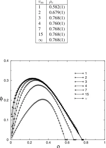
We have simulated model B for several values of the maximum velocity. The flux as a function of the density is shown in Fig. 4. At small densities the behavior is the same as the model A. However, at high density the behavior is entirely distinct from model A. As shown in Fig. 4, there is a critical densityρcabove which the flux vanishes. Table
I shows the values of the critical density for several values of the maximum velosityvm. As one increases the density of vehicles, model B displays, therefore, a nonequilibrium phase transition from a state with nonzero flux to a jammed state with zero flux. The critical behavior of the flux near the transition is
φ∼(ρc−ρ)β, (13)
withβ= 1.
TABLE 1: Critical densityρcfor several values of the
maximum velocity of vehiclesvmfor model B.
vm ρc
1 0.582(1) 2 0.679(1) 3 0.768(1) 4 0.760(1) 7 0.768(1) 15 0.768(1)
∞ 0.768(1)
0 0.2 0.4 0.6 0.8 1
ρ
0 0.1 0.2 0.3 0.4
φ
1 2 3 4 7 15
∨
Figure 4. Fluxφversus density of vehiclesρfor model B for sev-eral values of the maximum velocityvmobtained from simulation
of system with lattice sizeL= 1000.
A jammed configuration is an absorbing state in which all cars have zero velocity. From the time evolution rules we see that any configuration of particles with zero velocity such that the gaps between particles are at most of size one is a jammed state. A jammed configuration may therefore occur whenever half of the sites are occupied so that there are infinitely many absorbing states. We expect then that the phase transition to the jammed state fall within the univer-sality class of systems with infinitely many abosrbing states [16, 17]. Since, the particles are driven to move in a given direction we expect a mean-field behavior and in particular
376 Attila L. Rodrigues and M´ario J. de Oliveira´
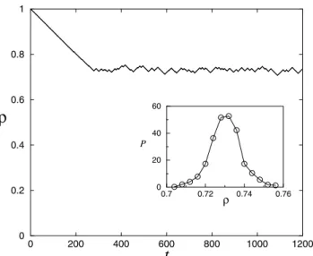
move. If after a certain number of Monte Carlo stepsT, pre-viously defined, the vehicles are still moving, we insert a ve-hicle into the system. If, on the other hand, the flux vanishes, before the maximum timeT, we remove a vehicle, chosen at random. In other words, we remove a vehicle whenever the systems falls into a jammed state and insert one if the flux is nonzero. At the begining the density of vehiclesρin the system decreases linearly from the maximum valueρ = 1
untill it reaches a value where it begins to fluctuates around a certain valueρ∗
of the density as can be seen in Fig. 5 for the case of system sizeL= 1000and maximum number of Monte Carlos stepsT = 1000. The inset of Fig. 5 shows that the density fluctuates around the valueρ∗
= 0.731. The average densityρ∗
depends on the system size L
and on the maximum number of Monte Carlo stepsT, and is expected to approachρcasL→ ∞andT → ∞.
0 200 400 600 800 1000 1200
t
0 0.2 0.4 0.6 0.8 1
ρ
0.7 0.72 0.74 0.76
ρ
0 20 40 60
P
Figure 5. Density of particles for model B with infinity maximum velocity as a function oft, a quantity that increases by one unit whenever a particle is removed or added to the system. The inset shows a histogram of the densities with averageρ∗= 0.731. The
data are taken from a system withL= 1000andT = 1000.
4
Conclusion
We have simulated two stochastic models for vehicular traf-fic on highways. In our approach, the traftraf-fic of vehicles is modeled by a system of interacting particles, each particle representing an individual vehicle. The first model is a con-tinuous time version of the Nagel-Schreckenberger model. In the second we introduce an interaction between a vehicle and the vehicle moving ahead. We found that this second model has a phase transition from a state with nonzero flux to a jammed state which occurs for a density of particles wich is strictly less than the closed-packed density.
Acknowledgements
We wish to thak R. Dickman for helpful comments. We also acknowledge CNPq for finantial support.
References
[1] R. Herman and K. Gardels, Sci. Am.209(6), 35 (1963).
[2] F. A. Haight, Mathematical Theory of Traffic Flow (Aca-demic Press, New York, 1963).
[3] W. D. Ashton,The Theory of Road Traffic Flow(Methuen, London, 1966).
[4] D. C. Gazis, Science157, 273 (1967).
[5] I. Prigogine and R. Herman, Kinetic Theory of Vehicular Traffics(American Elsevier, New York, 1971).
[6] Traffic and Granular Flow (World Scientific, Singapore, 1996), edited by D. E. Wolf, M. Schreckenberg, and A. Bachem.
[7] D. Chowdhury, L. Santen, and A. Schadschneider, Physics Report329, 199 (2000).
[8] T. M. Liggett,Interacting Particle Systems(Spinger-Verlag, New York, 1985).
[9] J. Marro and R. Dickman,Nonequilibrium Phase Transition in Lattice Models(Cambridge University Press, Cambridge, 1999).
[10] T. Tom´e e M. J. de Oliveira,Dinˆamica Estoc´astica e Irre-versibilidade (Editora da Universidade de S˜ao Paulo, S˜ao Paulo, 2001).
[11] B. Schmittmann and R. K. P. Zia, inPhase Transitions and Critical Phenomena(Academic Press, New York, 1995), vol. 17, edited by C. Domb and J. L. Lebowitz.
[12] G. Sch¨utz, in Phase Transitions and Critical Phenomena (Academic Press, New York, 2001), vol. 19, edited by C. Domb and J. L. Lebowitz.
[13] Nonequilibrium Statistical Mechanics in One Dimension (Cambridge University Press, Cambridge, 1997), Edited by V. Privman,
[14] K. Nagel and M. Schreckenberger, J. Physique I 2, 2221 (1992).
[15] F. L. Hall, B. L. Allen, and M. A. Gunter, Transp. Res. A 20, 197 (1986).
[16] R. Dickman, M. A. Mu˜noz, A. Vespignani, and S. Zapperi, Braz. J. Phys.30, 27 (2000).