Sustainability of the U.S. Federal deficit: an updated analysis

(1)

Sustainability of the U.S. Federal Deficit:

an updated analysis.

Dissertação apresentada ao Programa

de Pós-Graduação “Stricto Sensu”

em Economia de Empresas da

Universidade Católica de Brasília,

como requisito para a obtenção do

Título de Mestre em Economia de

Empresas.

Orientador: Professor Doutor

Tito Belchior Silva Moreira

(2)

TERMO DE APROVAÇÃO

Dissertação defendida e aprovada como requisito parcial para obtenção do

grau de mestre no programa de Economia de Empresas, defendida e aprovada,

em de junho de 2007, pela banca examinadora constituída por:

PROF. DR. TITO BELCHIOR SILVA MOREIRA

(Orientador)

PROF. DR. JOSÉ ÂNGELO DIVINO

(Examinador interno)

PROF. DR. GERALDO DA SILVA E SOUZA

(Examinador externo)

(3)

(4)

ACKNOWLEDGMENTS

Many years ago, in Guyana, I visited the home of Mr. Benard Darnel, a

Canadian who was then an economist with the local branch of IDB. Benard was

married to a Brazilian lady and we met quite often. At this particular occasion, I

went to his house to close a deal in my first notebook. On his wall, in a beautiful

frame, there was his Master Diploma, which, I must say, made me long for the

day that I would have a similar one.

Years after, life gave me some lemons, but I turned them into a very

fragrant lemon juice. Among the ingredients of this juice, I place high my

success in achieving the present Master of Sciences in Economics.

Acknowledging everybody who helped me reach this step in my life is a

daunting task. I am afraid to leave people out who, in one way or another, gave

me a hand to be where I am now.

To my parents, for showing the value of learning.

To Francis, for helping me improve my English skills. To Serginho, for

studying with me since the time from Góes and for helping me overcome some

pitfalls found in this dissertation. To Raimundo, for giving me a reality check

when one was in order. To Marçal, for making the call in a time I needed

somebody to call me. To Joni, for sharing the thrills of learning. To all

colleagues who, in one moment or another, gave me a hand and showed me that

I could do it. To all Professors, who believed that an old mule could still learn.

To Professor Tito, who, in his professional way, guided me through such

journey.

(5)

“

L’homme est visiblement fait por penser;

c’est toute sa dignité, et tout son devoir

(6)

This dissertation aims at checking the solvency of the U.S. public debt, using quarterly data ranging from 1947:1 to 2005:4. The long-term equilibrium between receipts and expenditures was evaluated using the Johansen Cointegration Test, and causality and exogeneity test were done to the two series.

The dissertation shows that the debt is solvent; finding that one dollar in expenditures causes receipts to increase in one dollar and forty cents. Moreover, it was found that receipts do not Granger causes expenditures and that expenditures is not weakly exogenous.

(7)

Esta dissertação tem como objetivo principal checar a solvência da dívida pública norte americana com dados trimestrais no período 1947:1 a 2005:4. Avaliou-se o equilíbrio de longo prazo entre receita e despesa com base nos testes de cointegração de Johansen e realizou-se testes de causalidade e exogeneidade.

Conclui-se pela solvência da dívida com relação de um dólar de despesa para um dólar e quarenta para receita. Verificou-se, ademais, que a receita não Granger causa despesa e que a despesa não é fracamente exógena.

(8)

FIGURE 1 – Evolution of U.S. real current deficit, in billions of dollars –

1929-2005……….………12 FIGURE 2 - Real expenditures, inclusive of interest paid on debt, and real receipts –

1947(1) to 2005(2).……..……….26 FIGURE 3 - Evolution of First Differences –Real Expenditures 1947(1) to 2005(2)……….27

(9)

TABLE 5.1: Real receipts & Real Expenditures. ADF results. 1947:1-2005:4………. 29

TABLE 5.2 - Real receipts & Real Expenditures. PP results. 1947:1-2005:4……….30

TABLE 5.3 – Real receipts & Real Expenditures. DF-GLS Modified Akaike test. 1947:1-2005:4………....31

TABLE 5.4 - Real receipts & Real Expenditures. Modified PP results with Spectral GLS-detrended AR based on modified Akaike. 1947:1-2005:4………...……….31

TABLE 5.5 – Johansen Cointegration Test Summary………..34

TABLE 5.6 – Cointegration equation ...………..35

TABLE 5.7 - Vector of Error Correction Estimates………...………..35

TABLE 5.8 – Pairwise Granger Causality Tests on Real Expenditures and Real Receipts – lags 1 to 1....………...……….. 36

(10)

“Economic growth in the United States has been above the historic average and faster than any other major industrialized economy in the world. January was the 41st month of uninterrupted job growth produced by this economy, in an expansion that has thus far added more than 7.4 million new jobs. Unemployment is low, inflation is moderate, and real wages are rising. Our economy is on the move and we can keep it that way by continuing to pursue sound economic policy based on free-market principles.”

However, what this paragraph does not show is the fact that, for quite a few decades,

the American government has been running deficits in order to promote its economy.

Since the times of the New Deal, the American government has been experiencing

with deficit spending in order to pull the economy out of depression, to pay for wars and to

create jobs.

President Roosevelt himself has, in his first year in office, created a budget deficit

almost six times bigger than his predecessor’s last year.

The success of the New Deal, combined with wartime victory and relatively low

employment has shown that government intervention on the economy would give the tone in

spending policy after the Second World War.

For instance, in order to receive back all surviving G.I.s1, the U.S. Congress passed, in

1946, the Full Employment Act, committing the government to pursue low employment

through government intervention in the economy, which included, in several fiscal years,

running a deficit to foot the bill.

The deterioration of public accounts was strong.

1_GI

(12)

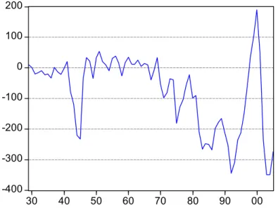
-400 -300 -200 -100 0 100 200

30 40 50 60 70 80 90 00

Figure 1 – Evolution of U.S. real current deficit, in billions of dollars – 1929-2005

As it can be seen on Figure 1, the American government has been facing increasing

amounts of deficit as a result of government incentives to the economy, thus increasing its

Federal public debt. Although the 50’s and 60’s were years of small amounts of surpluses, it

is clear that the American government has let the deficit increase after the first oil shock in

1973. A short period in the 90’s has showed a remarkable return to pragmatism by the

Clinton Administration. However, his efforts were lost after Bush has taken office. Budget

deficits under the Bush Administration increased largely after to the events of September 11

and the subsequent government decision of fighting global terrorism by waging low-level but

costly wars. Moreover, with the aim of keeping employment levels high shows that the U.S.

government has no disposition of changing its policy in the foreseeable future.

1.1 - MOTIVATION

Several studies on the feasibility of such policy have been done. This dissertation aims

at updating such studies with emphasis on the use of several modern econometric methods.

Following datasets already established by different authors, the behavior of Real Receipts and

Real Expenditures from the first quarter of 1947 to the fourth quarter of 2005 is investigated.

A long-term relation using VAR techniques is searched for and the exogeneity of Real

(13)

This dissertation starts with this Introduction. It is followed by a research on the

available literature. Section three shows a simple model for the behavior of the long term

equation found by VAR techniques. The methodology used is found in Section four. Section

five shows all test results. Section six concludes and indicates possible future development on

(14)

2 - LITERATURE REVIEW

A review of the American public debt shows that one can divide the treatment of the

debt by the U.S. government in roughly two eras and two corresponding philosophies2.

According to researched sources, the first era (1861-1932) was dominated by traditional

precepts of public debt management, meaning any budget should be strictly balanced and any

debt arising from war events or any other event should be quickly dealt with. The corollary of

this policy was that the government should meddle the least possible in economic affairs and

that the ups and downs on business cycles were natural phenomena. The government should

try to accumulate budget surpluses only to face times of difficulties.

This era was superseded by what was known as the “New Deal”, the name President

Franklin D. Roosevelt gave to the series of programs between 1933–1937 with the goal of

relief, recovery and reform of the United States economy during the Great Depression. During

this period, the U.S. government experimented with deficit spending in order to pull the

economy out of recession, basically by printing money to fund the works done under the

program. With the start of the Second World War, the American debt soared to a record of

US$ 269,422 million. Notwithstanding, the experience of the New Deal combined with low

unemployment and war victory seemed to confirm Keynesian theories and to reduce the fear

of budget deficits.

After the war, the Congress passed the Full Employment Act, committed to low

unemployment, and with the underlying proposition that the government could run deficits in

order to keep unemployment levels low. Despite massive foreign aid, the sharp recession in

the late ‘50s and the Korean War, presidents Truman and Eisenhower were traditionalists at

heart and they managed to present budget surpluses more than half of their respective fiscal

years.

From 1960 to 1975, this view of public spending changed drastically. During this

period, governments in place could run only one fiscal year of budget surplus. With the

Kennedy administration, Keynesianism reached its heights as de-facto policy within

government:

“In the 1960s and 1970s, tax cuts and increased domestic spending were pursued not only to improve society but also to move economy toward full employment. However, these economic stimulants were not just applied on down cycles of the economy but also on up cycles, resulting in ever-growing deficits.” (Noll, not dated).

2

(15)

The Vietnam War had worsened the down effects of such policy and, by 1975, the

United States was suffering from stagflation and budgetary deficits seemed to be out of

control. Despite this picture, the passing of the Budget Control Act, which had its effects felt

at the start of the fiscal year 1975, worsened this picture. Previously, the impoundment

authority of the President gave him the ability to refrain from spending funds authorized in

the budget. For instance, the President could in effect veto a project included in the Budget by

the Congress by not releasing funds through the Treasury. The Act changed the balance of

power between the Executive and Legislative branches in favor of the latter and public debt

soared in the decades following the enactment of the Act.

In view of the above, the fact that U.S. government could embark on running annual

deficits forever has interested many a research. Simply put, the research focused not anymore

on the ability of the government to pay the debt in total, but whether the government would be

able to run this fiscal policy indefinitely. According to Quintos (2005):

“A government that operates in a dynamically efficient economy balances its budget intertemporally by setting the current market value of debt equal to the discounted sum of expected future surpluses. A violation of intertemporal budget balance would indicate that the fiscal policy cannot be sustained forever because the value of debt would explode over time at a rate faster that the growth rate of the economy. Thus a sustainable fiscal policy is one that would cause the discounted value of debt to go to 0 at the limit so that the present-value borrowing constraint would hold.”

Quintos brings thus into attention the view of running an economy in a dynamic way,

by which the actions of government take into consideration not only present but future times.

According to Martin (2000), authors who run tests on the U.S. deficit sustainability

roughly followed two paths: Hamilton and Flavin (1986) and Wilcox (1989) concentrated

their analysis on the univariate properties of debt, whereas Trehan and Walsh (1988), Hakkio

and Rush (1991)3, Haug (1991), Tanner and Liu (1994) and Quintos (1995) verified the

cointegration properties of government revenue and expenditure, with some analysts

incorporating structural breaks.

In reviewing some of these authors, it was found that Hamilton & Flavin (1986)

showed in a seminal article that the federal government cannot run a permanent deficit

exclusive of interest payments on the debt, but may have a constant deficit when interest

payments are included. Their key result is that the real rate of interest at which the

government borrows must be greater that the growth rate of real debt so that the discounted

present value of future government debt goes to zero. Furthermore, they shown that the

surplus (or deficit) inclusive of debt payments should be stationary in order for the

3

(16)

government budget to be balanced in present value terms. They present their claim by

analyzing data from 1960 to 1984 and found that the reviewed U.S. data backed the assertion

that the government budget historically has been balanced in expected present-value terms.

In an article which was cited but not read, Kremers (1988) demonstrates that this result

is not robust to lag specification in the test.

Wilcox (1989) took a different view of Hamilton & Flavin. His work extends

Hamilton & Flavin findings in three aspects: First, it allowed for stochastic real interest rates,

whereas the former authors assumed a fixed real interest rate. Second, it allowed for

nonstationarity in the noninterest surplus, whereas Hamilton & Flavin required the surplus to

be stationary. Third, Wilcox’s paper had power against stochastic violations of the borrowing

constraint, whereas two of the tests of Hamilton & Flavin assumed that any violation of the

borrowing constraint would be nonstochastic. Applying new tests, Wilcox found that the

period 1960-1084 could not be treated as a whole, for he found strong evidence of shifts in the

structure of fiscal policy. According to the author, for the period prior to 1974, the borrowing

constraint was satisfied, and the structure of fiscal policy of running debts could have been

maintained forever. However, for the period after 1974, this constraint seemed not to be

satisfied. His paper, thus, contrasts its findings with those of Hamilton & Flavin as he states

that the fiscal policy in implementation after 1974 was not sustainable.4

Trehan and Walsh (1991) extend previous works, which used cointegration, in two

directions. First, they relaxed the requirements that expenditures and revenues to be difference

stationary, while maintaining the assumption of a constant expected real rate of interest, and

showed that the cointegration test continues to be valid as long as a quasi difference of the

net-of-interest deficit is stationary. According to the authors, if the interest-inclusive deficit is

stationary, intertemporal budget balance holds, and this measure of the deficit is the

appropriate error correction term. Second, they examined what happens if the expected rate of

interest is not a constant. They showed that the cointegration test is generally no longer valid.

They proved that, as long as the expected real rate of interest is positive, intertemporal budget

balance holds if the inclusive-of-interest deficit is stationary. They examined data on the

federal government’s budget and found that a stationary linear combination of the stock of

debt and the net-of-interest deficit did not exist. However, as said, the first difference of the

stock of debt is stationary. They interpreted this finding to imply that the deficit process is

consistent with sustainability, but that the assumption of constant expected real rate was a bad

4

(17)

approximation to the data. Second, they checked whether foreigners were holding an

unsustainable large amount of U.S. debt and found that the data could reject this hypothesis.

Bohn (1995) reexamines the theoretical foundations of the sustainability question by

studying government policies in an explicitly stochastic general equilibrium model, in which

individuals may be risk averse. His main message was that the (then) existing empirical tests

were based on too simple and inappropriate theoretical models.

The author cites various empirical studies (Hamilton & Flavin (1986), Hakkio & Rush

(1989), Kremers (1989), Trehan & Walsh (1988, 1991), Wilcox (1989) and Roberds (1991)).

According to Bohn, zero limit on the on the expected value of future debt is not correct (as

Hamilton and Flavin and Wilcox have found) but it can diverge to infinity. Therefore a zero

limit is not a necessary condition for sustainability in a stochastic economy.

Quintos (1995) looked for structural changes in the rank of the cointegration matrix

instead of looking for changes in cointegrating vector parameters. The former searches for

long term changes in the very relationship, whereas the latter searches for changes in the

parameters which characterize the long term relationship. The author showed increase in gap

between series mid-70’s onward. She used Phillips and Ploberger (1994) posterior

information criterion (PIC) and ADF tests. For the real tax revenue series, results favor unit

root with PIC= 19.25, l = 1, p= -1 (i.e., no intercept) and the coefficient on the first lag being

1.005. ADF was equal to -0.11, which falls below the 5% critical value and favors the

unit-root hypothesis. Real expenditure series show PIC= 3.069e-05, l= 2, and p= -1, with the

coefficient on the first lag in levels being 1.0097. PIC value clearly does not favor a unit-root

model, and a coefficient of 1.0097 suggests an explosive root. ADF was -.40, which indicates

that a test for a unit root should be done against an alternative of an explosive root. Her

conclusions on whether fiscal US fiscal policy was consistent with intertemporal budget

balance and whether there has been a structural change in deficit policy was that there was a

shift in deficit policy in the early 80’s. In other words, revenues and expenditures inclusive of

interest paid had cointegrating vector (1, -1) for the pre-break period, but they are not

cointegrated in the post-break period with 0<b<1. The finding of a break in the deficit process

in more uncertain when variables are normalized by GNP and population. Regardless of

whether or not there is a shift in policy she showed that the deficit was sustainable.

Ghosh (1995) exploits the close analogy between a consumer trying to smooth

consumption and a government trying to minimize tax distortions in order to test a very tight

set of restrictions on the joint time series process for budget deficits, government revenues,

(18)

strategy on the optimal path of the tax budget rather on tax rates themselves. He explains that

the assumption of tax smoothing implies that the budget surplus should equal the expected

present discount value of the change in government expenditure. The prediction that the

budget surplus should equal the present discounted valued of expected changes in government

expenditure allowed Ghosh to construct a time series for the optimal budget surplus (SURt*)

and to compare it to the actual surplus (SURt). Under the null hypothesis that the government

seeks to smooth taxes these two series should differ at most by sampling error. An additional

implication is that the budget surplus should Granger-cause changes in government

expenditure (Gt, equal to expenditures minus interest payment on debt). Ghosh found that unit

Root Tests on Gt cannot reject the null of nonstationarity. The null of a unit root in SURt

could be rejected for the United States. Additionally, SURt was found to granger-causes

changes in Gt, so the data is consistent with the most basic implications of the tax-smoothing

behavior. SURt and SURt* (model) are highly correlated: + 0.96 for the USA. The

intertemporal tax-smoothing model is remarkably successful in explaining the behavior of the

US federal government budget deficit.

Crowder (1997) tests the stability of the U.S. federal intertemporal budget constraint

over the postwar period using a new recursive test conducted within the framework of the

maximum likelihood estimator. The implied equilibrium budget path is estimated and used to

determine which component of the budget has greater responsibility for the recent

intertemporal violations. Using data from 1950(1) to 1994(2), Crowder concludes that there is

a violation of the long-run equilibrium between real expenditures and real revenues of the

U.S. Federal Debt and that this violation is created by the rise on real expenditures. His results

are reinforced by an analysis of the revenues/GDP and expenditure/GDP ratios. According to

his data, the change in the deterministic trend in the expenditures/GDP series explains all of

the divergence of trends in the two ratios. Moreover, Crowder found that the federal

government appeared to have been obeying its intertemporal budget constraint until 1982, a

date which conformed well to his a priori belief that the deficit “exploded” in the early part of

the Reagan administration.

In our current century,

(19)

In view of the above, Martin (2000) re-examined the sustainability issue using a new

approach, based on the cointegration model for U.S. government revenue and interest

inclusive expenditure, with allowance made for multiple endogenous breaks in both the

intercept and slope parameters. According to the author, this

“Methodology produces simultaneous inferences about the presence of cointegration, the value of the cointegrating parameters and the size and timing of shifts in the relationship. Thus, inference about cointegration is not conditional on pre-imposed breakpoints, or is inference about the breakpoints conditional on the presence of cointegration. Rather, a potentially cointegrating relationship, with possible deterministic shifts, is estimated over the whole sample period and one set of results derived.”

Using quarterly data from 1947(2) to 1992(3), the author found evidence of

cointegration between revenue and interest inclusive expenditure, as well as evidence to

suggest that the pre-shift coefficient on expenditure is unity. As such, strong sustainability of

the deficit process, prior to any shift, is indicated. He also found that shifts on both the

intercept and slope of the deficit process are estimated as occurring in 1975(1), 1985(1), and

1987(1) and that the most substantial shifts occurred in the intercept term, effecting a

proportionately large net decrease in the level of regression. The slope shifts, also according

to the author, are small and almost offsetting, suggesting little change in the initial value close

to unity and thereby implying maintenance of strong sustainability over the full period.

Instead of using classical approaches based on I(1) or I(0) integration techniques

Cunado et al (2002) examined if sustainability of the US fiscal deficit holds using a

methodology based on fractional processes. They used fractional process because, recently, it

has become a rival class of alternatives to the AR model in case of unit-root tests.

Specifically, their study updated previous studies (Hakkio and Rush and Quintos) and

their results showed that U.S. real revenues and government expenditure are both integrated

of order 1 variables. However, looking at the differences between both variables, they found

mixed results. According to them,

“If the underlying disturbances are white noise, the unit root null hypothesis cannot be rejected, implying that there is no cointegration vector (1, -1). From an economic point of view, this result suggests that the U.S. fiscal deficit is not sustainable.”

This conclusion was in line with Hakkio and Rush and Quintos, who found evidence

of sustainability only for a sub-sample ending in 1980. Notwithstanding, the order of

(20)

fractional cointegration existed between both variables. Their results showed that the public

deficit in the U.S. is therefore an I (d) process with d slightly smaller than 1, implying that

fiscal deficit is mean reverting, and thus, sustainable, though the adjustment process towards

equilibrium would take a very long time.

Bajo-Rubio et al (2006) re-examined the long-run sustainability of US budget deficits,

using Bai and Perron´s multiple structural change approach. Their procedure allows to test

endogenously for the presence of multiple structural changes in a estimated relationship, and

has a number of advantages over previous approaches: the underlying assumptions are less

restrictive, confidence intervals for the break dates can be calculated, the data and errors are

allowed to follow different distributions across segments, and the sequential method used in

the application can allow for the presence of serial correlation in the errors and heterogeneous

variances across segments. Moreover, as in this dissertation, the period of analysis extends to

2005, including the most recent developments in the evolution of the U.S. budget deficit.

The authors found a cointegration between federal government revenues and

expenditures, inclusive of interest paid on debt, with 0 <

^

β< 1, meaning the U.S. fiscal deficit would have been only weakly sustainable over the full sample 1947:1 – 2005:3, therefore

confirming, for a more extended period, what Quintos and Martin had previously found. A

flaw of this study is that the author used data for the U.S. government as a whole, instead of

using data for the Federal government only. This flaw masks out payments made between

U.S. state and federal levels and are therefore roughly inflated.

However, their main objective was the use of a multiple endogenous break model,

applying Bai and Perron (1998, 2003) methodology. According to the results, they have found

breaks at 1955:3, 1982:1, and 1996:3, thus providing four sub-samples. The first and second

regimes (1947:1-1955-2 and 1955:3-1981:4) showed that the U.S. budget deficit would have

been only weakly sustainable as in the whole sample. In the third regime (1982:1-1996:2) the

U.S. budget deficit would have been strongly sustainable. However, in the fourth regime

(1996:3-2005-3), no long-run relationship between public revenues and expenditures would

appear.

Finally, Payne and Mohammadi (2006) addressed the possible nonlinear effects of

fiscal policy actions and examined the long-run sustainability of the U.S. budget deficit after

(21)

budgetary process? 2) Is the sustainability of budget deficits robust to structural breaks and/or

shifts in fiscal policy regimes? and 3) are there asymmetries in the response of the budget

deficit to deviations from its long-run trend?

Not only did Payne and Mohammadi updated past studies but they also reexamined

the “strong form” of budget deficit sustainability5, thus extending previous research by testing

for the possibility of asymmetries in the response of the budget deficit to deviations from its

long-run trend. They used seasonally adjusted data for the period 1947:1 to 2003:4 for the

ratio of federal government budget deficit to GDP, and they found that the budget deficit

underwent a dramatic shift in 1982:1 through 2004:4. Allowing for the existence of structural

break, their results supported stationary and sustainable budget deficits. The follow-up of such

conclusion was that the sustainability of the budget deficit is not robust to structural and fiscal

policy regime shifts. They have also found that the budget deficit adjusts symmetrically

around the threshold value.

5

(22)

3 - THE MODEL

Following Hakkio and Rush (1991), cited in Quintos (1995), the dynamic budget

constraint is as following. The government’s one-period budget constraint is given by

t r t

t G R

B = −

∆ , (1)

Where Bt is the market value of federal debt, Gtr = Gt + rtBt-1 is government expenditure

inclusive of interest payment, and Rt represents tax revenues. All variables are in real terms.

As rt is assumed to be stationary around the mean r and (1) can be written as

t t t

t r B E R

B −(1+ ) ₋₁ = − , (2)

Where Et = Gt + (rt – r)Bt-1 is Gtr with interest rates taken around a zero mean. Because (2) holds for

every period, substituting forward will yield

∑

∞ = + + ∞ → + + + ₋ ₊ = 0 1 1 lim ) ( j j t j j j t j t j

t R E B

B γ γ , (3)

Where = (1+r)-1. Taking (3) and making the difference of Bt (e.g. ∆ Bt) is written as

∑

∞ = + + ∞ → + + − _∆ ₋_∆ ₊ _∆ = − 0 1

1₍ ₎ _lim

j j t j j j t j t j t r

t R R E B

G γ γ , (4)

Where (4) is derived by applying the difference operator ∆ in (3) and using (1).

For (3) or (4) to impose a constraint similar to the intertemporal budget constraint faced by an

individual, it must hold that

0 lim_→_∞ +1∆ t+j =

j

t B

E γ (5)

In (4) [or lim_→_∞ +1 t+j =0

j

t B

E γ in (3)]. If (5) is satisfied, then intertemporal budget balance or deficit

sustainability holds because this would require that the government run future surplus equal, in

expected present-value terms, to its current market value of debt.

(23)

“To test Condition (5), the procedure in the literature is to test for the stationarity of ∆Bt, or

alternatively to test for the stationarity of Gtr – Rt [ if both series are each I (1)] with cointegration

vector (1,-1) imposed. An equivalent procedure is to test of cointegration in the regression equation

t r t

t bG

R =µ + +ε (6)

And to test b=1.”

Quintos, in her research, have found b to be in the interval 0 < ≤ 1 and argues that this

condition is a necessary and sufficient condition for deficit sustainability and that cointegration is only

a sufficient condition.

Finding to be smaller than unity will represent a risk to the ability of governments to market

its debt in the long run. Defining the regression form of the form found on (6) above, it can be shown

that6:

1. The deficit is “strongly sustainable” if and only if I (1) processes Rt and Gt are cointegrated

and = 1.

2. The deficit is only “weakly sustainable” if Rt and Gt are cointegrated and 0 < < 1.7

3. The deficit is unsustainable if ≤ 0.

Therefore, as informed, the purpose of this dissertation is to demonstrate if condition “one”

holds for the entire period under study for both Real Receipts and Real Expenditures.

6

As in Martin (2000).

7

(24)

4 -METHODOLOGY

As to track closely previous studies on the same subject (see Quintos (1995), Martin (2000)

and Cunado et al (2004)), the following series were used from the Bureau of Economic Analysis:

1. Federal Government Current Receipts [Billions of dollars]; Seasonally adjusted at annual

rates;

2. Federal Government Current Expenditures inclusive of debt payment [Billions of dollars];

Seasonally adjusted at annual rates; and

3. Implicit Price Deflators for Gross Domestic Product [Index numbers, 2000=100] also

seasonally adjusted.

The use of such series is standard in the literature. However, only few studies have advanced

the study of such series beyond the end of last century. As explained, this dissertation aims at updating

such analysis with the most current data.

According to the U.S. Bureau of Economic Analysis:

“Seasonal adjustments remove recurring seasonal variations (variations that occur in the same month or quarter each year) from economic series so that the remaining movements in the series better reflect cyclical patterns in economic activity.”

Another advantage of using such series lays on the fact that unadjusted series would

require the use of season dummies to write off the effect of such variations, thus creating

more disturbances on their econometric analysis.

Data used ranged from the first quarter of 1947 to the last quarter of 2005. The use of

such period is due to the fact that, prior to 1947, the U.S. government provided only annual

data.

Interest payments included were shown net of interest receipts, thus reflecting the

actual interest paid on debt.

(25)

Unit Root tests, Cointegration Analysis using Johansen Cointegration Test, Causality

(26)

5 -TEST RESULTS

I followed Quintos (1995) in the construction of the data set. However, I extended the

period used by this author (1947-1992) up to the 4th quarter of 2005, therefore including both

the Clinton administration (1993-2001) and the Bush administration up to the most available

date at the time of research (2002 to 2005).

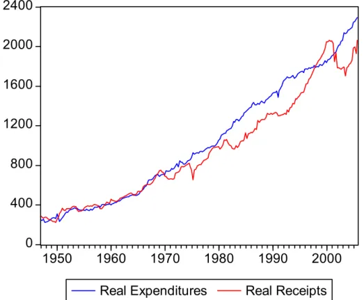
Figure 2 plots the real revenues and real expenditures series for the period. As Quintos

has shown, there is a significant gap between the series from the mid-70s until the beginning

of the Clinton administration. Real receipts have increased significantly during the 90´s and

surpassed real expenditures at the end of the decade. However, there is a sharp drop in

revenues at current century and deficit has resurfaced.

0 400 800 1200 1600 2000 2400

1950 1960 1970 1980 1990 2000

Real Expenditures Real Receipts

Figure 2 - Real expenditures, inclusive of interest paid on debt, and real receipts – 1947(1) to 2005(2)

(27)

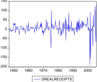
The graph of Real Expenditures, on first difference, shows a mean around zero, which

indirectly might imply a stochastic trend. The same occurs for Real Receipts, on first

difference.

-80 -60 -40 -20 0 20 40 60 80

1950 1960 1970 1980 1990 2000

DREALEXPENDITURES

Figure3 - Evolution of First Differences –Real Expenditures 1947(1) to 2005(2)

-200 -150 -100 -50 0 50 100 150

1950 1960 1970 1980 1990 2000 DREALRECEIPTS

(28)

Both graphs give the impression that real expenditures and real receipts are I (1)

processes.

A visual inspection of correlograms for the two series showed them to be

non-stationary. For real expenditures, even at lags up to 36, the autocorrelation function never dies

out and the estimated autocorrelations, ρs, fall only slightly from 0,987 (lag 1) to 0,570 (lag

36), an indication of a high degree of correlation of this series with its past values. The

analysis for real receipts showed the same pattern. If we include all observations, this series

showed correlation up to lag 73.8

5.1 -UNIT ROOT TESTS

To test the stationarity of both series, several criteria were used. Among them, the

ADF criterion was used, for:

“The simple Dickey-Fuller unit root test … is valid only if the series is an AR(1) process. If the series is correlated at higher order lags, the assumption of white noise disturbances is violated. The Augmented Dickey-Fuller (ADF) test constructs a parametric correction for higher-order correlation by assuming that the series follows an AR(p) process.”9

Although both series seem to represent an AR(1) process, the ADF test includes any

AR(p) process and was therefore used in this study.

Heij et al. (2004, 597) informs

“one should make sure not to exclude the trend term if the series has a clear direction, as otherwise the alternative hypothesis of the (unit root) test corresponds to a stationary time series, so that the test has little chance of rejecting the null hypothesis of a stochastic trend.”

Moreover, Hamilton (1994, 501) suggests to include, for series such as those used in

this thesis, an estimated regression of the type

t t

t y t

y =α +ρ ₋₁+δ +µ (1)

8

See appendix for correlogram graphics.

9

(29)

thus including both a constant and a trend.10

In view of the above, ADF tests with a constant; and a constant and a linear trend were

run.

For the standard ADF test, the choice of lag length was made using Campbell and

Perron (1991) top-down criterion. They explain:

“Start with some upper bound on k, say kmax, chosen a priori. Estimate an

Autoregression of order kmax. If the last included lag is significant (using the standard normal asymptotic distribution), select k=kmax. If not reduce the order of the estimated Autoregression by one until the coefficient on the last included lag is significant. If none are significant, select k=0.”

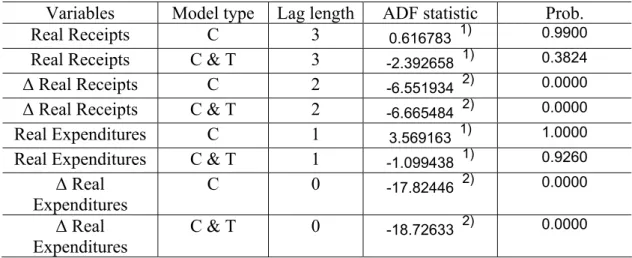
Unit Root tests using Campbell and Perron’s lag criteria are shown below:

Table 5.1: Real receipts & Real Expenditures. ADF results. 1947:1-2005:4 Source: Own elaboration.

- C means constant only

- C & T means constant & trend

- ∆ represents first difference of the series under study - ADF statistics are not in absolute values

- 1) Series under study is non-stationary - 2) Series under study is stationary

10

According to Marques, in “Teste de Cointegração para a paridade do poder de compra para o Brasil – evidências do efeito Balassa-Samuelson”, when explaining the Johansen test, the utilization of a trend and a intercept for cointegration equations... provides more generalization to long-run relations.” As the Johasen test is a multivariate generalization of the Dickey-Fuller test for unit root, it seems plausible to include both trend in intercept in both ADF and Johansen tests.

Variables Model type Lag length ADF statistic Prob.

Real Receipts C 3 0.616783 1) 0.9900

Real Receipts C & T 3 -2.392658 1) 0.3824

∆ Real Receipts C 2 -6.551934 2) 0.0000

∆ Real Receipts C & T 2 -6.665484 2) 0.0000

Real Expenditures C 1 3.569163 1) 1.0000

Real Expenditures C & T 1 -1.099438 1) 0.9260

∆ Real Expenditures

C 0 -17.82446 2) 0.0000

∆ Real Expenditures

(30)

As the series in analysis have both a clear upward direction, the relevant test equation

is of the type of shown in (1), where the error terms µ_t should be a normally distributed white noise. However, as Heij et al. (2004, 598) put

“time series are often characterized by short-term fluctuations in the sense that the detrended series is correlated over time. The above model neglects this, so that the residuals will be serially correlated and the critical values will not be valid. For the Dickey-Fuller t-test, we can apply a Newey-West correction for serial correlation to compute the standard error of the estimated parameter ρ. … If this correction is applied, the Dickey-Fuller critical values remain valid asymptotically. The t-test based on the Newey-West standard error of ρ is called the Phillips-Perron test.”

As both series have the characteristics shown above, the Phillips-Perron test was also

applied to them, with the following results:

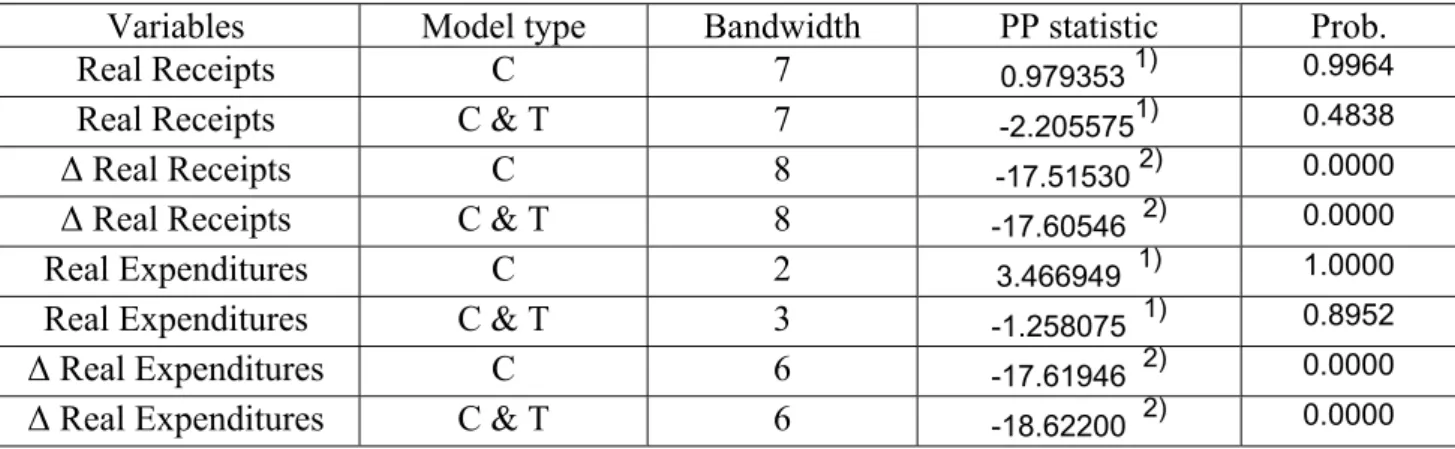
Variables Model type Bandwidth PP statistic Prob.

Real Receipts C 7 0.979353 1) 0.9964

Real Receipts C & T 7 -2.2055751) 0.4838

∆ Real Receipts C 8 -17.51530 2) 0.0000

∆ Real Receipts C & T 8 -17.60546 2) 0.0000

Real Expenditures C 2 3.466949 1) 1.0000

Real Expenditures C & T 3 -1.258075 1) 0.8952

∆ Real Expenditures C 6 -17.61946 2) 0.0000

∆ Real Expenditures C & T 6 -18.62200 2) 0.0000

Table 5.2 - Real receipts & Real Expenditures. PP results. 1947:1-2005:4 Source: own elaboration

- C means constant only

- C & T means constant & trend

- ∆ represents first difference of the series under study - 1) Series under study is non-stationary

- 2) Series under study is stationary - Automatic Bandwidth selection.

Such traditional tests receive criticism in the literature for showing sample size

distortions and/or low potency. Therefore, modified ADF and Philips-Perron tests were used,

following Elliot, Rottemberg and Stock (1986) and Ng and Perron (2001). Both tests confirm

(31)

ADF test showed that the first difference of Real Expenditures to be non-stationary. This

particular result was dismissed as all other tests showed this first difference to be stationary.

Variables Model type Lag Length MADFGLS

Real Receipts C 3 2.218493 1)

∆ Real Receipts C 10 -2.679211 2)

Real Expenditures C 12 2.233672 1)

∆ Real Expenditures C 11 -0.768506 1)

Table 5.3 – Real receipts & Real Expenditures. DF-GLS Modified Akaike test. 1947:1-2005:4

Source: Own elaboration. - C means constant only

- 2) Series under study is stationary

Variables Model type Lag Length Adj. t-Stat

Real Receipts C 3 0.642653 1)

∆ Real Receipts C 4 -25.16064 2)

Real Expenditures C 12 1.234195 1)

∆ Real Expenditures C 11 -81.14969 2)

Table 5.4 - Real receipts & Real Expenditures. Modified PP results with Spectral GLS-detrended AR based on modified Akaike. 1947:1-2005:4

Source: Own elaboration. - C means constant only

- 2) Series under study is stationary

As with most economic series, real expenditures and real receipts were confirmed to

(32)

5.2 - JOHANSEN COINTEGRATION TEST

The difference between American real receipts and real expenditures should be stable

over time in order to the American government debt to be payable. Notwithstanding, a

structural approach revealing the relationship between these two variables may be flawed by

the wrong specification of the dynamics of such relationship. Furthermore, estimation and

inference may be marred by the fact that endogenous variables can be found on both sides of

the equations.

Heij et al. (2004, 656) explain the dangers of neglecting the endogeneity of

explanatory variables with the following example:

“Suppose that the variables yt and xt are generated by the model

t t

t y

y =φ ₋₁+η , x_t =γy_t₋₁+ω_t

Assuming that 0 < Ø < 1 and γ ≠0and η_t and ω_tare independent white noises. yt is an

AR(1) process that is independent of xt, and xt depends on the past of yt. …Suppose that we

(wrongly) assume that xt is exogenous in the regression model y_t =βx_t +ε_t… if the

endogeneity of xt is neglected, then this regression gives the wrong impression that the

variable xt would affect the variable yt.”

In such cases, a vector autoregressive (VAR) model of order 1, which is a direct

generalization of the univariate AR(1) model to the case of a vector of variables, is to be used.

As the variables used in this study are both AR (1) we may thus use a VAR modeling to

predict the long-run relationship between them.

5.3 - THE CHOICE OF LAG STRUCTURE

Issler & Lima (2000), on a study on the sustainability of the Brazilian public debt,

warn us that

“The results of co-integration tests using this technique (Johansen’s technique) depend on the deterministic components included in the VAR and on the chosen lag length.”

The choice of lag length is thus crucial in VAR specification for its results show high

sensitivity if the model is improperly specified. Too little lags can generate distortions on the

size of tests, whereas too many lags may cause loss of power for these tests.

Therefore, a pre-test was made using all criteria provided by the software package

(33)

VAR specification. Results of testing the lag length criteria for a VAR estimated with an

unrestricted constant term varied according to the chosen criteria. For instance, LR, Akaike’s

information criterion (AIC) and Final Prediction Error (FPE) criteria showed the model to be

more adequate when including 4 lags. Hannan-Quinn information criterion suggested the use

of three lags. Finally, Schwarz information criterion (also called the Bayes information

criterion – BIC) suggested a model with only one lag.

When reviewing an extensive evaluation of which lag length selection criteria one has

to employ (Liew (2004)), it was found that AIC and FPE should be a better choice for smaller

samples. With relatively large samples (120 or more observations), Hannan-Quinn criterion is

found to outdo the rest in correctly identifying the true lag length. The data sample for this

dissertation amounted to 236 observations. Using Liew’s suggestion only, one would choose a

length of three lags for this dissertation. However, the author also states that all criteria

“Are designed in such a way that larger lag length is less preferable, in the spirit of parsimony (that is the simpler the better).”

With the Johansen Co-integration Test, co-integration was not possible after the

inclusion of two lags for, when including three or more lags, the summary of trend

assumptions showed that, under most data trend specifications, there were 2 co-integrations

equations, which could represent a sign of misspecification for a model with only two

variables or the fact that the variables under study were stationary, and they are not.

Even when running the only Johansen Cointegration Test which showed only one

cointegration relation under both trace and Max-eingenvalue tests (Data trend: linear, with 1

to 3 lag interval), the coefficients for the cointegrating equation were found not to be

significant.11

Therefore, in the spirit of the statistical preference for the most parsimonious model,

the third best fit was chosen, with a lag structure of one to one lag interval.12

With this decision taken, assumptions were made about trends. A summary of all 5

trend assumptions was generated in order to determine the choice of trend assumption. The

only two trend assumption which provided only one cointegration relation for both the Trace

11

Their values divided by their respective standard errors were found not to be under the value of 2.

12

(34)

and Max –Eigenvalue test were type 2 (no intercept and no trend in the CE) and type 4

(intercept and trend in the CE)

In her book “The Cointegrated VAR Model: Methodology and Applications (Advanced Texts in Econometrics)”13, Katarina Juselius explains that

“Given linear trends in the data, case 4 is generally the best specification to start with unless we have strong beliefs that the linear trends cancel in the cointegration relations.”

A Johansen Cointegrating Test, type 4 with a 1 to 1 lag interval structure was run.

Unfortunately, the coefficients of the correspondent cointegrating equation were not

significant, for their division by their respective t values were not above 2. This result was

consistent with those found when unit root tests were performed, as they showed that the null

of unit root was accepted using constant or using constant and tendency.

As the only remaining data trend structure with two cointegrating relations was type 2

structure a new test was run with a 1 to 1 lag interval. The results for this test are shown

below.

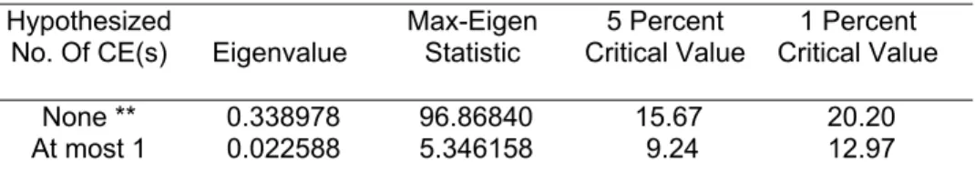
Unrestricted Cointegration Rank Test

Hypothesized Trace 5 Percent 1 Percent

No. Of CE(s) Eigenvalue Statistic Critical Value Critical Value

None ** 0.338978 102.2146 19.96 24.60

At most 1 0.022588 5.346158 9.24 12.97

*(**) denotes rejection of the hypothesis at the 5%(1%) level

Trace test indicates 1 cointegrating equation(s) at both 5% and 1% levels

Hypothesized Max-Eigen 5 Percent 1 Percent

No. Of CE(s) Eigenvalue Statistic Critical Value Critical Value

None ** 0.338978 96.86840 15.67 20.20

At most 1 0.022588 5.346158 9.24 12.97

*(**) denotes rejection of the hypothesis at the 5%(1%) level

Max-eigenvalue test indicates 1 cointegrating equation(s) at both 5% and 1% levels

Table 5.5 – Johansen Cointegration Test Summary Intercept (no trend) in CE – No intercept in VAR Lag interval – 1 to 1

In this case, all coefficients were found to be significant at 5%.

13

(35)

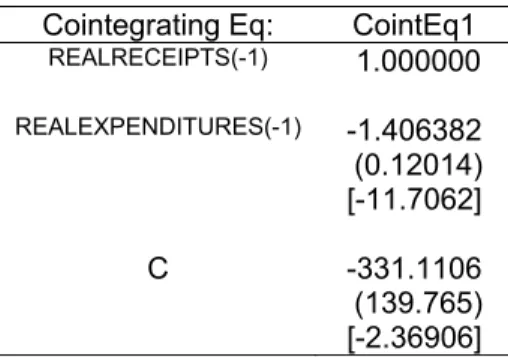
The Cointegration equation and the Vector Error Corrections Estimates for the same

deterministic trend specification are given below:

Cointegrating Eq: CointEq1

REALRECEIPTS(-1) _1.000000

REALEXPENDITURES(-1) _-1.406382

(0.12014)

[-11.7062]

C -331.1106

(139.765)

[-2.36906]

Table 5.6 – Cointegration equation

Error Correction: D(REALREC EIPTS)

D(REALEXP ENDITURES)

CointEq1 -0.012955 -0.012833

(0.00262) (0.00141)

[-4.94847] [-9.12288]

D(REALRECEIPT S(-1))

-0.180245 -0.042601

(0.06615) (0.03554)

[-2.72478] [-1.19858]

D(REALEXPENDI TURES(-1))

-0.157191 -0.215876

(0.12144) (0.06525)

[-1.29443] [-3.30850]

Table 5.7 - Vector of Error Correction Estimates

Parameters of this VEC were significant, except for some parameters related to some

of the differences of the series under study. However, the F statistics are relatively high, thus

we cannot reject the hypothesis that, collectively, all lagged terms are statistically significant.

Table 5.6 provided the following Cointegrating equation:

(36)

The equation shows that, for every dollar spent in expenditures, the US government is

able to raise roughly US$ 1.40 in receipts. This is a demonstration that, for the period under

analysis, the US debt is solvent.

Full Estimates for the Vector of Error Correction are found in Annex C.

5.4 - CAUSALITY TEST

According to the Keynesian Effective Demand principle, as government expenditures

increase so does national income. As government revenues are mainly derived from taxation

on national income, one can assume that an increase on government expenditures will cause

an increase on government revenues. However, empirical evidence on the causality between

U.S. Real Receipts and Real Expenditures at the federal level are mixed. Anderson et al.

(1986) found causality of expenditures to revenues. Blackley (1986) and Manage and Marlow

(1986), apud Park (1998), found that revenue increases led to spending increases.

In view of these mixed findings a causality test is in order when a VAR procedure is

used for Real Receipts and Real Expenditures, for, throughout this thesis, it was assumed that

an increase on Real Expenditures would cause a rise on Real Receipts, thus validating the

Keynesian principle.

In this context, one should verify whether Expenditures are in fact an exogenous

variable. Firstly, in order to verify weak exogeneity, a causality relation is to be found

between Receipts and Expenditures.

A Granger causality test was thus performed on the series under study, as these series

fulfilled the requirements for such tests: both series are non stationary but they cointegrate.

Granger causality tests are sensitive to lag selection. One should set the lag selection

on the VAR and use the same for Granger causality tests. With the previously-used lag

selection (1 to 1), we found that that Real Receipts does not Granger cause Real Expenditures

(probability above 0.05) and Real Expenditures does Granger cause Real Receipts

(probability under 0.05).

Null Hypothesis: Obs F-Statistic Probability

REALEXPENDITURES does not Granger Cause REALRECEIPTS

235 9.59794 0.00219

REALRECEIPTS does not Granger Cause REALEXPENDITURES

0.06943 0.79241

(37)

5.5 -EXOGENEITY TEST

Causality tests should be used in conjunction with exogeneity tests. The importance of

checking whether a variable is weakly exogenous (or strongly exogenous) derives from the

fact that, when one assumes that a variable is exogenous in a model, it can in fact be an

endogenous variable. In uniequation models, when one assumes that a variable is exogenous

when it is not, the equation can be improved by a system of equations.

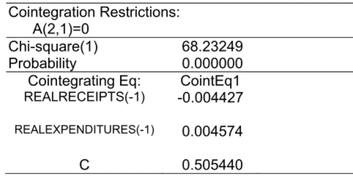
Following Johansen’s procedure (1992) to check for exogeneity (apud Eviews, 544), the null of Real Expenditures to be weakly exogenous in the above-mentioned VEC was

rejected.

Cointegration Restrictions: A(2,1)=0

Chi-square(1) 68.23249

Probability 0.000000

Cointegrating Eq: CointEq1

REALRECEIPTS(-1) -0.004427

REALEXPENDITURES(-1) _0.004574

C 0.505440

(38)

6 -CONCLUSIONS

This dissertation found that, in spite of the rapid deterioration of U.S. public accounts

at the end of last century, in the long run the American government can still claim that their

fiscal deficit is sustainable.

Although both series under study were found to be not stationary, a stable long run

relationship between them, using Johansen’s procedure, could be established.

The value of found in this dissertation ( =1.4) shows that the U.S. federal debt is

actually strongly sustainable. These findings are not so out of place with recent studies, for

Bajo-Rubio et al., for instance, when considering a more recent sub-period, found a much higher value ( = 4.3).

The dissertation also showed that conditions for weak exogeneity were not found for

Real Expenditures. Notwithstanding, this lack of finding should no invalidate the assumption

that an increase in real expenditures by the U.S. government may increase in the long run its

receipts.

The data also showed that the efforts of Clinton’s administration to produce surpluses

were wasted away since President Bush came into power. Although present deficits can be

justified by the current fight on global terrorism, even a rich nation as the United States has to

come to grips with the harsh reality of balancing the budget in the long run.

A suggestion for further work would be waiting for the Bush Administration to end

and see how the U.S. federal deficit behaved under both Presidents Clinton and Bush as a

sub-period. Although contemporary American History has shown that a Democrat president

normally supersedes a Republican one, there is no guarantee against the possibility that an

equal free-spending president will replace Mr. Bush and will further worsen the U.S. federal

(39)

REFERENCES

1. ARAUJO, ELIANE CRISTINA DE AND DIAS, JOILSON. “Endogeneity of financial sector and economic growth: an empirical analysis of the Brazilian

economy.” Rev. econ. contemp., Sept./Dec. 2006, vol.10, no.3, p.575-609. ISSN 1415-9848.

2. BAJO-RUBIO, O., DÍAZ-ROLDÁN, C. AND ESTEVE, V.: "US deficit sustainability revisited: a multiple structural change approach", Working Paper 19/05, Instituto de Estudios Fiscales. New version: May 2006. Forthcoming in Applied Economics.

3. BOHN, HENNING, 1995. "The Sustainability of Budget Deficits in a Stochastic Economy," Journal of Money, Credit and Banking, Ohio State University Press, vol. 27(1), pages 257-71, February.

4. Bureau of Economic Analysis (BEA) – Methodology Papers: U.S. National Income and Product Accounts. September, 2005.

5. ________________________________ - National Income and Product Accounts Table (NIPA tables) downloadable at http://www.bea.gov/national/nipaweb.

6. CAMPBELL, JOHN Y. AND PERRON, PIERRE, 1991. “Pitfall and Opportunities: What macroeconomists should know about unit roots”. NBER Working Papers Series, Technical Working Paper No. 100.

7. CROWDER, WILLIAM J., 1997. "The U.S. Intertemporal Budget Constraint: Restoring Equilibrium Through Increased Revenues or Decreased Spending?" Macroeconomics 9702002, EconWPA, revised 17 Feb 1997.

8. CUNADO, JUNCAL, GIL-ALANA, LUIS A. AND GRACIA, FERNANDO PÉREZ

DE, 2002. "Is the US Fiscal Deficit Sustainable? A Fractionally Integrated and Cointegrated Approach," Faculty Working Papers 03/02, School of Economics and Business Administration, University of Navarra. Published, Journal of Economics and Business, 2004, vol. 56(6): pp. 501-526.

9. DICKEY, DAVID .A. AND FULLER, WAYNE A., 1979. “Distribution of the

Estimators for Autoregressive Time Series with a Unit Root,” Journal of the American Statistical Association, 74, 427–431.

10.ENGLE, R. F., HENDRY, D. F., RICHARD, J. F., 1983. “Exogeneity”.

Econometrica, v. 51, p. 277-304. 11.EVIEWS help book, version 4.1.

(40)

13.GHOSH, ATISH R, 1995. "Intertemporal Tax-Smoothing and the Government Budget Surplus: Canada and the United States," Journal of Money, Credit and Banking, Ohio State University Press, vol. 27(4), pages 1033-45, November.

14.GUJARATI, DAMODAR N., Basic Econometrics. São Paulo: Makron Books, 2000.

15.HAMILTON, JAMES D. Time Series Analysis. New Jersey: Princeton University Press, 1994.

16.HAMILTON, JAMES D. AND MARJORIE FLAVIN, 1986. "On the Limitations of Government Borrowing: A Framework for Empirical Testing", American Economic Review, Vol. 76, No. 4, September 1986. PP. 808-819.

17.HEIJ, CHRISTIAAN; PAUL DE BOER; PHILIP H. FRANSES; TEUN KLOEK;

HERMAN K. VAN DIJK. Econometric Methods with Applications in Business and Economics. New York: Oxford University Press Inc., 2004.

18.HENDRY, DAVID F., JUSELIUS, KATARINA. "Explaining Cointegration Analysis: Parts I and II," Discussion Papers 00-20, University of Copenhagen. Department of Economics (formerly Institute of Economics).

19.HSIAO CHIYING & CHEN PU, 2004. "Testing Weak Exogeneity in Cointegrated System," Econometric Society 2004 Far Eastern Meetings 537, Econometric Society.

20.ISSLER, JOÃO V. & LIMA, LUIZ R., 2000. “Public Debt Sustainability and Endogenous Seigniorage in Brazil: Time Series Evidence from 1947-92”, Journal of Development Economics, vol. 62, no. 1, pp. 131-147.

21.JHA, RAGHBENDRA AND SHARMA, ANURAG, 2001. "Structural Breaks and Unit Roots: A Further Test of the Sustainability of the Indian Fiscal Deficit" ANU Working Paper. Available at SSRN: http://ssrn.com/abstract=280334 or DOI: 10.2139/ssrn.280334. Downloaded in 05/31/2007.

22.JOHANSEN, SØREN. “The interpretation of cointegrating coefficients in the cointegrated vector autoregressive model”, Preprint No. 14. Department of Theoretical Statistics – University of Copenhagen. 2002.

23.__________________ “Cointegration: overview and development”. Available in www.math.ku.dk/~sjo . Downloaded in 06/10/2007. Forthcoming 2007 in Handbook of Financial Econometrics. Springer.

24.JUSELIUS, KATARINA- “The Cointegrated VAR Model: Methodology and

Applications (Advanced Texts in Econometrics)”.Oxford University Press, USA; 2 edition.

(41)

26. MARTIN, GAEL M., 2000. "US deficit sustainability: a new approach based on multiple endogenous breaks," Journal of Applied Econometrics, John Wiley & Sons, Ltd., vol. 15(1), pages 83-105.

27.NG, SERENA & PERRON, PIERRE, 2001. "Lag Length Selection and the Construction of Unit Root Tests with Good Size and Power," Econometrica, Econometric Society, vol. 69(6), pages 1519-1554, November.

28.NOLL, FRANKLIN - The United States Public Debt, 1861 to 1975. Downloaded in 09/21/2006 from http://eh.net/encyclopedia/article/noll.publicdebt .

29.PARK, W. K, 1998. “Granger Causality between Government Revenues and Expenditures in Korea”, Journal of Economic Development, vol. 23(1), June.

30.PARKE, WILLIAM R., 1999. "What Is Fractional Integration?," The Review of Economics and Statistics, MIT Press, vol. 81(4), pages 632-638, November.

31.PAYNE, JAMES & MOHAMMADI, HASSAN, 2006. "Are Adjustments in the U.S. Budget Deficit Asymmetric? Another Look at Sustainability," Atlantic Economic Journal, International Atlantic Economic Society, vol. 34(1), pages 15-22, March.

32.PHILLIPS, PETER C.B. & PERRON, PIERRE, 1986. "Testing for a Unit Root in Time Series Regression," Biometrika, 30. 75, 2. 335-346.

33.QUINTOS, CARMELA E, 1995."Sustainability of the Deficit Process with Structural Shifts," Journal of Business & Economic Statistics, American Statistical Association, vol. 13(4), pages 409-17, October.

34.REIMAN, MARK A., HILL, CARTER R., HILL, CARTER, R., GRIFFITHS,

WILLIAM E. AND JUDGE, GEORGE, G. Using EViews for Undergraduate Econometrics. New Jersey: John Wiley & Sons, Inc. 2001. 2ed.

35.SACHSIDA, A. “Teste de Exogeneidade sobre a correlação poupança doméstica e investimento.” Texto para Discussão No. 659, Instituto de Pesquisa Econômica Aplicada (IPEA), julho de 1999, ISSN 1415-4765.

36.TREHAN, BHARAT & WALSH, CARL E, 1991. "Testing Intertemporal Budget Constraints: Theory and Applications to U.S. Federal Budget and Current Account Deficits," Journal of Money, Credit and Banking, Ohio State University Press, vol. 23(2), pages 206-23, May.

(42)

APPENDIX A

Real expenditures correlogram - 36 lags.

Date: 12/04/06 Time: 16:03 Sample: 1947:1 2005:4 Included observations: 236

Autocorrelation

Partial

Correlation AC PAC

.|******** .|******** 1 0.986653 0.986653

.|*******| .|. | 2 0.973354 -0.00491

.|*******| .|. | 3 0.960259 0.000989

.|*******| .|. | 4 0.946773 -0.02142

.|*******| .|. | 5 0.933798 0.012366

.|*******| .|. | 6 0.920847 -0.00598

.|*******| .|. | 7 0.907967 -0.00356

.|*******| .|. | 8 0.894896 -0.01449

.|*******| .|. | 9 0.882215 0.008182

.|*******| .|. | 10 0.869568 -0.00556

.|*******| .|. | 11 0.856387 -0.02639

.|****** | .|. | 12 0.844131 0.027124

.|****** | .|. | 13 0.832171 0.004765

.|****** | .|. | 14 0.820164 -0.00715

.|****** | .|. | 15 0.807615 -0.02854

.|****** | .|. | 16 0.795546 0.011905

.|****** | .|. | 17 0.784084 0.01655

.|****** | .|. | 18 0.772799 0.001595

.|****** | .|. | 19 0.761803 0.002503

.|****** | .|. | 20 0.750841 -0.00413

.|****** | .|. | 21 0.739971 -0.00124

.|****** | .|. | 22 0.729307 0.000512

.|****** | .|. | 23 0.718573 -0.00845

.|***** | .|. | 24 0.708177 0.00751

.|***** | .|. | 25 0.697259 -0.02444

.|***** | .|. | 26 0.686741 0.007131

.|***** | .|. | 27 0.676289 -0.00441

.|***** | .|. | 28 0.665679 -0.00918

.|***** | .|. | 29 0.65474 -0.01903

.|***** | .|. | 30 0.643795 -0.0062

.|***** | .|. | 31 0.632616 -0.01623

.|***** | .|. | 32 0.621454 -0.00486

.|***** | .|. | 33 0.609858 -0.02358

.|***** | .|. | 34 0.598296 -0.00523

.|**** | .|. | 35 0.586649 -0.00903

.|**** | .|. | 36 0.574918 -0.01138

(43)

APPENDIX B

Real receipts correlogram - 36 lags. Date: 12/04/06 Time: 16:07

Sample: 1947:1 2005:4 Included observations: 236

Autocorrelation

Partial

Correlation AC PAC

.|******** .|******** 1 0.986 0.986

.|*******| .|* | 2 0.974 0.078

.|*******| *|. | 3 0.96 -0.074

.|*******| .|. | 4 0.945 -0.03

.|*******| .|. | 5 0.933 0.054

.|*******| .|. | 6 0.92 0.008

.|*******| .|. | 7 0.908 -0.011

.|*******| .|. | 8 0.895 0.002

.|*******| .|. | 9 0.883 -0.008

.|*******| .|. | 10 0.872 0.044

.|*******| .|. | 11 0.86 -0.056

.|*******| .|. | 12 0.847 -0.025

.|****** | .|. | 13 0.835 0.03

.|****** | .|. | 14 0.823 0.006

.|****** | .|. | 15 0.812 -0.004

.|****** | .|. | 16 0.801 0.018

.|****** | *|. | 17 0.787 -0.105

.|****** | .|. | 18 0.775 0.033

.|****** | *|. | 19 0.76 -0.103

.|****** | .|. | 20 0.744 -0.042

.|****** | .|. | 21 0.728 -0.02

.|***** | .|. | 22 0.712 -0.005

.|***** | .|. | 23 0.696 -0.02

.|***** | .|. | 24 0.679 -0.019

.|***** | .|. | 25 0.664 0.027

.|***** | .|. | 26 0.649 0.008

.|***** | .|. | 27 0.635 0.003

.|***** | .|. | 28 0.62 -0.03

.|***** | .|. | 29 0.605 -0.006

.|***** | .|. | 30 0.591 0.008

.|**** | .|. | 31 0.576 -0.005

.|**** | .|. | 32 0.562 -0.005

.|**** | .|. | 33 0.549 0.014

.|**** | .|. | 34 0.535 -0.002

.|**** | .|. | 35 0.522 0.019

.|**** | .|. | 36 0.51 0.007

It is worth mentioning that, for a total number of 236 observations, the confidence interval of 95% include up to 74 observations, and thus we cannot reject the hypothesis that the real ρk is zero, e.g., that there is no correlation between lags. This is further evidence that

Sustainability of the U.S. Federal deficit: an updated analysis