Estimation of Horizontal Diffusivity on East Coast of Peninsular India

Estimation of Horizontal Diffusivity on

East Coast of Peninsular India

N.Ashok kumar1, V.Arutchelvan2, P.Chandramohan3 1

Assistant Professor, 2 Professor, Department of Civil Engineering, Annamalai University

1

[email protected], [email protected] 3

Director, Indomer Coastal Hydraulics, Chennai

Abstract—Dye diffusion study to obtain the horizontal diffusivity is often carried now a day. Data obtained by Indomer coastal hydraulics by conducting dye tracing experiments at several parts of coastal India, were used and have been analyzed to estimate horizontal mixing coefficients. The data of these studies are used to find out the dispersion coefficients and the oceanic diffusivity is reviewed. Analysis of the data from the 3 sites which had the most complete data sets showed that the horizontal dispersion coefficient ranged from 0·443×106to 6.5×106cm2/sec. The estimated mixing coefficients are compared with those values obtained by earlier studies

Keyword-Dye, Rhoda mine-B, Diffusion, Horizontal mixing coefficient, Coastal Waters

I. INTRODUCTION

Two methods are employed generally to obtain the horizontal diffusivity of the coastal waters. In one method turbulent velocity component of the current meter data is analysed to obtain the horizontal diffusivity. The other method uses the dye diffusion study. In fairly calm regions of the sea without prominent divergence or convergence, the horizontal diffusion is likely to be dominant and the dye diffusion study supposedly gives a good estimate of horizontal diffusivity. Such dispersion studies were more or less limited to the open ocean so far [1] reported the eddy diffusion coefficients ky and kz to have the values of 3.06 x 108cm2/sec and 0.054 cm2/sec respectively for the Equatorial Indian Ocean.

Rhoda mine dyes are generally preferred to other chemicals and radioisotopes for the estimation of diffusivity in the sea, because of (a) the remarkable detectability of the rhodamine family of dyes, especially Rhoda mine B—concentrations smaller than 0.03 µg/kg may be detected in a modern fluorometer, and (b) the simplicity of fluoro metric testing procedures— special training is not required and dye concentrations are determined instantaneously without special preparation of the sample. Further Rhoda mine (B) is considered most accessible, stable, harmless and convenient to use for environmental investigations [2]. Rhoda mine dye tracing is used by government and municipal agencies, national research laboratories, universities, and industrial groups in several applications, which include stream flow measurements, estuarine dispersion studies, herbicide tracing, and ground-water studies.

The number of methods for estimating the magnitude of horizontal diffusion coefficient was summarized [3]. Using the available data on dye diffusion along the east coast of India, the horizontal diffusivities of coastal waters are estimated. The overall characteristics of horizontal diffusivity in this coastal region are reviewed.

II RHODAMINE DYE EXPERIMENT

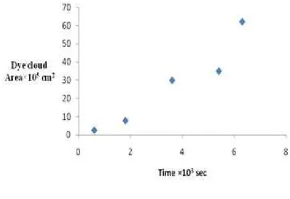
small boat and the barrel opened on both ends at the point of injection. In this experiment, the dye concentration in the vertical direction is assumed to be homogeneous and it is traced continuously using in-situ flurometer. The time taken to trace the dye concentration over the whole diffusing patch increases as the patch grows. During the final stage of the growth, the patch breaks up into several smaller patches. An alternative method of dye cloud observation is to take aerial photographs, which give only its area. The area of the dye cloud increases with time attains a maximum and finally vanishes from the sea surface. During the 100 hours or so of the experiments the area of the dye patches grew from less than 1 km2 to more than 50 km2 [4].

The motion of the patch of the diffusing dye patch in the sea is a sort of irregular meandering of its centre of mass, and we are interested mainly in the distribution of the diffusing substance around the centre of mass. At a time t after the release, the shape of the isolines of dye concentration will be always irregular in an individual experiment and the point of maximum concentration may not necessarily coincide with the centre of mass, while it is reasonable to expect the relative distribution around the respective centres of mass to have the same statistical properties, since eddies with sizes less than or equal to that of the diffusing patch determine the distribution of concentration in the patch. The irregularity in the shape of isolines is caused by the local shear in ocean currents transporting the dye patch and the non-homogeneity of the larger scale turbulence in the sea. Measured horizontal concentration distributions constructed as lines of equal concentration are shown in Figs. A and b. It is clear that the dye patches show a tendency to elongate in the direction of the mean current with a clockwise curvature from the leading edge to the trailing edge. The leading edge of the elongated dye patch generally contained higher dye concentrations than the trailing edge .These features of dye patch diffusion are no doubt attributed to wind-induced Ekman transport and the associated vertical current shear in the mean flow. Similar observations have been made by others. The horizontal dye distribution usually appears asymmetrical in the sense that the characteristic length is larger in one direction the other.

Hence, dye releasing experiments are supposed to be carried out for a large number of times with the same amount of dye solution. When we super impose an infinite number of such dye distributions observed at the same time interval after the beginning of each experiment upon each other, in such a way that the centers of mass coincide, and when we average over all the superimposed distributions, we can expect a rotationally symmetric distribution of substance (owing to a premise that the smaller eddies responsible for the relative distribution are stationary and homogeneous and even isotropic) around the centre of mass; which in other words, the concentration distribution in the mean picture of the diffusing dye patch due to turbulence is only a function of time’t’ and distance ‘r’ from the centre of mass.

seen that the average concentration distribution of the dye is a measure of the probability density function of the marked particle being found at a distance r from the centre of mass after time t. With this approach a diffusion equation is derived (Okubo, 1962), which gives the space-time distribution of the concentration of diffusing substance in the sea as,













−

=

m

m n

t

k

m

r

n

kt

M

C

exp

)

(

where C is dye concentration, M is the value related to the total dye quantity, r is the radius from centre of mass of the patch, t is time and k, m and n are parameters of the diffusion theory adopted.

The parameters and some important values related to different diffusion theory were given by [5]. The lifetime for dye cloud, T, and the time the dye cloud attains the maximum tm.

III. ESTIMATION OF DIFFUSION PARAMETER.

From the measured maximum concentration at the centre of the patch, the apparent horizontal diffusion coefficient could easily be computed. However, as it cannot be guaranteed that the maximum concentration really occurs at the centre of the patch, this method might give relatively higher value for the coefficient. For example, the plume centre line may not be steady, resulting in a meandering plume (see Kristensen, Jensen & Petersen 1981 for example). Additionally, the dispersion coefficient may not be constant, but instead may vary with location, or even with the plume characteristics itself [6].

Fig. 1 Dye cloud area Vs Time.

By fitting the measured distributions of dye release experiments to the theoretical space-time distribution (Eqn. 1) the diffusion parameter k corresponding to different theories can be determined.

1 i i 1 i i i

t

t

S

S

k

−

−

=

The equivalent radius ri associated with the dye cloud area is given by,

π

−

=

2

S

S

r

The other technique to obtain horizontal diffusivity is to regard the peripheral concentration of a dye cloud as constant and the equivalent dye cloud radius r with respect to time t is fitted to the reduced form of Eqn. (1)[7] given by,

(

)

(

)

(

)

t

t

e

r

t

mk

t

t

r

r

_log

log

2

1

−

=

Fig. 2 Fitting of dye cloud area with oceanic diffusion theories.

Based on the method originally proposed by [8] for the atmospheric diffusion, which is applicable for the simple Fickian diffusion law, a generalized method to include various theories of oceanic diffusion is proposed. In this method, the concentric horizontal dye distribution given by Eq. (1) is assumed. Assuming the peripheral concentration discernible by an aerial photograph is constant, the dispersion radius of the dye concentration distribution is defined as, Because of t

)

5

....(

2

/

2





=

r

C

r

dr

C

r

dr

r

π

π

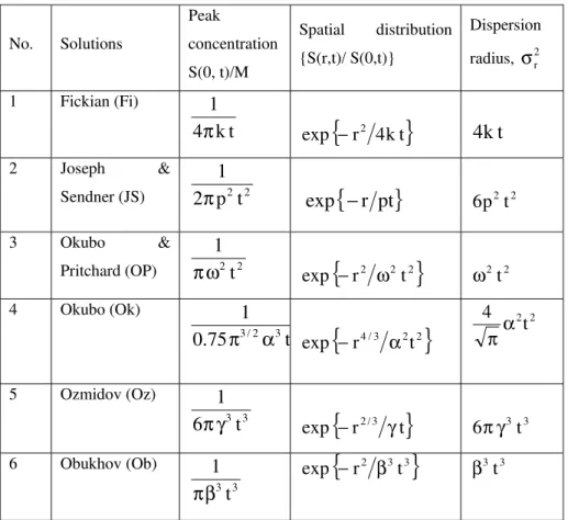
The dispersion radii for various theories of oceanic diffusion are given in Table 1. Eliminating time dependence from the solution of the diffusion equation (1) using the result of Eq. (5), and noting that the radius r vanishes at the lifetime T, one obtains the expression for dispersion radius,

σ

σ

[

]

r m

/ 2 2 m 2

2

r

a

r

ln

(

b

r

e

)

ln

−

σ

−

=

σ

where constants a and b are given in Table 2. Fig. 5 gives the relationship between dye dispersion and dye cloud radius as given by Eq. (6) for two typical cases of Okubo-Pritchard (OP) and Obukov (Ob) (two cases give the identical relationship), and Ozmidov (Oz). It shows that the dispersion radius uniformly increases as the dye cloud radius increases, hits the maximum and then decreases to null. Fig gives the typical application of this method by plotting the dispersion radius calculated from Eq. (6) out of the data of Fig. 2 versus time.

Comparing with the time dependence of the dispersion radius given in Table 1, the theory of either OP or Ob appears to have an edge over that of Ob. Okubo [6] used data from 20 carefully selected instantaneous dye release experiments,

with time scales ranging from 2 hr to 1 month, and length scales ranging from 30 m to100 km. He assumed that the dye experiments were radially symmetric, thus computed the variance for a radially symmetric distribution (σrc2).

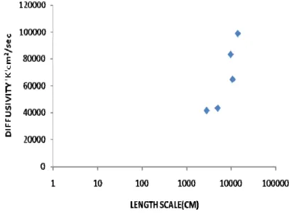
Fig .3 Horizontal diffusivity calculated with the simple method Eq. (2). At various coastal seas

Table 1 Important features of different solutions

IVCONCLUSION

To calculate the dispersion radius out of the dye cloud radius is an excellent method since in that the time dependency of the dispersion radius is simple and straightforward. From the available data the simple method applied to obtain the horizontal diffusivity versus the length scale as shown in Figure.3, and it should be regarded as the basic data for the coastal, calm sea. One can draw a conclusion and pleases to apply any of the oceanic diffusion theory given in Table.1.Horizontal mixing and dispersion in the region is strongly influenced by the prevailing wind.

Dispersion coefficients are found to be the order of 0·443×106to 6.5×106cm2/sec which is the order of magnitude higher compared to the coefficients used for the modelling of surf zone by [9] and also the work done by [10] but they are Clear and logical with the values measured by [11] in similar oceanographic conditions. At the initial stages of diffusion, when the dye patch is small (order of hundreds of meters), marked anisotropy of turbulence, combined with 'shear diffusion' due to vertical shear in the horizontal mean current, gives rise to an apparent increase in the longitudinal diffusion of the patch, whereas for large diffusion times, when the patch increase to the size of kilometres, localized, non-uniformities in the flow do not appear to influence the overall diffusion of the patch.

No. Solutions Peak concentration S(0, t)/M Spatial distribution {S(r,t)/ S(0,t)} Dispersion radius,

σ

1 Fickian (Fi)

t

k

4

1

π

exp

{

−

r

4

k

t

}

4

k

t

2 Joseph & Sendner (JS)

2

p

t

1

π

exp

{

−

r

pt

}

t

p

6

3 Okubo & Pritchard (OP) 2 2

t

1

ω

π

{

}

t

r

exp

−

ω

t

ω

4 Okubo (Ok)

3 2 / 3

t

75

.

0

1

α

π

{

}

t

r

exp

−

α

2 2

t

4

α

π

5 Ozmidov (Oz)

3 3

t

6

1

γ

π

exp

{

−

r

γ

t

}

t

6

π

γ

6 Obukhov (Ob)

3 3

t

1

β

π

{

}

t

r

exp

−

β

The value of effective eddy diffusivity reported by [12] as 24.7 x 106cm2/sec and 1.2 x 106 cm2/sec for Visakhapatnam during March and December (1991) respectively showing a higher value of eddy diffusion by one order under rough weather conditions.

ACKNOWLEDGMENT

I would to like thank Dr. P.Chandra Mohan., Director, Indomer Coastal Hydraulics, Chennai for providing the data obtained by them and also thank Dr.R.Mahadevan., Associate Director, Indomer Coastal Hydraulics for his assistance in the preparation of this manuscript.

REFERENCES

[1] Bahulayan, N. and Varadachari, V.V.R., Determination of vertical velocities in the equatorial part of the Western Indian Ocean Ind.J Mar Sci., 14,2, 55-58., 1985.

[2] Pritchard, D.W. and Carpenter, J.H.,1960 'Measurements of Turbulent Diffusion in Estuarine and Inshore waters', Hydrological Sciences Journal, 5: 4, 37 — 50 Online publication date: 29 December 2009.

[3] Yanagi,T Coastal Oceanography Terra scientific Publishing company,Tokyo,161pp,1999.

[4] Sundermeyer, M. A., and J. R. Ledwell Lateral dispersion over the continental shelf: Analysis of dye-release experiments, J. Geophys. Res., 106(C5), 9603– 9622, 2001.

[5] Okubo, A. Horizontal diffusion from an instantaneous point-source due to oceanic turbulence, Johns Hopkins University Technical Report p32,1962.

[6] Okubo,A Oceanic Diffusion Diagrams, Deep sea research 1971 vol 18 pp789 to 802,1971.

[7] Adachi, S., Nakamura, S. and Mori, A. Experimental study on advection and diffusion in a bay, Proceedings of the 21st Conference of Coastal Engineering, 303-308, 1974.

[8] Gifford F., Relative atmospheric diffusion of Smoke Puffs, Journal of Meteorology, Vol. 14, p.410,1957.

[9] Rodriguez, A.Sanchez. Arcilla,A. Redondo,J.M., Bhahia,E. and sierra J.P,Pollutants dispersion in the nearshore region; Modelling and measurement. Water. Science. Technoplgy. Vol. 32, No. 9-10, pp. 169-175, 1995.

[10] Takewaka.S., Misaki.S., and Nakamura.T, Dye diffusion Experiment in a long shore current field, Coastal Engineering Journal, Vol.45 no.3 pp471-487,2003.

[11] Johnson, D. and Pattiaratchi, C. Transient rip currents and near shore circulation on a swell dominated beach Journal of geophysical research vol.109, 2004.