Annales Geophysicae (2003) 21: 1897–1910 cEuropean Geosciences Union 2003
Annales
Geophysicae
Barometric tides from ECMWF operational analyses
R. D. Ray1and R. M. Ponte2
1NASA Goddard Space Flight Center, Greenbelt, Maryland, USA
2Atmospheric and Environmental Research, Inc., Lexington, Massachusetts, USA
Received: 18 October 2002 – Revised: 23 March 2003 – Accepted: 25 March 2003
Abstract. The solar diurnal and semidiurnal tidal oscilla-tions in surface pressure are extracted from the operational analysis product of the European Centre for Medium Range Weather Forecasting (ECMWF). For the semidiurnal tide this involves a special temporal interpolation, following Van den Dool et al. (1997). The resulting tides are compared with a “ground truth” tide data set, a compilation of well-determined tide estimates deduced from many long time series of station barometer measurements. These compar-isons show that the ECMWF (analysis) tides are significantly more accurate than the tides deduced from two other widely available reanalysis products. Spectral analysis of ECMWF pressure series shows that the tides consist of sharp central peaks with modulating sidelines at integer multiples of 1 cy-cle/year, superimposed on a broad cusp of stochastic energy. The integrated energy in the cusp dominates that of the side-lines. This complicates the development of a simple empir-ical model that can characterize the full temporal variability of the tides.
Key words. Meteorology and atmospheric dynamics (waves and tides)
1 Introduction
The spectrum of atmospheric surface pressure exhibits strong peaks at diurnal and semidiurnal periods, a well-known man-ifestation of the solar atmospheric tides. These global at-mospheric oscillations, forced primarily by water-vapor and ozone radiational absorption, constitute a major part of the total surface pressure variance in the tropics and make an im-portant contribution to the local daily cycle elsewhere. The tides have long been studied both in their own right (Chap-man and Lindzen, 1970) and for what they potentially re-veal about the atmosphere (e.g. Wilkes, 1949; Cooper, 1982; Hamilton, 1983; Braswell and Lindzen, 1998). Our work is partly motivated by modern oceanographic and geodetic ap-Correspondence to:R. D. Ray ([email protected])
plications: tidal pressure waves load the ocean and land, and the resulting deformations must be precisely modeled when analyzing, for example, sea level (Ponte and Gaspar, 1999) or gravity (Wahr et al., 1998; Velicogna et al., 2001). For these and other applications, globally well-resolved baromet-ric tides S1(p)and S2(p)are required.
Global S1(p)and S2(p)fields have traditionally been
con-structed by empirical means (e.g. Haurwitz and Cowley, 1973; Dai and Wang, 1999; Ray, 2001). Tidal harmonic analyses of hourly barometric measurements, taken at a large number of globally distributed stations, can be spatially in-terpolated (optimally or otherwise) to yield globally grid-ded fields. More recently, estimates based on general circu-lation models (Zwiers and Hamilton, 1986; Madden et al., 1998) and on analyses produced by weather centers (Hsu and Hoskins, 1989; Van den Dool et al., 1997; Ray, 2001) have also been examined. The latter products are of spe-cial interest because they are based on “optimal” estimates of the state of the atmosphere arrived at through advanced modeling and data assimilation techniques. Gridded analy-sis fields have a typical 6-hour sampling interval, however, which leads to S2solutions that are standing waves, rather
than westward propagating, and with much underestimated amplitudes near longitudes where sampling times happen to coincide with times of the S2nodes. Temporal interpolation
methods can be used to recover the fully propagating S2tide
(Van den Dool et al., 1997), but their general usefulness re-mains to be tested.
Comparisons of global barometric tides, derived from the available gridded analyses with the meteorological station data provide a useful test of the analyzed fields and also the interpolation methods (Van den Dool et al., 1997). Ray (2001) examined S2(p) in the reanalyses of the National
representa-tion of S2(p)in both reanalyses (Ray, 2001). Similar detailed
comparisons for S1(p)are missing, but significant
discrep-ancies between theoretical and observed estimates have been noted (Braswell and Lindzen, 1998; Ray, 1998).
In this paper, we examine S1(p)and S2(p)solutions based
on the operational analyses of the European Centre for Med-ium-Range Weather Forecasts (ECMWF) (Hsu and Hoskins, 1989). We find that these solutions are far more accurate than those from the two reanalysis fields considered by Ray (2001).
In what follows, we first describe the ECMWF fields and the methodology used to create climatological daily cycles of surface pressure (Sect. 2), and then discuss in detail re-spective S2(p)and S1(p)solutions in comparison with those
from other analyses (Ray, 2001) and the barometer data (Sects. 3 and 4). An important aspect of the atmospheric tides is their variability (Chapman and Lindzen, 1970; Lindzen, 1990), and both spectral analysis and monthly climatolo-gies are used to assess these effects in the ECMWF fields (Sect. 5).
2 Daily cycle in ECMWF surface pressure fields
2.1 Six-hourly climatologies
Surface pressure(pa)analyses from ECMWF were obtained from the archives at NCAR for the period 1986–1998. Prior to 1986 ECMWF analyses were provided on coarser grids, and at the start of our study 1998 was the last complete year in the NCAR archives. For the 13-year period considered, surface pressure fields were available four times daily (00:00, 06:00, 12:00, and 18:00 UT) on a regular 1.125◦grid in lon-gitude and Gaussian grid in latitude with 160 points. Values were interpolated in latitude to a regular 1.125◦grid to facil-itate analyses. For the purposes of studying seasonal modu-lations of the barometric tides, we calculated monthly clima-tologies of the daily cycle inpa. For each month all the anal-yses at each given time of day (totaling the number of days in respective month times 13 years) were averaged to obtain four mean fields at 00:00, 06:00, 12:00, and 18:00 UT. Re-sults in the paper are based on these monthly climatologies, with the daily time mean at each grid point removed.
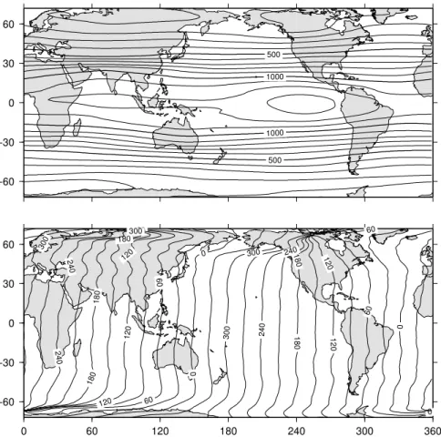
Figure 1 shows the 13-year averaged daily cycle inpa ob-tained by averaging the 12 monthly climatologies. A clear zonal wave number-two pattern, approximately alternating in sign every 6 hours, underlines the dominant presence of the S2tide, but its westward propagation cannot be discerned
from the 6-h maps. The differences in patterns separated by 12 h also hint at the presence of variability associated with the S1 tide. Amplitudes are largest in the tropics and
de-cay to small values at high latitudes. Spatial variations are smooth over the oceans but shorter scale structures appear over land and particularly so over high orography. In gen-eral, the overall characteristics of the ECMWF daily cycle inpa are consistent with past theoretical and observational studies of the air tides (Lindzen, 1990; Dai and Wang, 1999).
ECMWF results are also broadly similar to the climatologies based on the NCEP-NCAR reanalysis (Van den Dool et al., 1997), although ECMWF peak amplitudes are consistently smaller by∼0.5 mb in the tropics.
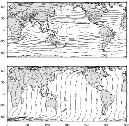
As a preliminary assessment of seasonal effects, Figs. 2 and 3 showpamaps for March and June climatologies, re-spectively. At low latitudes amplitudes are larger in March than in June by∼0.5 mb, indicating a substantial semiannual modulation of the wave number-two pattern associated with S2. Stronger amplitudes in March coincide with the
maxi-mum solar insolation (and thus strongest forcing) over trop-ical regions. Peak amplitudes do not particularly follow the shift in maximum solar insolation from the equator in March to the Tropic of Cancer (23◦N) in June, which is not unex-pected since the atmosphere’s response to radiational forc-ing is dominated by equatorially symmetric modes (Lindzen, 1990). Comparisons between June and December clima-tologies (not shown), nevertheless, indicate that the response over land and land-ocean contrasts are enhanced in the sum-mer hemisphere. Substantial annual modulation of S1signals
over land are, therefore, expected. More detailed discussion of seasonal effects is given below when examining S1 and
S2solutions.
2.2 Time interpolated climatologies
As previously discussed, the 6-h fields in Fig. 1 cannot rep-resent the propagating S2signals. For proper resolution of
the S2tide, we followed essentially the interpolating method
developed by Van den Dool et al. (1997), which implicitly assumes that the barometric tide propagates westward with the Sun at approximately 15◦/h. Merely shifting one pattern by 90◦westward in Fig. 1 does not yield the observed pat-tern 6 hours later, however, partly because of the presence of nonmigrating tidal signals. Nonmigrating components as-sociated with land features and having relatively short spa-tial scales have been noted (Fig.1). To minimize the effects of such signals on the interpolation, at each latitude filter-ing was applied to the climatological fields to retain only the zonal mean plus the first 10 zonal wave numbers, as in Van den Dool et al. (1997). The S2 solutions described below
were not overly sensitive to the filter wave number cutoff and results with more smoothing did not lead to any measurable improvements.
Given the longitudinal grid spacing of 1.125◦, we chose to
R. D. Ray and R. M. Ponte: ECMWF Barometric tides 1899
Fig. 1. Climatological daily cycle of surface pressure (mbar) calculated from 13 years of ECMWF analyses at 00:00, 06:00, 12:00, and
18:00 UT. Negative values are shaded. Contour interval is 0.4 mb.
Fig. 3.As in Fig. 1 but showing climatological daily cycle for June.
To create interpolated values at any timeta+δt in hours, wheretais a time for which an analysis is available, the fol-lowing procedure was applied: (1) the climatological pattern atta was propagated westward by a distance of 15◦×δt to yieldW; (2) the next available climatological pattern atta+6 was propagated eastward by a distance of 15◦×(6 −δt ) to yield E; (3) the two resulting fields were averaged as [(6−δt )×W+δt×E]/6. Interpolated solutions are thus ex-actly equal to the observed (filtered) climatologies at 00:00, 06:00, 12:00, and 18:00 and correspond to a weighted av-erage of the two closest patterns at other times, with prop-agation effects accounted for by the shifting in (1) and (2). Figure 4 shows, as an example, the resulting 13-year average daily cycle inpa at 1.5 h intervals. Thepa patterns exhibit little contamination by short scale land effects and progress smoothly westward in time, as intended.
3 Annual mean S2tide
Global charts of the amplitude and phase of the S2tide can
be readily extracted from the interpolated fields of Fig. 4 by a least-squares fit to a simple sinusoid at every geographic location:
S2(p)=A2cos(2T −ϕ2). (1)
The results are shown in Fig. 5. WithT taken as Univer-sal Time (in appropriate units), the phaseϕis a “Greenwich phase lag” as traditionally employed in ocean-tide studies.
By tracing out successive contours ofϕ, the high-pressure peak of S2(p)can be easily followed in time. Figure 5 shows
it marching westward, leading the Sun by roughly 60◦, or about 2 h, a well-known feature of S2.
Similar figures have been computed from other reanalysis surface pressure fields (e.g. Dai and Wang, 1999; Ray, 2001) and from simulations (e.g. Zwiers and Hamilton, 1986). The annual mean S2tide, derived from the NASA Goddard Earth
Observing System (GEOS-1) reanalysis (Schubert et al., 1993) and from the NCEP-NCAR reanalysis (Kalnay et al., 1996), temporally interpolated by Van den Dool et al. (1997), was extensively compared by Ray (2001). Comparison of Fig. 5 with corresponding NCEP-NCAR and GEOS-1 charts (Figs. 2 and 3 of Ray, 2001) shows gross similarities but also shows some immediate differences. The ECMWF tidal am-plitudes are smaller in the tropical latitudes than NCEP and more zonally symmetric than GEOS-1. The NCEP reanaly-sis amplitudes are thought to be too large (Van den Dool et al., 1997).
More quantitative comparisons and tests of these S2fields
can be obtained by employing the set of “ground truth” S2
R. D. Ray and R. M. Ponte: ECMWF Barometric tides 1901
Fig. 4.Interpolated climatological daily cycle at 1.5 h intervals. Time marches horizontally from the top left corner (00:00 UT) to the bottom
right corner (22:30 UT).
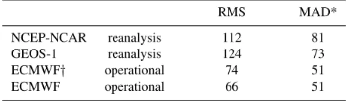
Table 1.S2rms differences (µb) with station estimates
all above latitude ocean
stations 1000 m ≤30◦ stations MAD* NCEP-NCAR reanalysis 151 245 296 208 82 GEOS-1 reanalysis 168 196 300 238 85 ECMWF† operational 124 177 243 211 69 ECMWF operational 112 159 230 134 52 ECMWF(2) operational 110 141 221 156 54
* Median Absolute Difference
†Before phase correction
Of 428 stations, 42 are above 1000 m, 157 are low latitude, 46 are classified oceanic. Solution ECMWF(2) corresponds to Fig. 7.
variability in the tide (see below) can itself produce differ-ences between models and stations, this has been minimized by using, to the greatest extent possible, stations with an integral number of full calendar years (thereby minimizing intra-annual variations) and long multi-year time series
-60 -30 0 30 60
0 60 120 180 240 300 360
0
0
0
0
60
60
60 60 60
120 120
120 120
120
180
180
180
180 180
240 240
240
240
300
300
300
300
-60 -30 0 30 60
500
500 1000
1000
Fig. 5.Amplitude (µb) and Greenwich phase lags (degrees) of the S2(p)tide, calculated as described in the text. The phase contour interval
of 30◦corresponds to 1 h in time.
estimates of S2.
We should stress that Table 1 compares ECMWF opera-tional analysis tides with GEOS and NCEP-NCAR reanal-ysis tides. The difference between meteorological centers is probably less significant than the differences between a reanalysis and a modern analysis, the latter having consid-erably finer resolution in both vertical and horizontal (e.g. T170 vs. T62 grids). In fact, an unpublished study of NCEP operational analysis fields suggests that its tidal signals are more realistic than the NCEP reanalysis (H. Van den Dool, personal communication, 2002).
Figure 6 shows the amplitude and phase differences be-tween the ECMWF tide and each of the 428 station esti-mates, plotted as a function of latitude. Amplitude differ-ences are noticeably larger and more scattered in tropical lat-itudes where the tide itself is maximum. At first glance, and consistent with Table 1, this scatter is less pronounced than in similar diagrams for NCEP and GEOS-1 (Ray, 2001, Figs. 5 and 6). Also noticeable in Fig. 6 (top) is a consistent phase discrepancy between ECMWF and the test stations. Except for a small band near the equator, all latitudes between 60◦N and 60◦S suggest that the ECMWF phasesϕare too large. (Larger phase scatter in high latitudes is of no significance because of the very small amplitudes.) The mean phase dis-crepancy in Fig. 6 is 9.7◦; the median is 10.4◦. A phase error
of 10◦implies that the ECMWF S
2tide is generally too late
by 20 min. Similar phase discrepancies were noticed in the other two reanalysis tides (Ray, 2001), with NCEP too late by roughly 30 min and GEOS-1 too early by roughly 60 min (depending on how the time-tag in the GEOS product is in-terpreted). We are not in a position to offer credible explana-tions for the cause of such time discrepancies, except to say that they appear to be fairly robust (as in Fig. 6) and that the errors cannot be in the station data. The statistics of Table 1 show the model-station comparisons both before and after the model phases have been corrected, and the statistics for the corrected phases are lower, as expected. (Both NCEP and GEOS-1 statistics reflect phases already corrected for their deduced systematic errors, as discussed more fully in Ray, 2001.)
A possibly legitimate criticism of Fig. 5 is that the map may be too zonally symmetric, an artifical by-product of the wave number filtering employed by us and by Van den Dool et al. (1997). In fact, examination of the Fig. 1 mean pressures suggests that S2may well embody significant
R. D. Ray and R. M. Ponte: ECMWF Barometric tides 1903 -400 -200 0 200 400 600
Amplitude difference (
µ bar) -80 -60 -40 -20 0 20 40 60 80 Latitude (deg) -150 -100 -50 0 50 100 150
Phase difference (deg)
-80 -60 -40 -20 0 20 40 60 80
Fig. 6.Amplitude and phase differences between ECMWF-implied
S2(p)tide and estimates based on 428 barometer stations. A small
systematic error in the phases is readily apparent.
2001), and which may thus be more realistic in this regard than our Fig. 5. Yet the few features that can be tested by the ground-truth stations suggest that the non-migrating GEOS-1 features must be treated with caution. For example, while the amplitude contours in Fig. 5 are almost perfectly east-west across the North Atlantic Ocean, the GEOS-1 ampli-tudes collapse to a minimum at mid-ocean (Dai and Wang, 1999, Fig. 16); the ground-truth stations, however, suggest no such collapse (Ray, 2001).
Given the 6-h ECMWF sampling, it is impossible to re-cover unambiguously any real non-migrating component of S2. We can, however, restore the non-migrating in-phase
componentA2cosϕ2by fitting a sinusoidal wave to the
dif-ference between our model Eq. (1) and the data of Fig. 1. The modified S2amplitude and phase charts are shown in Fig. 7,
and the relevant ground-truth statistics are listed in Table 1 under the label “ECMWF(2).” According to Table 1 the land regions of the new solution, and especially the high-altitude regions, are more accurate, but the oceanic regions are de-graded, and the overall accuracy is about the same.
4 Annual mean S1tide
Similar charts may be derived for the diurnal S1(p)tide. In
this case, however, it is important to minimize any wave
Table 2.S1differences (µb) with 25 ocean stations
RMS MAD*
NCEP-NCAR reanalysis 112 81 GEOS-1 reanalysis 124 73 ECMWF† operational 74 51 ECMWF operational 66 51
* Median Absolute Difference
†Before phase correction
number filtering because it is well known (Haurwitz and Cowley, 1973) that S1 is dominated by large non-migrating
components with complicated spatial distributions. The S1
tide is evidently susceptable to significant diurnal boundary-layer effects over land masses and land-ocean boundaries. Therefore, we avoid altogether using our temporally interpo-lated fields to deduce S1and return to the original 6-h fields
of Fig. 1, which are sufficient to determine a diurnal wave. At each geographical location we fit to the four mean pres-sure fields (i.e. unfiltered fields at 00:00, 0600, 12:00, and 18:00 UT as given in Fig. 1) a sinusoid of form
S1(p)=A1cos(T −ϕ1). (2)
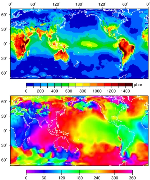
(Oceanographers usually add 180◦to this argument.) The re-sulting amplitudesA1and phase lagsϕ1are shown in Fig. 8.
The spatial complexity of these fields is highly pronounced relative to the simple semidiurnal wave of Fig. 5. Large non-migrating amplitudes, fixed to certain land features, are clearly apparent. The main migrating component is most ap-parent over the tropical oceans where the phases again show an approximately constant westward march, now lagging the Sun by roughly 250◦, or 17 h (or, equivalently, leading the Sun by roughly 7 h). From Fig. 8 this migrating (zonal wave number-one) component is no more than perhaps half the size of the semidiurnal wave, while the non-migrating compo-nents in some regions (e.g. South America) exceed all semid-iurnal amplitudes.
It would be highly desirable to compare the S1 tide of
Fig. 8 and other reanalysis tides against a “ground truth” data set similar to that used above for S2. Unfortunately, we know
of no similar compilation that is reliable. Our efforts to locate Bernard Haurwitz’s old compilation have so far proven futile. As a makeshift, but limited, test data set we adopt a set of 25 S1station estimates from small oceanic islands (Ray, 1998).
This set of oceanic stations is, of course, completely inade-quate for testing tidal fields over the continents where the S1
signal is largest, but it is nonetheless valuable in two ways: as a test of the predominantly migrating S1component, which
appears to be best isolated in oceanic stations, and as a reli-ability test of the oceanic diurnal pressure forcing for those investigators interested in sea level. Comparisons against this 25-station set of S1 estimates are given in Table 2. The
-60 -30 0 30 60
0 60 120 180 240 300 360
0 0
0
0 60
60
60 60
120 120
120 120
120
180
180
180
180
240 240
240
240 300
300 300
-60 -30 0 30 60
500
500 1000
1000
Fig. 7.Amplitude (µb) and Greenwich phase lags (degrees) of the S2(p)tide, as in Fig. 5, except with the in-phase, non-migrating component
restored. This solution is denoted “ECMWF(2)” in Table 1.
fashion to the S2fields described above, with the NCEP
re-sults based on non-interpolated 6-hour grids.
Our 25-station test set is too limited to allow for a reliable independent estimate of any systematic phase error, as seen above for S2. If the error is caused by a simple time-tag
prob-lem (perhaps related to the times that data are ingested into the analysis), then the observed S2error of 10◦implies a 5◦
error in S1. Applying a 5◦shift to the S1phases does reduce
the rms difference with the 25-station estimates (although the median absolute difference is unchanged). This rms reduc-tion is thus consistent with a 20-min error in the ECMWF pressures.
Table 2 also lists the rms and median absolute differences between the 25 stations and the NCEP and GEOS-1 (reanal-ysis) diurnal tides. As the statistics make clear, the ECMWF (analysis) S1estimates are the most reliable of the three
prod-ucts. We emphasize that this statement applies exclusively to the oceanic regions, since none of the 25 stations is from a continental region.
5 Variability of ECMWF tides
Significant variability in atmospheric tides is a well-known fact (e.g. Chapman and Lindzen, 1970; Haurwitz and Cow-ley, 1973). In this section we examine the nature of this vari-ability as implied by the ECMWF series.
5.1 Monthly analyses
A standard approach to studying variability in atmospheric tides is to concentrate on seasonal variations, either in terms of monthly means or in terms of the so-called Lloyd seasons (winter, summer, equinoctial); see, for example, Chapman and Lindzen (1970). It is straightforward to form monthly estimates of S1(p)and S2(p)from the monthly climatologies
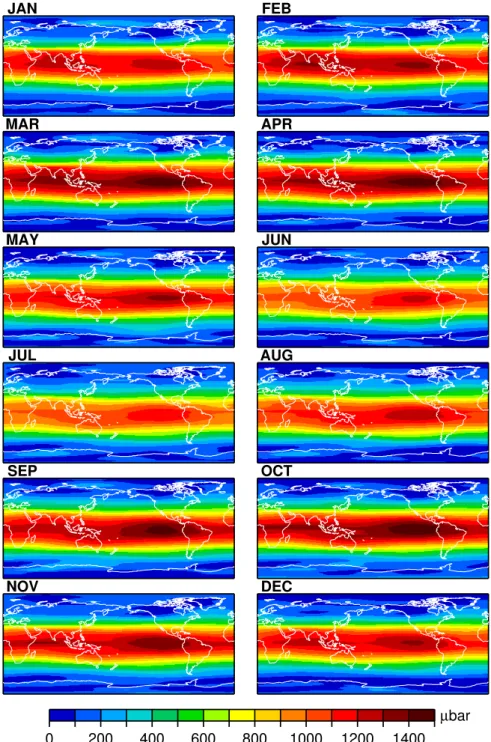
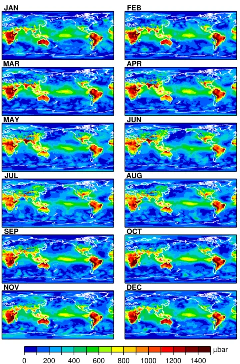
discussed in Sect. 2. Figures 9 and 10 show the resulting amplitudes of both tides.
The annual and semiannual modulations in S2 are very
R. D. Ray and R. M. Ponte: ECMWF Barometric tides 1905
0˚ 60˚ 120˚ 180˚ 120˚ 60˚ 0˚
60˚ 30˚ 0˚ 30˚ 60˚
0 200 400 600 800 1000 1200 1400 µbar
60˚ 30˚ 0˚ 30˚ 60˚
0 60 120 180 240 300 360
Fig. 8.Amplitude and Greenwich phase lags of the S1(p)tide, as deduced from ECMWF surface pressures.
strongest amplitudes during equinoctial months appears to hold also for S1, although this is less obvious because of the
exceedingly complex spatial patterns.
Figures 11 and 12 summarize the tropical responses by de-picting the in-phase and out-of-phase tidal components aver-aged over all tropical regions of the globe. (Such diagrams are essentially equivalent to Chapman’s “harmonic dials”.) To allow for proper zonal averaging of these figures, we have converted all phase lags to correspond to mean local solar time: κn = ϕn +nλ, where λ is east longitude and nis 1 for diurnal and 2 for semidiurnal. (Phases have also been adjusted for the systematic error noted in Fig. 6.) Fig-ure 11 shows an unsymmetrical three-leaf clover pattern for S2, which is consistent with dominant annual and
semian-nual modulations. Again, the smallest amplitudes are clearly in the northern summer months, while northern winter am-plitudes are near the annual mean. Figure 12 separates the tropics into oceanic and land regions because of their dis-similar responses, which is primarily in the large quadrature
A1sinκ1 component (i.e. the component corresponding to
06:00 local time). Smallest amplitudes are again in June and July, but otherwise the oceanic regions are dominated by the annual modulation, whereas the land regions have a strong semiannual modulation with relatively weak amplitudes in January and December.
In passing we might mention that Figs. 11 and 12 show both the strengths and the weaknesses of the Lloyd system of averaging. While the “J season” of May–August gives fairly consistent estimates for all three diagrams, the “D season” of November–February includes a very wide range of phases, if not of amplitudes. Averaging such data into one “season” is of doubtful utility.
5.2 Spectral analysis
JAN FEB
MAR APR
MAY JUN
JUL AUG
SEP OCT
NOV DEC
0 200 400 600 800 1000 1200 1400
µbar
Fig. 9.Monthly mean amplitude of the S2(p)tide as deduced from ECMWF surface pressures.
limitations of using simple monthly means. Wunsch and Stammer (1997) computed the frequency-wave number spec-trum of the ECMWF surface pressures, and we here fol-low up on their work by studying in more detail the spectral structure near the tidal peaks. Wunsch and Stammer display the two-dimensional spectrum, which we need not repro-duce here. The two-dimensional spectrum may be summed over all wave numbers to yield a simple one-dimensional fre-quency spectrum representative of the global pressure field (for details, although in an oceanographic context, see Wun-sch and Stammer, 1995).
Figure 13 shows the frequency spectrum estimated from four full years of six-hourly ECMWF surface pressures (years 1996–1999). Although no spectral smoothing has been performed, the spectrum is still relatively smooth be-cause summation over all wave numbers significantly re-duces random noise, thus allowing the delineation of some very subtle spectral features. There are clear peaks at the an-nual (0.0027 cpd) and semi anan-nual (0.0055 cpd) frequencies and at the S1 and S2 tidal frequencies, the latter occurring
R. D. Ray and R. M. Ponte: ECMWF Barometric tides 1907
JAN FEB
MAR APR
MAY JUN
JUL AUG
SEP OCT
NOV DEC
0 200 400 600 800 1000 1200 1400
µbar
Fig. 10.Monthly mean amplitude of the S1(p)tide as deduced from ECMWF surface pressures.
small peaks between the two tidal frequencies; close exam-ination shows them occurring at frequencies 1.314, 1.628, 1.685, and 1.932 cpd. The latter is the expected lunar tide M2, but the others are unexpected and correspond to no tidal
or modal period that we are aware of (e.g. Hamilton and Gar-cia (1986) find several modal peaks in the Batavia pressure spectrum but none corresponds to Fig. 13 frequencies). The first two peaks are apparent harmonics of an S1modulation,
since they are equidistant from 1.0 cpd. Our conjecture is that these peaks are likely spurious, related to some feature of the ECMWF processing.
Figure 14 is a “zoom” view of Fig. 13 near 1 and 2 cpd.
One sees the detailed fine structure around the tidal peaks (the fundamental spectral resolution here is 0.25 cpy). There is a clear, broad cusp of enhanced energy surrounding both tidal peaks. This cusp spans a frequency range of roughly ±0.01 cpd on either side of the main spectral line. In addition to the cusp, and most prominent in S1, there are modulations
of the main peaks at integral multiples of once per year. For S1the annual modulations are relative strong, each
represent-ing about a tenth of the energy of the main line. This is con-sistent particularly with the oceanic regions of Fig. 12. For S2only the semiannual modulation is apparent; if an annual
Presum--1200 -1150 -1100 -1050 -1000 -950 -900 -850
Quadrature component (
µ
bar)
250 300 350 400 450 500 550
In phase component (µbar)
1 2 3 4 5 6 7 8 9 10 11 12
S
2Fig. 11.Monthly estimates of the in-phase(A2cosκ2)and
quadra-ture(A2sinκ2) components of the S2(p)tide, averaged over all
tropical regions (latitudes≤23◦). Months are labeled 1–12.
Table 3.Integrated energy in tidal bands, Pa2
S1 S2
Primary line 1070 3300 Secondary sideline(s) 120 30 Incoherent cusp 310 500
ably the S2tide has a similar structure above the Nyquist
fre-quency, which is folded back into frequencies below 2 cpd. Table 3 summarizes the integrated spectral densities over the appropriate frequency ranges that surround the tidal peaks of Fig. 14. In both diurnal and semidiur-nal cases, the cusps represent comparable energy, about (0.2 mb)2, while the modulating sidelines represent signifi-cantly smaller amounts, although more in the diurnal band than semidiurnal. In relation to the main peak, variability is more important for the diurnal tide. (Note that the values for the main peaks in Table 3 are reasonably consistent with the global S2 and S1 amplitude fields shown in Figs. 5 and 8,
respectively: for these fields the rms over a complete tidal cycle is 570µb for S2, corresponding to a variance of 3300
Pa2, and 315µb for S1, corresponding to a variance of 1000
Pa2.)
From Fig. 14 we conclude that the ECMWF tides display modulations at once and twice per year (and even tiny further peaks at 3, 4, and 5 times per year), but that these modula-tions are dominated by a complex cusp of incoherent, essen-tially stochastic, energy that complicates the development of simple models. For example, the monthly means of Figs. 9 and 10 could be adequately represented by an annual modu-lation and a few higher harmonics, but such a model would
850 900 950 1000 1050
Quadrature component (
µ
bar)
0 50 100 150
In phase component (µbar) 1 2 3 4 5 6 7 8 9 10 11 12 Tropical Land
S
1 300 350 400Quadrature component (
µ
bar)
0 50 100 150
In phase component (µbar) 1 2 3 4 5 6 7 8 9 10 1112 Tropical Ocean
S
1Fig. 12. As in Fig. 11 but for S1(p), and separated into tropical
ocean and land regions.
fail to capture the majority of the tidal variability that resides within the cusps.
6 Summary remarks
Thirteen years of operational ECMWF fields were used to construct monthly climatologies of the daily cycle in surface pressure for the study of the S2(p)and S1(p)tides.
Com-parisons with station pressure data and products from other weather centers showed that the S2(p)and S1(p)tides are
well represented in the ECMWF analysis. The available 6-hourly fields sample the S2tide at its Nyquist frequency, but
our findings indicate that simple time interpolation schemes, as proposed by Van den Dool et al. (1997) and used here, can work well in extracting the propagating S2 tide. The
R. D. Ray and R. M. Ponte: ECMWF Barometric tides 1909 10-2 10-1 10-1 100 101 102 103 104
Spectral density (mbar
2/cpd)
10-3 1010-2-2 10-1 100
Frequency (cpd)
Fig. 13. Globally integrated spectrum of the ECMWFpa series,
based on the four-year span 1996–1999. For computational details, see Wunsch and Stammer (1995).
relative to the observations. Such a shift in time can be eas-ily corrected a posteriori, but the reasons behind it remain unclear.
Analyses of the monthly climatologies and four years (1996–1999) of 6-h fields revealed a complex, seasonal mod-ulation of the tides superimposed on an apparently more im-portant cusp of variability at interannual and other shorter periods. The 4-year series analyzed in Fig. 14 does not per-mit, however, a full evaluation of the interannual and longer period variability of the tides. Furthermore, a strong El Ni˜no occurred in 1997–98 and may have affected the estimated tidal variability at interannual periods in Fig. 14. The study of longer records would be needed to better quantify the vari-ability of the S1 and S2tides, and, in particular, the size of
the annual and semiannual modulations relative to variability at longer periods.
Acknowledgements. P. Nelson (AER) helped with initial process-ing of pressure fields. We thank Huug van den Dool for useful com-ments and discussions. Support for work at AER was provided by NASA Jason-1 Project under contract 1206432 with the Jet Propul-sion Laboratory.
Topical Editor O. Boucher thanks two referees for their help in evaluating this paper.
References
Braswell, W. D. and Lindzen, R. S.: Anomalous short wave absorp-tion and atmospheric tides, Geophys. Res. Lett., 25, 1293–1296, 1998.
Chapman, S. and Lindzen, R.: Atmospheric Tides, Gordan and Breach, New York, 1970.
Chapman, S. and Westfold, K. C.: A comparison of the annual mean solar and lunar atmospheric tides in barometric pressure as regards their worldwide distribution of amplitude and phase, J. Atmos. Terr. Phys., 8, 1–23, 1956.
Cooper, N. S.: Inferring solar UV variability from the atmospheric tide, Nature, 296, 131–132, 1982.
10-2 10-1 10-1 100 101 102 103
Spectral density (mbar
2/cpd)
1.98 1.99 2.00 2.01 2.02
Frequency (cpd) Semidiurnal 10-2 10-1 10-1 100 101 102 103
Spectral density (mbar
2/cpd)
0.98 0.99 1.00 1.01 1.02
Frequency (cpd)
Diurnal
1 cpy
Fig. 14.Detailed views of the spectrum of Fig. 13 surrounding the
diurnal and semidiurnal peaks. Frequency resolution is 0.25 cpy.
Dai, A. and Wang, J.: Diurnal and semidiurnal tides in global sur-face pressure data, J. Atmos. Sci., 56, 3874–3891, 1999. Hamilton, K.: The geographical distribution of the solar
semidi-urnal surface pressure oscillation, J. Geophys. Res., 85, 1945– 1949, 1980.
Hamilton, K.: Quasi-biennial and other long period variations in the solar semidiurnal barometric oscillation: observations, theory, and possible application to the problem of monitoring changes in global ozone, J. Atmos. Sci., 40, 2432–2443, 1983.
Hamilton, K. and Garcia, R. R.: Theory and observations of the short-period normal mode oscillations of the atmosphere, J. Geo-phys. Res., 91, 11 867–11 875, 1986.
Haurwitz, B.: The geographical distribution of the solar semidiurnal pressure oscillation. New York University, College of Engineer-ing, Meteorological Papers, 2, 5, 36 pp, 1956.
Haurwitz, B. and Cowley, A. D.: The diurnal and semidiurnal baro-metric oscillations, global distribution and annual variation, Pure Appl. Geophys., 102, 193–222, 1973.
Hsu, H.-H. and Hoskins, B. J.: Tidal fluctuations as seen in ECMWF data, Q. J. R. Meteorol. Soc., 115, 247–264, 1989. Kalnay, E., Kanamitsu, M., Kistler, R., Collins, W., et al.: The
NCEP/NCAR 40 year reanalysis project, Bull. Am. Met. Soc., 77, 437–471, 1996.
Madden, R. A., Lejen¨as, H., and Hack, J.: Semidiurnal variations in the budget of angular momentum in a general circulation model and in the real atmosphere, J. Atmos. Sci., 55, 2561–2575, 1998. Ponte, R. M.: Variability in a homogeneous global ocean forced by barometric pressure, Dyn. Atmos. Oceans, 18, 209–234, 1993. Ponte, R. M. and Gaspar, P.: Regional analysis of the inverted
barometer effect over the global ocean using TOPEX/ POSEI-DON data and model results, J. Geophys. Res., 104, 15 587– 15 601, 1999.
Ray, R. D.: Diurnal oscillations in atmospheric pressure at twenty-five small oceanic islands, Geophys. Res. Lett., 25, 3851–3854, 1998.
Ray, R. D.: Comparisons of global analyses and station observa-tions of the S2barometric tide, J. Atmos. Solar-Terr. Phys., 63,
1085–1097, 2001.
Schubert, S. D., Rood, R. B., and Pfaendtner, J.: An assimilated data set for earth science applications, Bull. Am. Met. Soc., 74, 2331–2342, 1993.
Van den Dool, H. M., Saha, S., Schemm, J., and Huang, J.: A tem-poral interpolation method to obtain hourly atmospheric surface pressure tides in Reanalysis 1979–1995, J. Geophys. Res., 102,
22 013–22 024, 1997.
Velicogna, I., Wahr, J., and van den Dool, H.: Can surface pres-sure be used to remove atmospheric contributions from GRACE data with sufficient accuracy to recover hydrological signals? J. Geophys. Res., 106, 16 415–16 434, 2001.
Wahr, J., Molenaar, M., and Bryan, F.: Time variability of the Earth’s gravity field: hydrological and oceanic effects and their possible detection using GRACE, J. Geophys. Res., 103, 30 205– 30 229, 1998.
Wilkes, M. V.: Oscillations of the Earth’s Atmosphere, Cambridge Univ. Press, 1949.
Wunsch, C. and Stammer, D.: The global frequency-wave number spectrum of oceanic variability estimated from Topex/Poseidon altimetric measurements, J. Geophys. Res., 100, 24 895–24 910, 1995.
Wunsch, C. and Stammer, D.: Atmospheric loading and the oceanic “inverted barometer” effect, Rev. Geophys., 35, 79–107, 1997. Zwiers, F. and Hamilton, K.: Simulation of solar tides in the