Braz. J. Chem. Eng. vol.29 número3

ISSN 0104-6632 Printed in Brazil

www.abeq.org.br/bjche

Vol. 29, No. 03, pp. 567 - 576, July - September, 2012

Brazilian Journal

of Chemical

Engineering

MATHEMATICAL MODELING OF A

THREE-PHASE TRICKLE BED REACTOR

J. D. Silva

1*

and C. A. M. Abreu

2

1

Polytechnic School, UPE, Laboratory of Environmental and Energetic Technology, Phone: + (81) 3183-7515, Rua Benfica 455, Madalena, CEP: 50750-470, Recife - PE, Brazil.

∗_{E-mail:jornandesdias@poli.br}

2

Department of Chemical Engineering, Federal University of Pernambuco, (UFPE), Phone + (81) 2126-8901, R. Prof. Artur de Sá 50740-521, Recife - PE Brazil.

E-mail:cesar@ufpe.br

(Submitted: August 5, 2010 ; Revised: July 27, 2011 ; Accepted: April 16, 2012)

Abstract - The transient behavior in a three-phase trickle bed reactor system (N2/H2O-KCl/activated carbon,

298 K, 1.01 bar) was evaluated using a dynamic tracer method. The system operated with liquid and gas phases flowing downward with constant gas flow QG = 2.50 x 10-6 m3 s-1 and the liquid phase flow (QL)

varying in the range from 4.25x10-6 m3 s-1 to 0.50x10-6 m3 s-1. The evolution of the KCl concentration in the aqueous liquid phase was measured at the outlet of the reactor in response to the concentration increase at reactor inlet. A mathematical model was formulated and the solutions of the equations fitted to the measured tracer concentrations. The order of magnitude of the axial dispersion, liquid-solid mass transfer and partial wetting efficiency coefficients were estimated based on a numerical optimization procedure where the initial values of these coefficients, obtained by empirical correlations, were modified by comparing experimental and calculated tracer concentrations. The final optimized values of the coefficients were calculated by the minimization of a quadratic objective function. Three correlations were proposed to estimate the parameters values under the conditions employed. By comparing experimental and predicted tracer concentration step evolutions under different operating conditions the model was validated.

Keywords: Trickle Bed; KCl Tracer; Modeling; Transient; Validation.

INTRODUCTION

Mathematical modeling of three-phase trickle bed reactors (TBR) considers the mechanisms of forced convection, axial dispersion, interphase mass transport, intraparticle diffusion, adsorption and chemical reaction. These models are formulated by relating each phase to the others (Silva et al., 2003; Iliuta et al., 2002; Latifi et al., 1997; Burghardt et al., 1995).

The trickle-bed reactor is a three-phase catalytic reactor in which liquid and gas phases flow concurrently downward through a fixed bed of solid catalyst particles where the reactions take place. These systems have been extensively used in

hydrotreating and hydrodesulfurization in petroleum refining, petrochemical hydrogenation and oxidation processes, and methods of biochemical and detoxification of industrial waste water (Al-Dahhan et al., 1997; Dudukovic et al., 1999; Liu et al., 2008; Ayude et al., 2008; Rodrigo et al., 2009; Augier et al., 2010).

The purpose of this work was to evaluate the transient behavior of a three-phase trickle bed reactor using a dynamic tracer method to estimate the magnitude of the hydrodynamic parameters related to the operations, including the axial dispersion coefficient in the liquid phase, the liquid-solid mass transfer coefficient and the partial wetting efficiency. A dynamic phenomenological model was proposed and validated with experimental reaction data.

MATHEMATICAL MODEL

To represent the dynamic behavior of the tracer component, a one-dimensional mathematical model was formulated considering the effects related to the axial dispersion, liquid-solid mass transfer, partial wetting and chemical reaction. The model was adopted for KCl, considered to be the tracer component in the liquid phase, and was restricted to the following hypotheses: (i) isothermal operation; (ii) constant gas and liquid flow rates throughout the reactor; (iii) moderate intraparticle diffusion resistance; (iv) the chemical reaction rate within the catalytic solid is equal to the liquid-solid mass transfer rate, in any position of the reactor. The mass balance for the tracer (AL) in the liquid phase is written as:

Mass balance for the liquid;

( )

( )

( ) ( )

( )

( )

L L

d,L SL

2 L

ax ₂ s M LS LS

L S

A z, t A z, t

H V

t z

A z, t

D 1 F k a

z

A z, t A z, t

∂ ₊ ∂ ₌

∂ ∂

∂ _{− − ε}

∂ −

⎡ ⎤

⎣ ⎦

(1)

The initial and boundary conditions for Eq. (1) are given as:

( )

L L,0

A z,0 =A ; for all z (2)

( )

_{( )}

_{( )}

L SL

L _{z 0} L

ax z 0

A z, t V

A z, t A z,0

z ₌ + D = +

∂ _{= ⎡ − ⎤}

⎢ ⎥

⎣ ⎦

∂ ,

(3) for t > 0

( )

L

z L A z, t

0

z ₌

∂ ₌

∂ ; for t > 0 (4)

The equality of the mass transfer and reaction rates can be expressed by the following equations:

( )

( )

M LS LS L S S S KCl

F k a ⎡_⎣A z, t −A z , t ⎤_⎦= η ε r (5)

The kinetic model for the reaction was based on a first-order reaction according to the following expression (Colombo et al., 1976):

( )

KCl r s

r =k A z, t (6)

where rKCl is the consumption rate of the reactant, As(z, t) is the reactant concentration at the surface of the solid phase and kr is the reaction rate constant of the first-order reaction.

Combining Equations (5) and (6), the rate of mass transfer is equal the rate of reaction at the surface of the solid phase as:

( )

( )

( )

M LS LS L S

r S S S

F k a A z, t A z , t

k A z , t

− =

⎡ ⎤

⎣ ⎦

η ε (7)

Equations (1) to (4) and (7) can be analyzed by employing the dimensionless variables in Table 1.

Table 1: Summary of dimensionless variables

Dimensionless concentrations

dimensionless variables

( ) L( ) L d

L,0

A z, t , t

A

ψ ξ = SL

d d,L

V t

t L H

=

( ) S( ) S d

L,0

A z, t , t

A

ψ ξ = z

L

ξ =

Expressed in the dimensionless variables, the equations and the initial and boundary conditions can be rewritten as:

( )

( )

( )

( )

( )

2

L d L d L d

2

d E

LS L d S d

, t , t 1 , t

t P

, t , t

∂ψ ξ ₊∂ψ ξ ₌ ∂ ψ ξ ₋

∂ ∂ξ ∂ξ

α ⎡_⎣ψ ξ − ψ ξ ⎤_⎦ (8)

( )

L ,0 1

ψ ξ = ; for all ξ (9)

( )

_{( )}

L d

E L d ₀

0 , t

P , t ₊ 1

+ ξ=

ξ=

∂ψ ξ _{= ⎡ψ ξ − ⎤}

⎢ ⎥

⎣ ⎦

∂ξ ;

( )

L d 1 , t 0 ξ =

∂ψ ξ ₌

∂ξ for td> 0 (11)

( )

( )

( )

L , td S , td S S , td

ψ ξ − ψ ξ = β ψ ξ (12)

Equations (8) to (12) include the following dimensionless parameters:

(

s

)

M LS LS LS

SL

1 F k a L

V

− ε

α = (13)

SL E ax V L P D

= (14)

r s s S

LS LS M k

k a F

η ε

β = (15)

The dimensionless concentration, ψS (ξ, td), was isolated in Eq. (12) and introduced into Eq. (8), reducing it to:

(

)

(

)

(

)

₍

₎

L d L d

d 2 L d L d 2 E

, t , t

t

, t 1

, t P

∂ ψ ξ ₊ ∂ ψ ξ ₌

∂ ∂ ξ

∂ ψ ξ _{− γ ψ ξ}

∂ ξ (16) where, LS S S 1 α β

γ = _{β +} (17)

SOLUTION IN THE LAPLACE DOMAIN

Applications of the Laplace Transform (LT) to dynamic transport problems in three-phase trickle bed reactors with tracer (liquid, gas) are employed to solve the linear differential equations. To complete the solution, the Laplace Transform inversion method is indicated, where numerical inversion is often employed. In the present work, the LT technique was applied to the partial differential equation, Eq. (16), as presented below:

( )

( )

( ) ( )

2 L L E 2 E E L

d ,s d ,s

P d d

P

P s ,s

s

ψ ξ ₋ ψ ξ ₋

ξ ξ

+ γ ψ ξ = −

(18)

where the overhead bar (−) and “s” indicate the LT and its domain variable, respectively.

The initial and boundary conditions in the Laplace domain are:

( )

L

1 ,s

s

ψ ξ = (19)

( )

_{( )}

L

E L

d 0,s 1

P 0,s

d s

ψ ₌ ⎡_{ψ −} ⎤

⎢ ⎥

ξ ⎣ ⎦ (20)

( )

L d 1,s 0 d ψ ₌

ξ (21)

Eq. (18) is a second-order non-homogeneous ordinary differential equation. Its solution is expressed by Eq. (22) and is composed of the general solution of the homogeneous ordinary differential equation

( )

L, h ,s

ψ ξ and a particular solution ψ_{L, p}

( )

ξ,s :

( )

( )

( )

L,g ,s L, h ,s L, p ,s

ψ ξ = ψ ξ + ψ ξ (22)

The second-order homogeneous ordinary differential equation is expressed as:

( )

( )

( ) ( )

2 L L E 2 E L

d ,s d ,s

P d d

P s ,s 0

ψ ξ ₋ ψ ξ ₋

ξ ξ

+ γ ψ ξ = (23)

Its general solution is given by the following function:

( )

( )

_{( )}

2( )_{( )} 1 2 s 1 L,h s 2 C s e

,s e

C s e

β ξ

β ξ

−β ξ

⎡ ₊⎤

ψ ξ = ⎢ ⎥

⎢ ⎥

⎣ ⎦ (24)

where β1 and β2(s) are defined as:

1 E

1 P 2

β = ,

( )

( )

( )

1 2 2

2 E E

1

s P 4 P s

2

⎡ ⎤

β = _⎢ + + γ _⎥

⎣ ⎦

In term of hyperbolic functions, Eq. (24) was written as:

( )

1 1

_{( )}

( )

2

_{( )}

( )

L,h

2 2

f s sinh s

,s e

f s cosh s

β ξ⎡ β ξ +⎤

ψ ξ = _{⎢ β ξ ⎥}

⎣ ⎦ (25)

where f1(s) and f2(s) are expressed by

( )

( )

( )

1 1 2

The particular solution was given by the expression:

( ) ( )

L, P 1 ,s s s

ψ ξ = _{+ γ} (26)

The general solution has been presented as Eq. (22), in which ψ_{L, h}

( )

ξ,s and ψ_{L, P}

( )

ξ,s were attributed according to the result below:

( )

( )

_{( )}

( )

_{( )}

(

)

1 1 2

L,G

2 2

f s sinh s ,s e

f s cosh s 1

s s

β ξ⎡ β ξ+⎤

ψ ξ = _{⎢ β ξ ⎥}+

⎣ ⎦

+ γ

(27)

where f1(s) and f2(s) are two arbitrary integration constants. Applying the boundary conditions from Eqs. (20) and (21) to the general solution, Eq. (27), led to the algebraic equations needed to find the arbitrary integration constants f1(s) and f2(s) in terms of known parameters. The expressions for these two constants have been found here as:

( )

( )

_{( )}

( )

( )

( )

( )

E L

1 _{2 2}

1 2

2 2 1 2

2

P s 0,s 1

f s

s s

s sinh s cosh s

sinh s ψ − ⎡ ⎤ ⎣ ⎦ = − _{⎡ ⎤} β −β ⎣ ⎦

β β + β β

⎡ ⎤ ⎣ ⎦ β (28)

( )

( )

_{( )}

( )

( )

( )

( )

E L

2 _{2 2}

1 2

2 2 1 2

2

P s 0,s 1

f s

s s

s cosh s sinh s

sinh s

ψ −

⎡ ⎤

⎣ ⎦

=

⎡β −β ⎤

⎣ ⎦

β β + β β

⎡ ⎤

⎣ ⎦

β

(29)

Eqs. (28) and (29) were introduced into Eq. (27) to obtain the general solution of the tracer concentration in the liquid phase:

( )

_{( )}

( )

_{( )}

( )

( )

( )

( )

( )

( )

( )

( )

( )

1 E L

L,G _{2 2}

1 2 2

2 2 1 2 2

2 2 1 2 2

e P s 0,s 1

,s

s s sinh s

s sinh s cosh s sinh s

s cosh s sinh s cosh s

1 s s

β ξ _{⎡ ψ − ⎤}

⎣ ⎦

ψ ξ =

⎡β −β ⎤ β

⎣ ⎦

⎧− β⎡_⎣ β +β β ⎤_⎦ β ξ+⎫₊

⎨ _{⎡β β +β β ⎤ β ξ} ⎬

⎣ ⎦

⎩ ⎭

+γ

(30)

For ξ = 1 it was possible to obtain the concentration of the tracer at the exit of the fixed bed as follows:

( )

1

( ) ( )

L,G L,G

0

s ,s 1 d

ξ = ξ=

ψ =

∫

ψ ξ δ ξ− ξ (31)

Hence,

( )

( )

_{( )}

( )

( )

( )

( )

{

}

(

)

1 E L

L,G _{2 2}

1 2

2 2 2 2

e P s s 1

s

s s

s cosh s coth s sinh s

1 s s

β _{⎡ φ − ⎤}

⎣ ⎦

ψ =

⎡β − β ⎤

⎣ ⎦

β ⎡_⎣ β β − β ⎤_⎦ +

+ γ

(32)

To obtain the concentration evolution of the tracer at the exit of the trickle-bed reactor, the numerical fast Fourier transform (NFFT) technique was employed. In the NFFT operations, the Laplace variable “s” was changed to “ωi” in the Fourier domain. This technique was applied considering a step concentration disturbance at the inlet of the fixed bed, whose expression is written as:

( )

_{( )}

_{( )}

Cal. 1 ax, LS

L,G d L,G

M

D k ,

1

t TF

F , i

i

− ⎧⎪ ⎡ ⎤⎫⎪

ψ = ⎨ _ω ψ _{⎢⎣ ω ⎥⎦}⎬

⎪ ⎪

⎩ ⎭ (33)

MATERIAL AND METHODS

Continuous analysis of the KCl tracer, fed at the reactor top at a concentration of 0.05M, was performed by using a refractive index detector (HPLC detector, Varian ProStar) at the exit of the fixed bed. The results were expressed in terms of the tracer concentration versus time.

The methodology applied to evaluate the order of magnitude of the axial dispersion, liquid-solid mass transfer coefficient and the partial wetting efficiency for the N2/H2O-KCl/activated carbon system was:

ƒ Comparison of the experimental concentrations with the predicted concentrations based on the solutions of Eq. (33), developed for the system;

ƒ Evaluation of the initial values of the parameters

Dax, kLS and FM from the correlations in Table 2;

ƒ Numerical optimization of the values of the model parameters employing, as the criterion, the minimization of a quadratic objective function expressed in terms of experimental and calculated concentrations, given by Eq. (34):

(

)

( )

( )

2

Exp.

N L,G d _k

ax LS M

Cal. k 1

L,G d _k t F D , k , F

t

=

⎧ _{⎡ψ ⎤ −}⎫

⎣ ⎦

⎪ ⎪

⎪ ⎪

= _{⎨ ⎬}

⎪ _{⎡⎣ψ ⎤⎦} ⎪

⎪ ⎪

⎩ ⎭

∑

(34)

The operating conditions and the characteristics of the trickle-bed system are presented in Table 3.

Table 2: Correlations for parameter estimation. Initial values of Dax, kLS and FM.

Correlations References

( )0.61

ax L

D =0.55 Re Lange et al. (1999)

( )LS ( )SL

ln k =1.43+0.92 ln V Tsamatsoulis and Papayannakos (1995)

( )0.22( ) 0.08( ) 0.51

M L G L

F =3.40 Re Re − Ga − Burghardt et al. (1990)

Table 3: Summary of operating conditions in the trickle-bed system (Colombo et al_{., 1976; Silva} et al_.,

2003).

Category Properties Numerical Values

Pressure (P), bar 1.01

Temperature (T), K 298.00

Liquid flow (Qg)x106, m3 s-1 2.50

Gas flow (Ql)x106, m3 s-1 4.25-0.5

Operating Conditions

Standard acceleration of gravity (g)x10-1_{, m s}-2 _9.81

Total bed height (L)x102_{, m 22.0}

Bed porosity (εp) 0.59

Effective liquid-solid mass transfer area per unit column volume (aLS)x10-2, m2 m-3 3.97

Diameter of the catalyst particle (dp)x104, m 4.50

Diameter of the reactor (dr)x102, m 3.00

Density of the particle (ρp)x10-3, kg m-3 2.56

Reaction rate constant (kr)x103, kgmol kg-1 s-1 6.33

Packing and bed properties

Catalytic effectiveness factor (ηS) 0.89

Density of the liquid phase (ρl)x10-3, kg m-3 1.01

Viscosity of the liquid phase (μl)x10-4, kg m-1 s-1 8.96

Surface tension (σl)x102, kg s-2 7.31

Dynamic liquid holdup (hd,l)x101 4.91

Liquid properties

Superficial velocity of the liquid phase (VSL)x104, m s-1 1.56

Density of the gaseous phase (ρg)x101, kg m-3 6.63

Viscosity of the gaseous phase (μg)x105, kg m-1 s-1 1.23

Gas properties

RESULTS AND DISCUSSION

Experiments were performed at constant gas flow QG = 2.50 x 10-6 m3 s-1 and with the liquid phase flow (QL) varying in the range from 0.50x10-6 m3 s-1 to 4.25x10-6 m3 s-1. The experiments carried out with liquid phase flows of (0.50, 0.75, 1.25, 1.75, 2.25, 2.75, 3.25, 3.75, 4.25)x10-6 m3 s-1 were employing to fit the model equations, while operations with liquid phase flows of (1.00, 1.50, 2.00, 2.50, 3.00, 3.50, 4.00)x10-6 m3 s-1 were used for the model validation. Corresponding to the gas and liquid phase flows, the following superficial velocities were employed in the model equations: for the gas phase (nitrogen), VSG was maintained at 10-3 m s-1, and for the liquid aqueous solution of KCl, VSL ranged from 2 x 10-4 m s-1 to 45 x 10-4 m s-1.

The values of the axial dispersion, the liquid-solid mass transfer coefficient and the partial wetting efficiency were determined simultaneously by comparing experimental and predicted concentration data obtained at the exit of the fixed bed, subject to the minimization of the quadratic objective function (F), Eq. (34).

The numerical procedure used to optimize the values of the parameters involved the solution of Eq. (34) associated with an optimization subroutine (Silva et al., 2003, Box, 1965). The procedure started with initial values of the parameters until the final values were obtained, considered to be the optimized values of the three parameters when the quadratic objective function was minimized. The magnitudes of the parameters at different liquid phase flows are reported in Table 4.

Table 4: Optimized values of the parameters axial dispersion, liquid-solid mass transfer coefficient and wetting efficiency. Conditions: N2/H2O-KCl/ activated carbon, 298 K, 1.01 bar, QG = 2.50x10-6 m3 s-1.

Liquid Phase Flows

Optimized Values

Objective Function

QL x

106 _m3 _s-1

Dax x

107 _m2 _s-1

kLS x

106 _{m s}-1 FM F x 104

4.250 6.986 6.109 0.581 2.974

3.750 6.038 5.108 0.573 2.832

3.250 5.107 4.163 0.564 2.739

2.750 4.201 3.275 0.554 2.643

2.250 3.321 2.461 0.544 2.536

1.750 2.475 1.718 0.529 2.456

1.250 1.669 1.061 0.511 2.399

0.750 0.918 0.512 0.485 2.271

0.500 0.572 0.286 0.465 2.179

The axial dispersion, the liquid-solid mass transfer coefficient and the wetting efficiency are

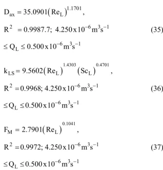
influenced by changes in the liquid flow. To represent the behavior of Dax, kLS and FM, their optimized values were employed and empirical correlations formulated as Eqs. (35), (36) and (37). These are restricted to the following operational conditions:

dP = 3.90 x10-4, 1.49 ≤ ReL≤ 1.75, 0.90 ≤ ScL≤ 4.22.

( )

1.1701

ax L

2 6 3 1

6 3 1 L

D 35.0901 Re ,

R 0.9987.7; 4.250 x10 m s Q 0.500 x10 m s

− −

− −

= =

≤ ≤

(35)

( )

1.4303

( )

0.4701

LS L L

2 6 3 1

6 3 1 L

k 9.5602 Re Sc ,

R 0.9968; 4.250 x10 m s Q 0.500 x10 m s

− −

− −

= =

≤ ≤

(36)

( )

0.1041

M L

2 6 3 1

6 3 1 L

F 2.7901 Re ,

R 0.9972; 4.250 x10 m s Q 0.500 x10 m s

− −

− −

= =

≤ ≤

(37)

The parameter correlations were fitted by the least-squares method. The mean relative errors (MRE) between the predicted and experimental parameter values of Dax, kLS and FM in the k experiments were computed as follows:

( )

( )

( )

Pred. Exp. Exp.

n

k k

k 1

k

p p

1

MRE(p) x 100;

n _{= p}

−

=

∑

ax LS M

p=D ,k and F . Figures 1, 2 and 3 present parity plots of the correlated results. The mean relative errors of Dax, kLS and FM at different liquid flows are shown in Table 5.

Table 5: Mean relative errors of Dax, kLS and FM at different liquid flows

MREDax (%) MREkLS (%) MREFM (%)

0.0 1.5 3.0 4.5 6.0 7.5 0.0

1.5 3.0 4.5 6.0 7.5

-5% +5%

(D_ax)Pred.x107m2s-1

(D

ax

)

E

x

p

. x10 7 m 2 s

-1

0.0 1.6 3.2 4.8 6.4

0.0 1.6 3.2 4.8 6.4

-5% +5%

(k

LS) Pred.

x106m3s-1 (kL

S

)

E

xp.

x1

0

6 m 3 s

-1

Figure 1: Parity (Dax)Exp versus (Dax)Calc for the system N2/H2O-KCl/activated carbon operating in the low interaction regime. Conditions: 298 K, 1.01 bar, QG = 2.50 x 10-6 m3s-1, QL = (4.25 to 0.50) x 10-6 m3s-1 according to Table 4.

Figure 2: Parity (kLS)Exp versus (kLS)Calc for the system N2/H2O-KCl /activated carbon operating in the low interaction regime. Conditions: 298 K, 1.01 bar, QG = 2.50 x 10-6 m3s-1, QL = (4.25 to 0.50) x 10-6 m3s-1 according to Table 4.

0.45 0.48 0.51 0.54 0.57 0.60 0.45

0.48 0.51 0.54 0.57 0.60

(FM

)

E

xp.

(F

M) Pred

-5% +5%

Figure 3: Parity (FM)Exp versus (FM)Calc for the system N2/H2O-KCl /activated carbon operating in the low interaction regime Conditions: 298 K, 1.01 bar, QG = 2.50 x 10-6 m3s-1, QL = (4.25 to 0.50) x 10-6 m3s-1 according to Table 4.

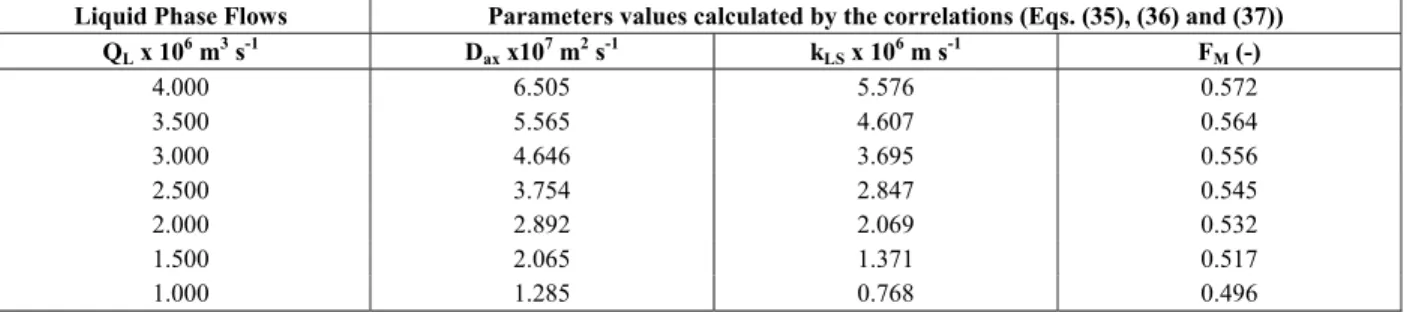
A model validation procedure was established by comparing the predicted concentrations obtained with the values of the parameters from the proposed correlations (Eqs. (35), (36) and (37)) and experimental data not employed in the model adjustment. Table 6

presents the values of the parameters.

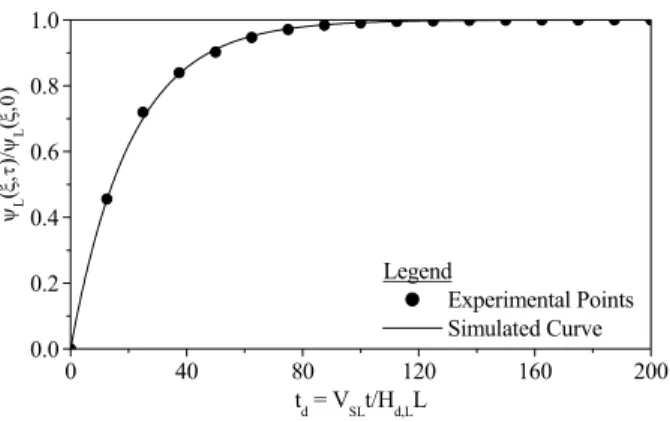
Figures 4 to 6 represent the model validations for three different operating conditions, where the parameter values were obtained from Eqs. (35), (36) and (37).

Table 6: Values of the axial dispersion, liquid-solid mass transfer coefficient and wetting efficiency applied to the model validation. Conditions: N2/H2O-KCl/activated carbon, 298 K, 1.01 bar, QG = 2.50 x 10-6 m3 s-1

Liquid Phase Flows Parameters values calculated by the correlations (Eqs. (35), (36) and (37))

QL x 106 m3 s-1 Dax x107 m2 s-1 kLS x 106 m s-1 FM (-)

4.000 6.505 5.576 0.572

3.500 5.565 4.607 0.564

3.000 4.646 3.695 0.556

2.500 3.754 2.847 0.545

2.000 2.892 2.069 0.532

1.500 2.065 1.371 0.517

0 40 80 120 160 200 0.0

0.2 0.4 0.6 0.8 1.0

Legend

Experimental Points Simulated Curve ψL

(

ξ,τ

)/

ψL

(

ξ,

0

)

t_d = V_SLt/H_d,LL

0 40 80 120 160 200

0.0 0.2 0.4 0.6 0.8 1.0

t_d = V_SLt/H_d,LL Legend

Experimental Points Simulated Curve ψL

(

ξ,τ

)/

ψL

(

ξ,

0

)

Figure 4: Evolution of the tracer concentration at the outlet of the trickle-bed reactor. Model validation. Conditions: 298 K, 1.01 bar, QG = 2.50 x 10-6m3 s-1, QL = 1.50 x 10-6m3 s-1, Dax = 2.065 x 10-7 m2s-1, kLS = 1.371 x 10-6 m s-1 and FM = 0.517

Figure 5: Evolution of the tracer concentration at the outlet of the trickle-bed reactor. Model validation. Conditions: 298 K, 1.01 bar, QG = 2.50 x 10-6m3 s-1, QL = 2.50 x 10-6m3 s-1, Dax = 3.754 x 10-7 m2s-1, kLS = 2.847 x 10-6 m s-1 and FM = 0.545

0 40 80 120 160 200

0.0 0.2 0.4 0.6 0.8 1.0

td = VSLt/Hd,LL ψL

(

ξ,

τ

)/

ψL

(

ξ,

0

)

Legend

Experimental Points Simulated Curve

Figure 6: Evolution of the tracer concentration at the outlet of the trickle-bed reactor. Model validation. Conditions: 298 K, 1.01 bar, QG = 2.50 x 10-6m3 s-1 and QL = 3.50 x 10-6m3 s-1, Dax = 5.565 x 10-7 m2s-1, kLS = 4.607 x 10-6 m s-1 and FM = 0.564

CONCLUSIONS

The transient behavior of the three-phase trickle bed system N2/H2O-KCl/activated carbon was evaluated via an experimental dynamic method and via predictions of a phenomenological mathematical model. Operating at 298 K under 1.01 bar with liquid and gas phases flowing downward under constant gas flow QG = 2.50 x 10-6 m3 s-1 and the liquid phase flow (QL) varying in the range from 4.25x10-6 m3 s-1 to 0.50x10-6 m3 s-1, the concentration of KCl was measured at the exit of the reactor in response to a concentration step at the reactor inlet.

The solutions of the model equations predicted concentration profiles of the tracer employing optimized values of the parameters for the axial dispersion coefficient in the liquid phase, the liquid-solid mass transfer coefficient and the partial wetting efficiency. The magnitudes of the parameters were in the following ranges: Dax = 6.986 x 10-7 m2 s-1 to

0.572 x 10-7 m2 s-1, kLS = 6.109 x 10-6 m s-1 to 0.286 x 10-6 m s-1 and FM = 0.581 to 0.465. These results led to the proposal of three empirical correlations to quantify the influence of liquid phase flow rate changes on the axial dispersion, liquid-solid mass transfer and wetting efficiency in the low interaction regime.

Based on the values of the parameters indicated by the correlations, the model was validated by comparing their predictions with those obtained in different three-phase operations with mean quadratic deviations between experimental and predicted concentrations on the order of 10-4.

ACKNOWLEDGMENTS

NOMENCLATURE

AL(z,t) Concentration of the tracer in the liquid phase

kg m-3 AS(z,t) Concentration of the tracer

on the external surface of solid

kg m-3

aLS Effective liquid-solid mass transfer area per unit

column volume

m2 m-3

Dax Axial dispersion coefficient for the tracer in the liquid phase

m2 s-1

dP Diameter of the catalyst particle

m

dr Diameter of the reactor m

F Quadratic objective function

FM wetting factor dimensionless

GaL Galileo number

L

3 2

a p L L

G =d gρ μ

Hd,L Dynamic liquid holdup dimensionless i _{Complex number −1}

kr Reaction constant kgmol kg-1 s-1

L Height of the catalyst bed m

PE Peclet number PE =VSL L / Dax

QG Gas phase flow m3 s-1

QL Liquid phase flow m3 s-1

ReL Reynolds number ReL=VSLρL dR / μL ScL Schmidt number ScL=μL / ρL Dax

t Time s

VSG Superficial velocity of the gas phase

m s-1 VSL Superficial velocity of the

liquid phase

m s-1 z Axial distance of the

catalytic reactor

m

Greek Letters

αLS Parameter defined in Eq. (13) dimensionless

βS Parameter defined in Eq. (15) dimensionless

εP internal porosity dimensionless

Ψi (ξ,td) Dimensionless

concentration of the tracer in liquid and solid

i = L, S

( )

L,G s

ψ Dimensionless

concentration of the tracer in liquid in the Laplace domain

η Catalytic effectiveness factor

ρL Density of the liquid phase kg m -3

μL Viscosity of the liquid phase

kg m-1 s-1

REFERENCES

Al-Dahhan, M. H., Larachi, F., Dudukovic, M. P. and Laurent, A., High-pressure trickle bed reactors: A review. Industrial Engineering Chemical Research, 36, 3292-3314 (1997).

Augier, F., Koudil, A., Muszynski, L. and Yanouri, Q., Numerical approach to predict wetting and catalyst efficiencies inside trickle bed reactors. Chemical Engineering Science, v. 65, p. 255-260 (2010).

Ayude, A., Cechini, J., Cassanello, M., Martínez, O. and Haure, P., Trickle bed reactors: Effect of liquid flow modulation on catalytic activity. Chemical Engineering Science, 63, 4969-4973 (2008).

Box, P., A new method of constrained optimization and a comparison with other method. Computer Journal, 8, 42-52 (1965).

Burghardt, A., Grazyna, B., Miczylaw, J. and Kolodziej, A., Hydrodynamics and mass transfer in a three-phase fixed bed reactor with concurrent gas-liquid downflow. Chemical Engineering Journal, 28, 83-99 (1995).

Burghardt, A., Kolodziej, A. S., Jaroszynski, M., Experimental studies of liquid-solid wetting efficiency in trickle-bed cocurrent reactors. Chemical Engineering Journal, 28, 35-49 (1990). Charpentier, J. C., Favier, M., Some liquid holdup

experimental data in trickle bed reactors for foaming and non foaming hydrocarbons, AIChE Journal, 21, 1213-1221 (1975).

Colombo, A. J., Baldi, G. and Sicardi, S., Solid-liquid contacting effectiveness in trickle-bed reactors. Chemical Engineering Science, 31, 1101-1108 (1976).

Dudukovic, M. P., Larachi, F., Mills, P. L., Multiphase reactors-revisited. Chemical Engineering Science, 54, 1975-1995 (1999).

Iliuta, I, Bildea, S. C., Iliuta, M. C. and Larachi, F., Analysis of Trickle bed and packed bubble column bioreactors for combined carbon oxidation and nitrification. Brazilian Journal of Chemical Engineering, 19, 69-87 (2002).

Lange, R., Gutsche, R. and Hanika, J., Forced periodic operation of a trickle-bed reactor. Chemical Engineering Science, 54, 2569-2573 (1999).

Liu, G., Zhang, X., Wang, L., Zhang, S. and Mi, Z., Unsteady-state operation of trickle-bed reactor for dicyclopentadiene hydrogenation. Chemical Engineering Science, 36, 4991-5001 (2008). Rodrigo, J. G., Rosa, L. and Quinta-Ferreira, M.,

Turbulence modelling of multiphase flow in high-pressure trickle reactor. Chemical Engineering Science, 64, 1806-1819 (2009).

Ramachandran, P. A. and Chaudhari, R. B., Three Phase Catalytic Reactors. Gordan and Breach, New York, USA, Chap. 7. (1983).

Silva, J. D., Lima, F. R. A., Abreu, C. A. M.,

Knoechelmann, A., Experimental analysis and dynamic modeling of the mass transfer processes for a fixed bed three-phase reactor in trickle bed regime. Brazilian Journal of Chemical Engineering, 20, n. 4, 375-390 (2003).

Specchia, V., Baldi, G., Pressure drop and liquid holdup for two phase cocurrent flow in packed beds. Chemical Engineering Science, 32, 515-523 (1977). Tsamatsoulis, D. and Papayannakos, N., Simulation