ABSTRACT: Transonic wind tunnels (TWT) are sophisticated tools for the investigations of lows with Mach numbers of order one. The most characteristic feature of a facility such as this is, for sure, the openings in the walls of the test section. The openings in the walls permit the proper relief effect, and this, on the other hand, makes possible the experimentation at the transonic range. The results to be presented in this paper correspond to an analysis of the low in the test section of a TWT containing a NACA 0012 airfoil. Both numerical and experimental investigations were conducted. For the numerical investigation, a three-dimensional, inite-difference code, based on the diagonal algorithm, was employed, whereas for the experimentation, the classical static-pressure taps as well as the pressure sensitive paint (PSP) techniques were used. The classical static-pressure tap method is indicated as PSI technique. The pressure distributions were investigated for Mach numbers in the range of 0.6 – 0.8 and angles of attack from 0° up to 8°. The relief effect due to the slots, which provides for avoiding choking effects, is clearly demonstrated when one compares the low along both solid and perforated walls. In the irst part of this research report, the main focus will be on the numerical results. Notwithstanding this, and for comparison purposes, some experimental results will be called upon here, together with some literature data.
KEYWORDS: Transonic tunnel, Slots, CFD, Experimental investigation.
Numerical Study of Wall Ventilation in a
Transonic Wind Tunnel
Bruno Goffert1, Marcos Aurélio Ortega1, João Batista Pessoa Falcão Filho2
INTRODUCTION
Of all the existing wind tunnels, the most sophisticated one is that of the transonic type (TWT). Suppose one was to investigate a model in the transonic range using a classical solid wall wind tunnel facility. As the approaching free-stream Mach number gets near to one, the maximum cross-section area of the model has to go to zero; otherwise, the low in the test section will choke. his was one of the most defying problems in the evolution of wind tunnel technology. he solution came with the introduction of openings in the test section walls (Goethert, 2007). his discovery brought to the scene the so called slotted or perforated walls (Fig. 1). Besides the choking phenomenon, there are other undesirable efects at the Mach one range, namely, shock and/or expansion waves relections at the walls and a modiication of the streamlines pattern when compared to the free low. hese efects are avoided, or at least much alleviated, by the presence of the openings.
In order to maintain a good control of the aerodynamic circuit stream, it is proper to install a plenum chamber. he plenum chamber isolates the test section and permits the return to the circuit of all mass low that eventually crossed the walls at the test section. Figure 2 illustrates this important efect. In the sketch, it is also shown the action of the auxiliary compressors, which, by forced extraction, help to control the pressure in the plenum chamber. he extracted mass is reintroduced somewhere in the circuit in a point where the stream speed is low enough in order to avoid undesirable turbulent losses.
he TWT that was used in this investigation is the Pilot Transonic Wind Tunnel (PTT), with the following overall dimensions at the test section: 30 cm x 25 cm x 85 cm, respectively, in the width, height and length. he facility is installed at the
1.Instituto Tecnológico de Aeronáutica – São José dos Campos/SP – Brazil 2.Instituto de Aeronáutica e Espaço – São José dos Campos/SP – Brazil.
Author for correspondence: Marcos Aurélio Ortega | Division of Aeronautical Engineering – Instituto Tecnológico de Aeronáutica | Pr. Marechal Eduardo Gomes, 50 Vila das Acácias | CEP: 12.228-904 – São José dos Campos/SP – Brazil | Email: [email protected]
Departamento de Ciência e Tecnologia Aeroespacial (DCTA), an organ of research and development of the Brazilian government, situated at São José dos Campos, São Paulo, Brazil.
Most of the studies reporting experiments in TWTs with forced extraction do not inform what is the optimum extracted lux necessary to replicate the free light conditions.
Nevertheless, Scheitle and Wagner (1991) have shown its importance and reported the main influences of the system on experiments at the high subsonic regime about a NACA 0012 profile. The authors concluded that the suction induced a slight rise in the static pressure when compared to the solid wall condition, a result to be expected. At subsonic free-stream speeds and low values of the angle of attack — a condition not inducing shock waves —, the differences (between solid and slotted walls) in static pressures upon the profile were not great. On the other hand, when the transonic range was reached, the alterations in the lift coefficient were due mainly to the excursion of the shock wave. For speeds such that M∞ < 0.9, the increase in the extracted mass flux “brought” the shock wave closer to the leading edge, and this is a consequence of a lower value of V∞. For subsonic speeds and M∞ > 0.9, there was an inversion of tendencies and a characteristic supersonic behavior of the oncoming stream due to the level of extraction, which provided the sufficient expansion effect in front of the airfoil and a consequent increase in the acceleration of the flow. As a result, the shock wave moved towards the trailing edge.
Another very important reference work is that due to McCroskey (1987). In a kind of “tour de force” efort, he compiled, compared and analysed results of 50 previous works. Inclusively, the work of McCroskey has become an important database for computational luid dynamics (CFD) validation studies. Among the works referred, there are some very important, like the studies of Harris (1981), Abbott and von Doenhof (1959), Noonan and Bingham (1977) and Ladson (1957). Much of the results found in McCroskey’s compilations come in the form of lit versus Mach number, drag versus Mach number, lit versus Reynolds number and the relative position of the shock wave along the chord for M∞ = 0.8.
he experimental measurements were obtained by means of two techniques. he irst one corresponds to the traditional pressure static holes. he pressure measurements on the surface of the body were done by means of a piezoelectric apparatus with 32 pressure channels fabricated by Esterline Pressure Systems. he output is in volts and, through a proper calibration correlation, one can get the desired value of diferential pressure (relative to the local atmospheric conditions). he other way of tackling the experimental issue was to use the so called Pressure Sensitive Painting (PSP). his is a measuring method that avoids the inconveniences of the traditional pressure taps. This special painting has the distinctive properties of absorbing photons of wavelengths that are close to the ultraviolet and, at the same time, the property of emitting infrared radiation. here is proportionality between the produced luminescence and the pressure upon the tested surface, a property that can be calibrated (Gofert et al., 2014). Some of these experimental data will also be used here for comparison purposes.
he present work, relying on the tools of CFD, proposes the treatment of the low in the test section of a TWT. We have investigated the pressure distribution on the surface of a NACA 0012 airfoil both numerically and experimentally, considering exactly the same overall conditions, which provides for very reliable comparisons. Besides, and this is probably the fulcrum point of the work, we have simulated the low at the slots and have tried to correlate those data with their inluence on the conditions of the tunnel stream in the region around the airfoil.
STATEMENT OF THE PROBLEM AND
INVESTIGATION STRATEGIES
STATEMENT OF THE PROBLEM
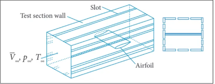
A sketch of the test section is shown in Fig. 3. One wishes to investigate, numerically and experimentally, the low in the Figure 1. Test section of the PTT showing the slotted walls.
Figure 2. Transonic wind tunnel sketch showing the system of forced extraction and reentry laps.
Plenum chamber
Plenum chamber evacuation
Test section
region between the airfoil and the walls of the test section of the tunnel. With the numerical simulation, one can study the low about the airfoil, especially in the form of the pressure distributions on the upper and lower surface of the body. Besides, it is also possible to investigate the low that happens at the slots. Experimentally, the pressure distribution upon the airfoil will be assessed.
where:
x: Cartesian coordinate along the central horizontal axis of symmetry of the tunnel;
y: Cartesian coordinate normal to x and contained in the vertical symmetry plane;
p: static pressure; ρ: density of the luid;
f [s/d]: characteristic tunnel parameter; s stands for the slot width;
d: distance between slots;
ϕ: potential of the velocity perturbations; ∞: free-stream conditions.
As put by Goethert, this equation defines the pressure build-up which occurs in the non-uniform low region near the sloted wall. From these studies, we learn that, if the ratio of open to closed areas at the wall is correctly chosen, the static pressure on the plenum side of the slot is equal to the free-stream value, that is,
Figure 3. Sketch of the PTT’s test section showing the installed NACA 0012. The smaller sketch at the right shows the position of the slots and the front shoulder of the airfoil.
THE NUMERICAL STRATEGY
The Code
he mathematical model is represented by Euler equations, written in generalized coordinates and conservation-law form. By “Euler equations” we recognize the collection of the continuity, momentum, energy, and any constitutive equation necessary to represent the medium. he medium is air, considered as an isotro-pic and Newtonian luid and as a thermally and calorically perfect gas. he numerical algorithm follows closely the main lines of the inite-diference, diagonal scheme due to Pulliam and Chaussee (1981), complemented by a non-linear, spectral-radius-based artiicial dissipation strategy due to Pulliam (1986). he interested reader can ind most of the details of the code, including verii-cation and validation, in Falcão Filho and Ortega (2007, 2008).
Boundary Conditions
he overall treatment of boundary conditions is standard and can be found in most treatises on numerical methods (Hirsch, 2007). he only aspect that deserves special attention here are the slots. Goethert (2007), in chapter 5 of his book, has derived a very ine and consistent analysis of tunnels with slots. One of the points that he treats thoroughly is the one related to the disturbances generated by the slots. With the help of the linearized theory (Liepmann and Roshko, 1956), he gets at the equation:
Test section wall
Airfoil Slot
V∞, р∞, T∞
p = f [s/d] dϕxy ρ∞ V∞ + p∞ (1)
The area ratio referred in the case of the PTT can be considered as correctly chosen, taken into account that the conceptual design of the tunnel was developed by the American firm Sverdrup Technology Inc
®
(Sverdrup Tecnology, Inc, 1989). Under these circumstances, we have adopted Eq. (2) as the basic information at the plane of the slot.But enforcing boundary conditions at the slots is a bit more involved. And this is simply because, along the slot, sometimes the mass might move from the test section to the plenum chamber, and so the plane of the slot can be treated as an exit plane; or, otherwise, if the mass moves from the plenum to the test section, then the slot must be treated as an inlet plane. In order to decide what to do, a lag was introduced at the slot subroutine. he lag is based on the direction of the velocity component normal to the plane of the slot. he velocity component is the one calculated in the last iteration. If this component points to the plenum, the former scenario is the one to be enforced, whilst, if the component points to the test section, the latter scenario is the one which is valid. At the start of the calculation, the plane of the slot was considered as an exit plane.
Another situation that deserves attention is related to the passage of information between blocks (see next subsection). At the meeting of the upper and lower grids (interface between an upper and a lower block), the boundary points are coincident
and, because those are frontier points, they need boundary conditions. Figure 4 illustrates the point. In this instance, a linear interpolation was applied. For η lines, that is, grid lines for constant η, a linear approach was assumed and virtual points 5 and 6 were positioned. Ater that and by simple arithmetic mean, the value of properties at point 7 is obtained. In fact, point 7 is also the result of linear interpolation.
Figure 4. Scheme for the passage of information at the frontier of grids belonging to two different blocks.
The Grid
he position of the foil is the following. For an angle of attack equal to zero, the symmetry plane of the airfoil coincides with the symmetry horizontal plane of the calculation domain (Fig. 3). In this position, the distance of the leading edge to the inlet plane is equal to 0.5585 m. he chord length is 83 mm. For angles of attack diferent from zero, the axis of rotation is a ixed horizontal span axis passing by the mid-chord point. he model spans the whole width of the tunnel and the span axis is normal to the vertical walls.
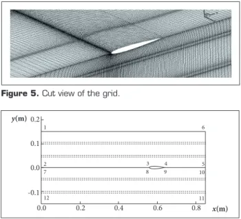
he grid is structured and divided in blocks. Figure 5 shows a cut of the grid with a detail of the airfoil. Information is passed from one block to the other in a natural way by means of a simple strategy: the blocks are treated in sequence, and the neighboring plane of a block which has been already calculated furnishes the adequate boundary conditions for the block that comes next (Fig. 6). his igure shows the division by blocks as seen at a longitudinal plane normal to the airfoil span axis. Figure 7 shows a cut of the overall grid with the airfoil and the clustering of nodes along the slots. he grids for the blocks that do not contain the airfoil surfaces are deined algebraically, whereas the grids for the blocks that do contain the airfoil surfaces are obtained by means of elliptic diferential equation solutions. Figure 8 shows a detail of the grid in the region where the airfoil cuts the loor or the ceiling planes of the test section. Around the airfoil and along the slots, the nodes are clustered, and this is done by means of the many resources ofered by the elliptic grid generator. See also Fig. 9, with the detail of the upper surface of the airfoil. For further details, see Falcão Filho and Ortega (2008).
Figure 8. Details of nodes clustering at the plane of the loor (or ceiling).
y (m)
-2.00E-04
5.580E-01 5.582E-01 5.584E-01 5.586E-01 -1.00E-04
0.00E+00 1.00E-04
Stagnation point Leading edge 2.00E-04
x (m)
1 5 2
7
3 6 4
Figure 5. Cut view of the grid.
Figure 7. Cut view of the grid showing the airfoil and the clustering of nodes along the slots.
Figure 6. Division of the calculation domain in blocks: (1 - 2 - 3 - 4 - 5 - 6) and (7 - 8 - 9 - 10 - 11 - 12).
Figure 9. Detail of the grid along the longitudinal symmetrical plane and including the upper surface of the airfoil.
6
3 4 5
8 9 10
11 12
2 7 1
0.2
0.2 0.4 0.6 0.8
0.1
0.0
0.0 -0.1
x(m)
y(m)
} Slot
} Slot -0.030
0.540 0.560 0.580 0.600 0.620 0.640
-0.010 0.010 0.030
x(m)
RESULTS AND DISCUSSION
Table 1 shows the cases that were investigated. In order to spare space a selection of cases, the most representative ones will be discussed. As called attention, in this article, we shall concentrate on the numerical results by confronting solid wall against perforated wall simulations. In order to enrich the presentation and bring trustworthiness to the data, comparison with experimental results will also be provided.
lower when compared to the ventilated wall solution. his is a result of the over-acceleration of the low for the former case. Second, the data for the slotted wall case compare well with the literature’s experimental values (Harris, 1981, for a Reynolds number equal to 3 × 10⁶).
he closeness of the experimental values and the slotted wall solution is indicative that the numerical code is doing well in the simulation of the low in the slots. In order to illustrate this important result, we plotted values in Fig. 13 to show the inclination of the velocity vector along one of the upper central slots. In the igure, we have also drawn the real form of the slot, together with the position of the airfoil’s edges, which are marked by dashed lines. At the inlet section, the inclination (θ),
Figure 12. Pressure distributions along the chord of the airfoil.
Figure 11. Velocity vectors in the stagnation region for case 1 (slotted walls).
Figure 10. Number of Mach levels around the airfoil for case 1 (slotted walls).
Case Mach number (M∞) Angle of attack (α)
1 0.6 0°
2 0.6 2°
3 0.6 4°
4 0.6 6°
5 0.6 8°
6 0.7 0°
7 0.7 2°
8 0.7 4°
9 0.8 0°
10 0.8 2°
Table 1. Main characteristics of the cases investigated.
NUMERICAL RESULTS
Case 1: Mach Number = 0.6; Angle of Attack = 0°
Results for solid and slotted walls will be compared and discussed. Figure 10 is representative of the Mach number map in a zoomed area around the airfoil. he symmetry of values in relation to the symmetry plane is outstanding. Attention should be called to the fact that the solid black line in the igure represents the frontier between two of the individual blocks that form the entire grid. We call attention to this point in order to stress the fact that the boundary conditions, in general, and the passage of information between blocks, in particular, are working well. In order to better ix the point, we show Fig. 11. he velocity ield is symmetric and the speed is zero at the stagnation point.
he pressure distributions in terms of
are plotted in Fig. 12. As the reader can observe, the diferences between the simulated values are small in this case — maximum 2.06%. Note that here one has M∞= 0.6 and α = 0°, a situation far from the sonic low. Two aspects are worth noting. First, the pressure for the solid wall solution along the airfoil is systematically
cp = 2(p − p∞)/ρ∞V2
∞ (3)
0.05
0.00
0.50 0.55 0.60 0.65 0.70 0.75
-0.05
y(m)
x(m)
Stagnation point
0.556 -0.002
-0.001 0.000 0.001
y(m)
x(m)
0.002
0.558 0.560 0.562
Experiment (Harris, 1981) PTT-PSP
Slotted walls Solid walls
1.2
0.0 0.2 0.4 0.6 0.8 1.0 0.8
0.4 0.0 -0.4
Cp
relative to a horizontal plane, is zero, and the low is parallel to the plane of the slot. At irst, it was thought that, for this case, M∞ = 0.6 and α = 0°, a mild case, there would be not much “mass transit” through the slots. But, as can be observed in the igure, this is not the case. he maximum value of θ is -2.7°. Another aspect that deserves attention is the fact that mass enters the plenum almost immediately by the action of the high pressure at the stagnation region of the airfoil. he suction at the upper surface of the foil brings the mass back to the test section, and the process of entering begins at a point in the slot situated at 0.20c ahead of the leading edge (this is only the horizontal distance). he maximum inclination of the velocity vector during the re-entering process is -2.7° at a point in the slot whose horizontal distance to the leading edge is about 0.16c. Ater this position, the velocity vector starts to recover its initial horizontal direction at the slot. here is a region of a mild direction oscillation ahead of the airfoil, and this is marked in the igure by a closed line. his is simply the inluence of the special geometrical form of the slot.
Case 3: Mach Number = 0.6; Angle of Attack = 4°
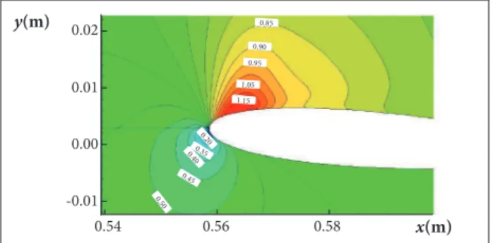
For a free-stream Mach number, M∞ = 0.6, this case is a sort of “dividing-line” case, because it separates tendencies. For the first time, we have the appearance of a typical transonic/supersonic scenario at the upper surface of the airfoil. But this is only for the solid wall coniguration (Fig. 15). In order to stress the point, we present Fig. 16, where the supersonic bubble is perfectly deined. he shock therefore is a consequence. The same case, although run with the slots opened, prevents the appearance of the supersonic bubble and there is only a sonic point located at the leading edge. In this case, therefore, there is no formation of the shock wave. In order to deinitely ix the point, we present Fig. 17. The typical transonic pressure profile is present with the shock for the case of the solid walls. It should be noted that, in this case, the maximum difference between the two upper surface distributions is really great.
Case 4: Mach Number = 0.6; Angle of Attack = 6°
Case 4 is very important. It marks the frontier between cases with and without shocks (for the overall conditions of this experiment, naturally). Figure 18 shows the reason why. Now, the shock appears even with the slots opened. To illustrate the Figure 13. Inclination of the velocity vector relative to a
horizontal plane, θ, along the upper slot (case 1).
Figure 14. Inclination of the velocity vector relative to a horizontal plane, θ, along the upper slot (case 2).
Case 2: Mach Number = 0.6; Angle of Attack = 2°
This case is also completely subsonic. Because the angle of attack is different from zero, there is an unbalance between the pressure distribution on the upper and lower surfaces. The pressure distributions on the surfaces of the airfoil take the classical form. What is interesting here is to appreciate the strengthening of the mass flow passing through the slots following the increase of the angle of attack. Figure 14 shows all those aspects. The largest incli-nation now is -7.5°, a much stronger effect when compared to the last case. Another point to be stressed here is the difficulty of the flow in the slot to realign to the horizon-tal direction after the airfoil station, indicating a possible downwash effect.
1,38 c
c
-8.0
0 0.1 0.2 0.3 0.4 0.5 0.6 0.7 0.8 -6.0
-4.0 -2.0 0.0 2.0
x(m)
θ
1,99 c 0,84 c
c
-8.0
0 0.1 0.2 0.3 0.4 0.5 0.6 0.7 0.8 -6.0
-4.0 -2.0 0.0 2.0
x(m)
θ
Figure 15. Levels of Mach number for the NACA 0012 (case 3; solid wall).
0.05
0.50 0.55 x(m)
y(m)
0.60 0.65 0.70 -0.05
0.00
0.55
0.55
0.65
0.50 0.70
0.75
0.80 0.85 0.90
0.401.15
0.60
case, we have plotted in the igure the experimental results of our measurements. Our calculation and the measurements of Harris (1981) do not detect the shock. In our instance, the reason is related to the mathematical model that we have used, that is, the Euler equations. In Harris case, the boundary layer was turbulent and therefore it had “suicient strength” in order not to be detached by the mild pressure gradient introduced by the shock. But, interestingly, our measurements detected the recirculation bubble and this is indicated by the sudden rise in pressure close to the airfoil leading edge. he reason behind this apparently strange behavior is that, in practice, the boundary layer is laminar due to the fact that the Reynolds number is quite low at the PTT. In Gofert et al. (2014), the reader can ind a detailed analysis of this point.
Lift Analysis for Cases 1, 2, 3, and 4
A very instructive study is the one relating cl, the lift coeicient, to the airfoil’s angle of attack. Especially, for low values of α, the relationship is basically linear. In Fig. 19, we have plotted cl versus α for cases 1, 2, 3, and 4, as well as for solid and ventilated walls. For comparison purposes, the experimental values of Harris (1981), for Rc= 3 × 10⁶, is also
shown (Rc is the Reynolds number based on the chord c of the foil). For this range of angles of attack, the correlations between the experimental and ventilated walls are basically linear. he maximum diference is ∆cl = 0.065 for α = 6°. he solid wall distribution is not exactly linear when one considers the complete range 0° – 6°, and for α = 4°, the diference in cl relative to the experimental data is 54.5%.
McCroskey, in his work of 1987, reports, from several sources, values of clα = dcl /dα as function of the Mach number. his is one of the most important of the so called “aerodynamic coeicients”, which are instrumental in light mechanics. For M∞ = 0.6, the values given by McCroskey fall in the range of 0.110 – 0.140. In the present simulations, we have obtained 0.122 and 0.169, respectively for slotted and solid walls. It is evident that only the solution for the ventilated wall is a good value.
Figure 16. Zoom of Mach number ield at the leading edge (case 3; solid wall).
Figure 18. Pressure distribution along the chord of the airfoil (case 4).
Figure 19. Lift coeficient versus angle of attack for cases 1, 2, 3, and 4.
Figure 17. Pressure distribution along the chord of the airfoil (case 3).
Case 3: Three-Dimensional Effects
In spite of the mathematical model being here represented by the Euler equations — and therefore boundary layers and shear layers are not present, besides the fact that the airfoil is “two-dimensional”, in other words, the transversal sections along the span are always the same and the span axis is normal to the tunnel walls —, there will appear three-dimensional efects in the ield. And this is mainly due to a “side-efect” of the ventilating action. We shall focus the discussion on this point. To begin, it is necessary to present parts of the low ield along certain speciic surfaces. In Figs. 20 and 21, the plane that appears before and ater the wing (marked with the dashed lines) corresponds to
0.02
0.01
0.00
0.54 0.56 0.58
-0.01
x(m) 0.50
0.45 0.400.35
0.20 1.15
1.05 0.95
0.90 0.85
y(m)
-2.2
-1.4
-0.6
0.2
1.0
0.0 0.2 0.4 0.6 0.8 1.0
Cp
x/c
Experimental (Harris, 1981) PTT-PSP
Slotted walls Solid walls
Experiment (Harris, 1981) PTT-PSI
PTT-PSP CFD
PSI: classical static-pressure tap method.
x/c Cp
-1.2 -2.0
-0.4
0.4
1.2
0.0 0.2 0.4 0.6 0.8 1.0
CFD – Solid walls Experiment (Harris, 1981) CFD – Slotted walls
cL
α
-0.2
0.0 2.0 4.0 6.0
the test section central horizontal plane. In the region between the dashed lines, what appears is the upper surface of the airfoil. Along the complete surface, we plot the pressure distribution. In the case of the solid walls (Fig. 20), the level lines of pressure along the span are perfect straight lines, with the exception of a small region close to the wall and near the leading edge. his might be due to the presence of the shock near the tunnel wall.
In the case of the pressure distribution upon the same surface, but with ventilation in action (Fig. 21), the perturbations on the level lines, in spite of still being small, are discernible and present along all the span and chord directions. As in the case of the solid walls, the deviation is greater in regions close to the wall. But here, because we do not have shocks, the cause for the deviation to grow near the walls must be of a diferent nature. To understand the actual nature of the low, we will rely on a vertical surface as shown in Fig. 22. his surface is constituted by a vertical plane that starts at the leading edge and cuts the grid upper semi-block.
Figures 23 and 24 illustrate and explain the three-dimen-sional efects, which, in this situation, are induced by the action of the ventilation through the slotted walls. In Fig. 23, the simulation is considering the walls as solid, whereas in Fig. 24, the ventilation is working. What happens is that ventilation introduces a cross-low component of velocity in the tunnel stream. his is even better illustrated in Figs. 25, 26, and 27, where the cross-low jets are shown. Observe that, at the lateral
slots, there is mass low whose transverse component Vzmay reach about 8% of V∞. he mass induction entering the test section is a result of the pressure diference between the slot and the upper surface of the airfoil. herefore, when mass crosses the lateral slots, the static pressure will rise slightly in the region next to the wall and next to the airfoil.
Figure 20. Levels of pressure for the NACA 0012 at the test section central horizontal plane (case 3; solid walls).
Figure 24. Levels of pressure at the test section central vertical plane (case 3; ventilated walls).
Figure 25. Transversal plane ventilated lux through the slots (case 3; ventilated walls).
Figure 23. Levels of pressure at the test section central vertical plane (case 3; solid walls).
Figure 22. Positioning of the transversal plane that will be used in the plotting of results.
Figure 21. Levels of pressure for the NACA 0012 at the test section central horizontal plane (case 3; ventilated walls).
x (m) z (m)
0.00 0.10
0.40 0.50 0.60 0.70 0.80 0.20
0.30
1.00
1.00
0.70
0.55 0.85
0.75 0.95
0.80
1.00
0.90 1.05
1.05
1.10
x (m)
z (m)
0.05 0.10
0.40 0.50 0.60 0.70 0.80 0.15
0.20 0.25
1.00 0.70 0.800.850.90 0.95 1.00 1.05 1.00
z (m)
y (m)
0.05
0.00 0.05 0.10 0.15 0.20 0.25 0.10
0.15
0.970
0.950 0.940
0.930 0.920 0.910
0.960
0.960 0.960
0.980
0.980 0.980
0.980
0.980
z (m)
y (m)
0.06
0.02
0.00 0.05 0.10 0.15 0.20 0.25 0.10
0.14
z (m)
y (m)
0.02 0.06
0.00 0.05 0.10 0.15 0.20 0.25 0.10
0.14
1.00
0.70 0.60 0.85
0.75 0.95
0.80 0.90
Transversal plane
Cases 6, 7, and 8: Mach Number = 0.7
As a matter of illustration of all these cases, we present only the distributions of pressure for the case M∞ = 0.7 and α = 2° in Fig. 28. he results here are very similar to the low characteristics for M∞ = 0.3, including the tendencies of the cl and the pitching lit derivative, clα = dcl /dα. herefore, there is no reason to discuss these aspects again.
In the literature, there is a scattering of values for the position of the shock wave relative to the chord of the airfoil. A simple look in McCroskey (1987) will conirm this fact. he reasons are varied: (i) diferent tunnels: solid walls, perforated walls, slotted walls; (ii) diferent model blocking ratios; (iii) diferent values of the Reynolds numbers, one of the most important inluences. According to literature data collected by McCroskey, the position may vary in the range of 35 to 55% of the aerodynamic chord with a mean value of 46 ± 2%. According to Fig. 29, our numerical simulation with solid walls, the position of the shock is well beyond 50% of the chord. For the ventilated simulation, the position is given by 45 ± 2%. Besides the large deviation in the position of the wave, the intensity of the jump is much more efective when the walls are solid. As we have already called attention before, the question here is related to the relief efect that is present when the walls are perforated. In a tunnel with solid walls, the mass rate is maintained downstream, the mean speed at the airfoil region is larger — when compared to the same tunnel with ventilated walls —, and the result is a stronger shock positioned nearer to the trailing edge.
McCroskey cites two main factors that may deviate the position of the wave: wall interference and errors associated to the Mach number. In terms of wall interference, there is no doubt that the main factor is the boundary layer formation along the walls of the tunnel. he presence of the boundary layer has many consequences. he irst is that it diminishes Figure 28. Pressure distributions along the chord of the
airfoil (M∞ = 0.7 and α = 2°).
Figure 27. Velocity vectors at the transversal plane of Fig. 25 in a region next to the slot (case 3; ventilated walls). This map corresponds to the lower slot in Fig. 25.
Figure 30. Pressure levels about the airfoil (M∞ = 0.8 and
α = 0°; slotted walls).
Figure 26. Velocity vectors at the transversal plane of Fig. 25 in a region next to the slot (case 3; ventilated walls). This map corresponds to the upper slot in Fig. 25.
Figure 29. Pressure levels about the airfoil (M∞ = 0.8 and α= 0°; solid walls).
-1.2
-0.4
0.4
1.2
0.0 0.2 0.4 0.6 0.8 1.0
Cp
x/c Experiment (Harris, 1981) PTT-PSP
Slotted walls Solid walls
0.035
0.030
-0.005 0.000 0.005 0.010 0.025
y (m)
x (m)
1.15 1.00
1.00
1.10 0.95 0.90
0.85
0.75 0.65
1.20 1.10 1.05
y (m)
x (m)
0.05
0.50 0.55 0.60 0.65 0.70 0.75 0.00
-0.05
0.80 1.05
0.095
0.090
-0.005 0.000 0.005 0.010 0.085
y (m)
x (m)
1.15 1.00
1.00 0.95
0.90 0.85 0.80
0.75 0.70
0.65 0.55 1.10 1.10
1.05
1.05
y (m)
x (m) 0.05
0.50 0.55 0.60 0.65 0.70 0.75
0.00
-0.05
Cases 9 and 10: Mach Number = 0.8. Position of the Shock Wave
Slot Direction of low Total mass lux per slot
1 in + 0.0199
2 out - 0.0088
3 out - 0.0094
4 out - 0.0088
5 out - 0.0084
6 in + 0.0255
Total in + 0.0100
Table 2. Total mass lux that crosses the slots of the upper grid half block.
In: mass entering the test section; out: mass exiting the test section. the efective transversal passage area for the low. Besides, the
performance of the wall ventilation is diminished, and, inally, one must be aware that the boundary layer is a irst order factor in the induction of three-dimensionality of the low in the tunnel.
Cases 9 and 10: Three-Dimensional Effects
hree cp distributions were drawn for case study 9, M∞ = 0.8 and α = 0°. he positions along the span are: (i) z = 0.0 mm, that is, at the wall; (ii) z = 62.5 mm, that is, one fourth of the total span length from the wall; (iii) and z = 125.0 mm, that is, at the center span position. he results can be seen at Fig. 31. he reader can observe the discrepancies in the data and the rather strong inluence of the wall upon the pressure distributions on the airfoil’s surface. his is the direct efect of the low at the slot upon the low pressure region at the upper surface of the airfoil. As can be observed, in the position z = 0.0 mm the mass lux coming from the slots gives rise to a blocking efect and augments the static pressure on the foil’s upper surface. Consequently, the main low is decelerated and the shock wave looses intensity. As the section “moves” away from the wall, and also from the slot exit, the mass coming from the slot redistributes to a larger portion of the main low, and the inluence upon the pressure distributions diminishes accordingly.
Global Slot Effects for Case 9
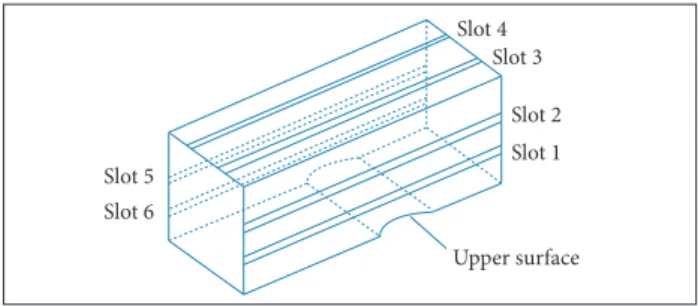
In this section, we shall present some total results due to the action of all the slots. To this end, we start with Fig. 31, in which we diferentiate the slots by numbers. Figure 31 corresponds to the upper semi-block of the dominion of flow. Part of the inferior surface is formed by the upper surface of the airfoil. Now, let us fix attention on Fig. 32. At slot 1, which is located 27.8 mm from the base symmetrical plane (y = 0), mass is being expelled from the test section until the leading edge
of the foil. But after this point, due to the under pressure on top of the body, mass is induced to enter the test section, and, inclusively, the angle of the velocity vector falls to -26°. The balance is 0.020 kg/s of mass exiting the test section for the whole slot 1. For the slot 2, located 87.8 mm from the base plane, the total of mass leaving the test section is 0.009 kg/s (the total mass flux that crosses the slot is obtained by numerical integration, after the solution is converged).
Table 2 shows the average directions and the total mass lux for each slot. At slots 1 and 6, which are positioned closer to the model, the total mass lux has the tendency, in mean terms, of entering the test section. For the other slots, 2, 3, 4, and 5, the tendency of the balance of mass is to leave the test section. But because the mass lux through slots 1 and 6 is greater, the total balance, taking into account all slots, is entering the test section on a basis of 0.01 kg/s.
Figure 31. Pressure distributions for different positions (M∞ = 0.8 and α = 0°).
z = 0,0 mm z = 62,5 mm z = 125,0 mm PTT-PSI PTT-PSP
PSI: classical static-pressure tap method. 1.2
0.0 0.4 0.8
0.4 -0.4 -1.2
x/c Cp
Figure 32. Identiication of the slots with numbers.
Slot 5 Slot 6
Slot 1 Slot 2 Slot 3 Slot 4
Upper surface
CONCLUSIONS
he investigation of an airfoil in a TWT, both numerical and experimental, is not an easy task. In the numerical case, for example, the dominion of low has to be three-dimensional and the slots have to be taken into account. We believe, or, at least, we hope, that we have done a good job. he adoption of the Euler equations was a key-decision at this point of the project. Such a simpler mathematical model allowed the probing of many of the most important aspects presented by the problem, without getting too much involved with the ever cumbersome number of points when the Navier-Stokes equations are called upon. he level of stifness brought to the problem by the latter equations is notable — see, for example, Falcão Filho and Ortega (2008).
Probably, the most important problem of a solid wall wind tunnel working at the transonic range is the choking efect. We have shown, without a doubt, the action of the ventilation in this respect. Figure 17 conirms this assertion. he existence of the slots, that provides the ventilation of the test section, simply eliminated the existence of a virtual shock wave, which, evidently, would not appear at free-stream conditions. Another inding that deserves attention is the distribution of mass lux along a slot. When the tunnel stream enters the test section, there is always an outlow of mass, a consequence of a certain blockage exerted by the high-pressure stagnation region along the entire span. When suction prevails, i.e. the pressure is lower when compared to the plenum, downstream to the leading edge and at the upper surface of the foil, mass is “brought back”. hese efects are directly related to V∞ and the angle of attack, which is conirmed by Figs. 13, 14 and 34.
Figure 33. Values of the total mass lux that crosses all slots, for several values of the free-stream Mach number and the NACA-0012.
Figure 34. Direction of the low in the lateral slots for case 9.
Angle of attack
M
ass fl
o
w r
at
e thr
o
ug
h s
lo
ts
(kg/s)
0.00
0.00 2.00 4.00 6.00
0.04 0.08 0.12
Mach 0,6 Mach 0,7 Mach 0,8
Slot 1 Slot 2 NACA 0012 limits
β
x(m)
-30.0
0 0.2 0.4 0.6 0.8
-20.0 -10.0 0.0 10.0
A very important result is related to the lift curve slope, clα. For M∞ = 0.8, we obtained the value of 0.122 for this parameter with the slots opened. This value falls well inside the range of 0.110 – 0.140 given by McCroskey (1987). On the other hand, the value that we have obtained with the slots closed is well outside this range. Another successful verification is related to the position of the shock wave relative to the chord. For M∞ = 0.8, α = 0.0 and slots opened, we have obtained a value of 45 ± 2%, while McCroskey gives a mean value of 46 ± 2%.
On the other hand, ventilation has a side efect. It induces some three-dimensionality in the tunnel stream. In this work, we calculated the balance of mass low crossing the slots. But the balance per se does not provide a clue of how to handle this problem. Considering the assortment of good results that we have obtained, it seems that the influence of this side efect is very small. But this point must be investigated further in order to place a deinite word. It is one of our next aims to introduce the efects of turbulence in this problem. We already have some experience in this matter related to the process of injection in TWTs — see Falcão Filho and Ortega (2007, 2008). Ater these investigations, maybe some light will be shed upon this problem.
ACKNOWLEDGEMENTS
REFERENCES
Abbott, I.H. and von Doenhoff, A.E., 1959, Theory of Wing Sections, Dover Publications, Inc., New York, USA.
Falcão Filho, J.B.P. and Ortega, M.A., 2007, Numerical Study of the Injection Process in a Transonic Wind Tunnel. Part I: the Design Point, Journal of Fluids Engineering, Vol. 129, No. 6, pp. 682-694. doi: 10.1115/1.2734236
Falcão Filho, J.B.P. and Ortega, M.A., 2008, Numerical Study of the Injection Process in a Transonic Wind Tunnel: the Numerical Details, Computers Fluids, Vol. 37, No. 10, pp. 1276-1308. doi: 10.1016/j. compluid.2007.10.015
Goethert, B.H., 2007, Transonic Wind Tunnel Testing, Dover Publications, Inc., New York, USA.
Goffert, B., Ortega, M.A. and Falcão Filho, J.B.P., 2014, Wall Ventilation Effects upon the Flow about an Airfoil in a Transonic Wind Tunnel, Experimental Techniques, doi: 10.1111/ext.12085
Harris, C.D., 1981, Two-Dimensional Aerodynamic Characteristics of the NACA 0012 Airfoil in the Langley 8-Foot Transonic Pressure Tunnel. NASA Technical Memorandum 81927.
Hirsch, C., 2007, Numerical Computation of Internal and External Flows, Butterworth Hannemann, Burlington, USA.
Ladson, C.L., 1957, Two-Dimensional Airfoil Characteristics of Four NACA 6A-Series Airfoils at Transonic Mach Numbers up to 1.25, NACA Research Memorandum RM-L57F05.
Liepmann, H.W. and Roshko, A., 1957, “Elements of Gasdynamics”, John Wiley and Sons, Inc., New York, USA.
McCroskey, W.J., 1987, A Critical Assessment of Wind Tunnel Results for the NACA 0012 Airfoil, NASA Technical Memorandum 100019.
Noonan, K.W. and Bingham, G.J., 1977, Two-Dimensional Aerodynamic Characteristics of Several Rotorcraft Airfoils at Mach Number from 0.35 to 0.90, NASA Technical Memorandum X-73990.
Pulliam, T.H., 1986, Artiicial Dissipation Models for the Euler Equations, AIAA Journal, Vol. 24, No. 12, pp. 1931-1940.
Pulliam, T.H. and Chaussee, D.S., 1981, A Diagonal Form of an Implicit Approximate-Factorization Algorithm, Journal of Computational Physics, Vol. 39, No. 2, pp. 347-363. doi: 10.1016/0021-9991(81)90156-X
Scheitle, H. and Wagner, S., 1991, Inluences of Wind Tunnel Parameters on Airfoil Characteristics at High Subsonic Speeds, Experiments in Fluids, Vol. 12, No. 1-2, pp. 90-96. doi: 10.1007/BF00226571