Faculdade de Engenharia da Universidade do Porto
and
University of Maryland, Baltimore County
Master in Mechanical Engineering
Thermal Energy
Project
Computer Simulation of an
Internal Combustion Engine
Supervisor in UMBC: Dr. Christian von Kerczek
Advisor in FEUP: Prof. Eduardo Oliveira Fernandes
Exchange Advisor: Dr. L.D. Timmie Topoleski
Acknowledgments
I would like to express my gratitude to Dr. Christian von Kerczek
for his dedication and devotion for this project.
I also would like to thank my parents for this life time opportunity,
“Obrigado!”
Contents
Commonly used symbols, subscripts, and abbreviations 5
Abstract 8
Objectives 9
Introduction 10
Chapter 1- Internal Combustion Engine 12
1.1.The Basic ICE Mechanism 12
1.2.The Equations of State of the Working Gases 16
1.3.Thermodynamics and Mathematical Model of the Engine 17
Chapter 2 - Power Cycle 19
2.1.Introduction 19
2.2.Compression stage 20
2.2.1 Thermodynamic Model of the compression stage 20
2.2.2 Heat transfer 21
2.3.Combustion stage 24
2.3.1 Combustion modeling 24
2.3.2 Turbulence characteristics 31
2.3.3 Heat Transfer 33
2.4.Completely burned gas expansion 34
2.4.1 Thermodynamic model of the expansion stage 35
2.4.2 Heat Transfer 35
Chapter 3 – Gas exchange cycle 37
3.1.Valve action 37
3.1.1 Geometry 37
3.1.2 Isentropic flow thought an orifice 39
3.2. Exhaust stage 40
3.2.1 Thermodynamics Model of the Exhaust stage 41
3.2.2 Heat transfer 41
2.3. Intake stage 42
3.3.1 Thermodynamics Model of the Intake stage 42
3.3.2 Heat transfer 43
CycleComQC Inputs 44
Conclusive remarks 59
Bibliography 60
Appendixes 61
A Mathematical and thermodynamic manipulations 61
B Definitions 72
Commonly used symbols, subscripts, and abbreviations
1. Symbols
a Crank radius
Ac Clearance volume
Af Effective flow area
Ap Port area
Av Valve cross sectional area
Aw Exposed total cylinder area
bo Cylinder bore
co Sound speed
Cf Flow coefficient
Cp Specific heat at constant pressure
Cv Specific heat at constant volume
d Diameter
D Diameter
h Specific enthalpy
h Height
hg Heat transfer coefficient
k Turbulent kinetic energy
l Connecting rod length
Valve lift
m Mass
mr Residual mass
m
Mass flow rate respective to time
m
Mass flow rate respective to angleN Crankshaft rotational speed
P Pressure
Power
Q
Heat transfer rate respective to time
Q
Heat transfer rate respective to angler Radius
rc Compression ratio
s Stroke
T Temperature
u Specific internal energy
U Internal energy V Velocity Speed Cylinder volume Vc Clearance volume Vd Displacement volume W Work transfer x Mass fraction
xr Residual mass fraction
θ Crank angle ρ Density ωs Angular velocity
2. Subscripts
b Burned gas cr Crevice e Exhaust f fuel i Intake L Laminar u Unburned v valve w wall o Reference value Stagnation value3. Notation
~ Value per second
^ Value per angle
4. Abbreviations
BC Bottom-center crank position
ICE Internal Combustion Engine
Abstract
My end course project was performed in the exchange program between Faculdade de Engenharia da Universidade do Porto (FEUP) and the University of Maryland, Baltimore County (UMBC).
The project was proposed by Dr. Christian von Kerczek (CVK) who developed a thermodynamic engine model for which a computer program had been written for its implementation.
The computer simulation was developed and implemented numerically by way of a “Scilab”. However, heat transfer, Q (Q=0), was left out which results somewhat artificially in an "adiabatic engine". Also the combustion model used was based on a somewhat simple formulation. It was assumed that burned and unburned gases were homogeneously mixed and burning rate was a constant. Based on CVK work, my work has added heat transfer and a two zone combustion model that separates the action of the burned and unburned gases during the combustion. The boundary of these zones was then determined by a turbulence flame speed model.
In both of these cases, there exist well developed empirical models, and the main objective of my work was to understand and adjust these models and implement them within the theoretical model and the computer program developed by CVK.
This work contains a complete description of the theoretical framework employed by CVK as well as the modifications and implementation of heat transfer and combustion model by me.
The result of my project is a computer simulation which may be used to obtain some fairly good estimates of engine performance. These estimates are most useful for understanding basic engine performance as well as assessing modifications as regards valve sizing, spark advance and various fuels. A particularly useful application is to do a compressor/turbine engine matching for turbocharging.
Objectives
The main propose of my work:
● Complete the program with the heat transfer model and insert the correct modifications to
perform a simulation of a non adiabatic engine;
● Add a new combustion model, replacing the existing one used in the initial program. The
new combustion model would take into account the turbulence in the cylinder and would then allow the variation of burn duration (which is fixed in the simple model used) to vary with engine speed.
Despite this, I also had to understand the existing computer simulation implemented by CVK and the theoretical concepts behind it.
Introduction
This report presents the Thermodynamics theory describing the main physical phenomena occurring inside a spark ignition four stroke (4S) internal combustion engine (ICE) while it is running at steady speed (constant revolutions per minute, rpm). The mathematical form of the Thermodynamic theory is developed and implemented numerically by way of a “Scilab” computer program. The result is an ICE computer simulation. This computer simulation may be used to obtain some fairly good estimates of engine performance in which the main effects of compression ratio, sparks timing, some aspects of valve timing, valve sizing, and fuel types, over a range of engine speeds.
Of course not every detail of ICE performance can be accounted for, but depending on the physical details incorporated and their relative importance, many of the most important performance characteristics can be determined to a reasonable degree of accuracy. This report does not deal with any structural or mechanical aspects of an ICE beyond those of the basic geometric features relevant to the containment and external manifestations of the Thermodynamics processes occurring in the engine. These thermodynamic processes are idealized to a certain degree in order to reduce the complexity at this stage of development of the engine simulation.
The simulation is based on the standard configuration of a reciprocating piston in a cylinder closed at one end, the cylinder 'head'. The piston is connected to a crank by way of a connecting rod that protrudes out the opposite open end of the cylinder and connects to a crank. Figure 1 is a schematic diagram of one cylinder of an ICE. The resulting reciprocating motion of the piston imparts a rotation to the crank. This basic slider-crank mechanism (the piston being the slider) transmits power generated by a working fluid, or gas, in the space enclosed by the piston, cylinder and cylinder head, to whatever is connected to crank. The crank is also geared to a camshaft that operates the valves in the cylinder head that periodically open and close to expel or inhale the working gases. Most ICE's have multiple cylinders operating in unison on a common crankshaft. The processes that occur are essentially identical for each cylinder so that the analysis need be done for only one cylinder. The ICE performance is then simply the number of cylinders times the input/output for a single cylinder.
Figure 1 – Four stroke internal combustion engine. [5]
The ICE Thermodynamics analysis is based on the following primary assumptions. All thermodynamics processes are assumed to be internally reversible. The working medium (fuel and air mixtures) is assumed to be an ideal gas with constant specific heats. The equations of state for the burned and unburned media are derived on the basis of equilibrium chemistry. The gas exchange process is based on quasi-steady compressible flow through an orifice.
Further secondary assumptions and idealizations are discussed in the formulation of the thermodynamics model in the next chapters.
Chapter 1- Internal Combustion Engine
1.1.The Basic ICE Mechanism
The piston cylinder-crank mechanism (the slider-crank) is shown schematically in Figure 2. This figure indicates how the up and down motion of the piston turns the crank. The space enclosed by the piston and the cylinder is the main concern here. This is where the latent energy of the fuel-air mixture is released by combustion (oxidized) to produce the sensible energy, which drives the piston. The top of the cylinder enclosure contains an intake and exhaust valve which open and close at appropriate moments of the engine cycle to allow escape of burned gases and ingestion of fresh fuel-air mixture.
Figure 2 - A four-stroke spark ignition cycle. [5]
The basic engine performance cycles are controlled by the crank rotation. The crank rotation in
turn moves the piston up and down, thus varying the volume
V
of the space enclosed by the pistonand cylinder. This varying volume is the primary controlling factor of the sequence of thermodynamic events occurring in the piston-cylinder space. Henceforth this space will be referred to simply as the cylinder.
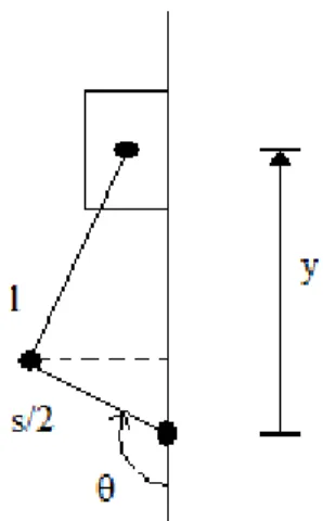
Figure 3 - Sketch of the slider crank model of piston-cylinder geometry
At θ=0 (
2∗n∗π
) the piston is at the bottom-most point in its travel. This point is called bottom center, BC. The cylinder volume V(θ) can be shown, by an analysis of the slider-crank mechanism to be,v =V
m∗
1
r
c
1
2
∗1−
1
r
c∗
1cos R
c−
R
c−sin
2
(1.1)In formula (1.1), Vm is the (maximum) volume in the cylinder at BC,
R
c is the ratio of connectingrod length to
s
, wheres=stroke
, andr
c is the compression ratioV
mV
c, where Vc is the
(minimum) volume of the cylinder at top center (TC) or θ=π
2∗ n−1∗
. Vc is called theclearance volume and
V
d=
V
m−
V
c is the “displacement” volume, the usual measure of engine capacity or, more commonly, engine size.The calculation of the instantaneous volume equation (1.1) is discussed in “Appendix A.1”.
Using Vm as an input variable, some other variables such as the Vc, Vd , bore (bo) and stroke (s)
have to be calculated in order to proceed. It was assumed that the bore was equal to the stroke in order to simplify some equations and to use the minimum ones possible,
V
d=
4
∗
b
2
Vd Vc=rc−1 (1.3)
Vc=
Vm
rc
(1.4)h
c=
4∗V
c∗
bo
(1.5)assuming that the shape of the clearance volume is a cylinder with diameter
bo
and height, hc(Figure 4).
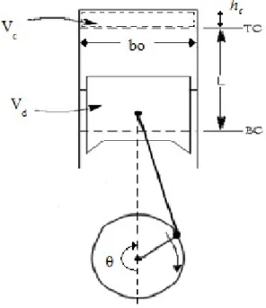
Figure 4 – Basic geometry of the internal combustion engine
The exposed total cylinder area
A
w
is the sum of the cylinder clearance area and the displacement area,A
w=
v−V
cbo /8
A
c (1.7) andA
c=∗
bo∗h
c
2
bo
2 (1.8)The operation of the valves is synchronized to the motion of the piston by way of gear or chain drives from the crankshaft. This is not shown in Figure 2. There will be no need for a description of this mechanism here since it will not be made use of. For the present it is only necessary to describe the valve configuration and actual motion of the valves as a function of the crank angle θ. This will be reserved for the chapter on the gas exchange process in order to keep the exposition simple at this stage. The function, of θ, describing the motion of the valves is given as part of the basic engine specifications utilized in this study. The camshaft and valve actuation mechanism must then be designed to realize this valve motion function. For this the reader is referred to books on engine and mechanism design given in the bibliography.
1.2.The Equations of State of the Working Gases
This gaseous mixture is assumed to be an ideal gas, albeit with different equations of state in the unburned and burned states. The equations of state of the unburned (subscript u) and burned (subscript b) are derived on the basis of combustion equilibrium chemistry and the coefficients of the thermodynamic properties are given in Reference 1. These two thermodynamic laws apply to the gaseous fuel-air mixture in the cylinder. The linearized versions of the equations are used here. For illustrative purpose the fuel used here is CH4 with an equivalence ratio of 1 and whose properties are
very similar to gasoline. During the process of combustion the cylinder contains a mixture of the unburned and burned fuel-air. The mixture is quantified by the burned to total mass ratio
x=
m
bm
,where
m=m
b
m
u . The equations of state for for each of the gases isPV
u=
m
u∗
R
u∗
T
(1.9) andu
u=
Cv
u∗
T hf
u (1.10)PV
b=
m
b∗
R
b∗
T
(1.11) andu
b=
Cv
b∗
T hf
b (1.12)then, if the gases are homogeneously mixed,
PV =m∗ xRb1− x Ru∗T =mRT (1.13) and
U =m∗u=m∗ x∗Cv
b1− x∗Cv
u∗
T x∗hf
b
1−x ∗hf
u (1.14)CVK utilized the homogeneously mixed charge described by equations (1.13) and (1.14), where
dx t
dt
is an empirically determined burning rate.One of the main aims of this study is to implement a more realistic combustion model in which unburned and burned gases remain separated, ie., a “two zone” model.
1.3.Thermodynamics and Mathematical Model of the Engine
The engine operates in a two-cycle (4 stroke) mode. Each cycle consists of a complete rotation, through an angle of 2π, of the crank. The first cycle is called the power cycle in which both valves are closed and the power of the engine is produced. This cycle consists of the compressions stroke roughly from θ=0 to θ=π, in which the fuel-air mixture in the cylinder is compressed, followed by the expansion stroke, roughly from θ=π to θ=2π, in which the main positive engine work is done. The second cycle is called the gas exchange cycle in which the burned gases from the expansion stroke are expelled (exhaust stroke, θ=2π to θ=3π) and fresh fuel-air is ingested (intake stroke, θ=3π to θ=4π).
These two cycles are completely described by the main two laws of thermodynamics governing the unburned and burned fuel-air mixture in the cylinder. The two laws are the Conservation of Mass,
dm
dt = mi− me (1.15)
and the Conservation of Energy (1st Law of Thermodynamics),
dU
dt = Q− W Hi− He (1.16)
Here m is the mass of burned plus unburned fuel-air mixture in the cylinder at any instant of time t,
m
i andm
e are the mass flow rates into and out the cylinder, respectivelyQ ,
W ,
H
i and
H
e is the heat rate into or out of the cylinder, the work rate into or out of the cylinder, the enthalpy flow rate into the cylinder, and the enthalpy flow rate out the cylinder respectively.In the application of these equations to the analysis of the engine cycles at constant speed (constant crank angular velocity, ω), it is the most convenient to transform time t to angle θ by the
equation
ω∗dt=d
. Then the time derivatives in equations (1.15) and (1.16) are replaced byangle derivatives and the ~ over symbols is replaced by ^ over the symbols to signify that rates are with respect to angle instead of time. Then,
dm
d
=
m
i−
m
e(1.17)
dU
Chapter 2 - Power Cycle
This chapter presents the thermodynamics theory describing the main physical phenomena occurring inside an ICE.
The thermodynamic models of the four movements, or strokes, of the piston before the entire engine firing sequence is repeated, are described in this chapter and chapter 3.
2.1.Introduction
In this cycle, the valves are closed so there is no mass exchange and it is where the main power of the engine is produced.
This cycle consists in a complete rotation which is characterized by two stages:
(a) Compression stage - roughly from
θ=0
to just before the spark plug goes off,
s=
0.88∗π
, in which the fuel-air mixture in the cylinder is compressed. The value of
s given is typical. All engines start combustion before TC=
. This called spark advance.(b) Combustion stage - roughly from
θ
s to just before exhaust valve opens,evo=2∗− , where
0
depending on some factors, such as the flame speed and piston speed. Combustion begins during compression and most expansion.In the beginning of this cycle, the cylinder and the combustion chamber are full of the low pressure fresh fuel/air mixture and residual (exhaust gas), as the piston begins to move, the intake valve closes. With both valves closed, the combination of the cylinder and combustion chamber form a completely closed vessel containing the fuel/air mixture. As the piston is pushed to the TC, the volume is reduced and the fuel/air mixture is compressed during the compression stroke.
As the volume is decreased because of the piston's motion, the pressure in the gas is increased, as described by the laws of thermodynamics.
Sometime before the piston reaches TC of the compression stroke, the electrical contact is opened. The sudden opening of the contact produces a spark in the combustion chamber which ignites the fuel/air mixture. Rapid combustion of the fuel releases heat, and produces exhaust gases in the combustion chamber. Because the intake and exhaust valves are closed, the combustion of the
fuel takes place in a totally enclosed (and nearly constant volume) vessel. The combustion increases the temperature of the exhaust gases, any residual air in the combustion chamber, and the combustion chamber itself. From the ideal gas law, the increased temperature of the gases also produces an increased pressure in the combustion chamber. The high pressure of the gases acting on the face of the piston cause the piston to move to the BC which produces work.
Unlike the compression stroke, the hot gas does work on the piston during the expansion stroke. The force on the piston is transmitted by the piston rod to the crankshaft, where the linear motion of the piston is converted to angular motion of the crankshaft. The work done on the piston is then used to turn the shaft, and to compress the gases in the neighboring cylinder's compression stroke.
As the volume increase during the expansion, the pressure and temperature of the gas tends to decrease once the combustion is completed.
2.2.Compression stage
2.2.1 Thermodynamic Model of the compression stage
During this stage, the energy balance on the in-cylinder gas is,
dU
d
=
Q−
W
(2.1)As both valves are closed there is no mass exchange so
dm
d
=
m
i=
m
e=0
(2.2)After the algebraic manipulation shown in “Appendix A.2” equation (2.1) becomes,
dT
d
=
Q
m∗A
−
xR
b1−x R
u
T
AV
dV
d
−
CvT hf
A
dx
d
(2.3)where the quantity
A= x∗CvCv
u .At this stage, the mass of gases in the cylinder is primarily unburned. However, there is a small amount of burned gas, called residual gases
m
r
which remains after the exhaust stroke. Thesegases are homogeneously mixed, where
x=
m
rm
. Thus equations (1.13) and (1.14) do apply for thispart of the cycle.
2.2.2 Heat transfer
Heat transfer plays an important role inside an ICE because it affects the engine performance, efficiency, and emissions.
“The peak burned gas temperature in the cylinder of an internal combustion engine is of order 2500K. Maximum metal temperatures for the inside of the combustion chamber space are limited to much lower values by a number of considerations, and cooling for the cylinder head, cylinder, and piston must therefore be provided. These conditions lead to heat fluxes to the chamber walls that can reach as high as 10 MW/m2 during the combustion period.”[1]
In regions of high heat transfer, it is necessary to estimate it in order to avoid thermal stresses that would cause fatigue cracking in the engine's materials (“temperatures must be less than about 400°C for cast iron and 300°C for aluminum alloys”[1])
The critical areas due to the heat transfer inside an ICE are the engine's piston which is exposed to the gases at the combustion chamber and exhaust system that contains the exhaust valve which is exposed to the exhaust gases that flow past it at high velocities (making for good heat transfer).
For a given mass of fuel within the cylinder, higher heat transfer to the combustion chamber walls will lower the average combustion gas temperature and pressure, and reduce the work per cycle transferred to the piston. Thus specific power and efficiency are affected by the magnitude of engine heat transfer.
The source of the heat flux is not only the hot combustion gases, but also the engine friction that occurs between the piston rings and the cylinder wall which will not be contained in this work. Heat transfer due to the friction is negligible.
“The maximum heat flux through the engine components occurs at fully open throttle and at
maximum speed. Peak heat fluxes are on the order of 1 to 10 MW/m2. The heat flux increases with
increasing engine load and speed. The heat flux is largest in the center of the cylinder head, the exhaust valve seat and the center of the piston. About 50% of the heat flow to the engine coolant is through the engine head and valve seats, 30% through the cylinder sleeve or walls, and the remaining 20% through the exhaust port area.”[3]
Therefore, heat transfer is a very important parameter in an engine because it is required for a number of important reasons, including engine's performance and efficiency, material temperature limits, lubrificant performance limits, emissions, and knock (see appendix B.1).
a) Heat transfer modeling
In the previews equations, the differential heat transfer is represented by
Q
.The differential heat transfer
Q
to the cylinder walls can be calculated if the instantaneous average cylinder heat transfer coefficient hg(θ) and engine speed N(=rpm) are known.The average heat transfer rate at any crank angle θ to the exposed cylinder wall at an engine speed N is determined with a Newtonian convection equation:
Q=h
g
A
w
T −Tw/ N
(2.4)The cylinder wall temperature Tw is the area-weighted mean of the temperatures of the exposed
cylinder wall, the head, and the piston crown. The heat transfer coefficient hg(θ) is the instantaneous
averaged heat transfer coefficient. At this stage, the exposed cylinder area Aw(θ) is the sum of the
cylinder bore area, the cylinder head area and the piston crown area, assuming a flat cylinder head.
b) Heat transfer coefficient
The instantaneous heat transfer coefficient,
h
g
during the power cycle depends on the gas speed and cylinder pressure, which change significantly during the combustion process.There are two correlations that are used to get the heat transfer coefficient, the Annand and the Woschni correlation. However, to compute the heat transfer coefficient it was used an empirical formula for a spark ignition engine given in Han et al.(1997),
h
g=687∗P
0.75
with some slightly modifications.
The units of hg, P, U, b and T are W/m2K, kPa, m/s, m and K, respectively.
The heat transfer coefficient can also be obtained using the averaged heat transfer coefficient correlation of C. F. Taylor ("The Internal Combustion Engine in Theory and Practice", MIT Press, 1985), h∗b k =10.4∗m 3 /4 U b V 3 / 4 (2.6)
where k is gas thermal conductivity and
the gas kinematic conductivity. However, this formula can be manipulated into the form,h
g=
C '∗P
0.75∗
U
0.75∗
bo
−0.25∗
T
−0.75 (2.7)Formula (2.5) differs from this only by the coefficient C' and the power of T. We have found that the value of C'=300 along with the power of T in formula (2.6) seems to be more reasonable.
hg=300∗P0.75∗U0.75∗bo−0.25∗T−0.465/1000 (2.8)
Note that the unit used for energy in the “Scilab” simulation was kJ, so, equation (2.8) was divided by 1000 to get everything in the same units.
In equation (2.8), U is an empirical piston speed and calculated using the equation,
U =0.494∗Up0.73∗10
−6∗
PdV VdP
(2.9) whereUp=
2∗N∗S
60
(2.10)means. Since the coefficient of this term is very small, we left it out.
2.3.Combustion stage
In the power cycle chemical combustion commences with spark ignition at the point θs of crank
angle just before BC on the compression stroke, s=0.88∗ .
The combustion processes that occur in an ICE are very complex and there are many types of models which can describe it. The combustion model used by CVK was based on a single zone homogeneously mixed burning mass with a constant burning rate. This is a model with empirical burning rates that does fairly well, but does not capture true combustion rates.
We now introduce a somewhat more sophisticated combustion model. In the one zone model firstly used, the rate of combustion is assumed to be proportional to crank angle. This is the main assumption we would like to remove. It is well known that the combustion rate has its own dynamics and does not follow crank angle. The combustion rate depends on the dynamics of the gas motion inside the cylinder, especially the turbulence level. As engine speed increases, the turbulence level increases and thus combustion rate increase, but it does not increase at the same rate as engine speed. In order to capture this effect and assess its impact on engine performance we now develop a two zone combustion model. The model used consists in a two zone analysis of the combustion chamber which contains an unburned and burned gas region separated by a turbulent flame front. The flame front progresses at a turbulent flame speed. The turbulence model used that determines the flame speed is given in [2].
2.3.1 Combustion modeling
In an ICE the fuel and air are mixed together in the intake system, inducted through the intake valve into the cylinder, where mixing with residual gas take place, and then compressed. Under normal operating conditions, combustion is initiated towards the end of the compression stroke at the spark plug by an electric discharge. Following inflammation, a turbulent flame develops, propagates through this premixed fuel, air, burned gas mixture until it reaches the combustion chambers walls, and then extinguishes.
From this description it is plausible to divide the combustion process into three distinct phases: (1) Spark ignition
(3) Combustion termination
The understanding of each of these phases will be developed next. (1) Spark Ignition
Ignition is treated as an abrupt discontinuity between the compression and burn stages with the instantaneous conversion of a specified mass fraction
f
of the reactants to products. This produces the unburned and burned zone, each assumed to be homogeneous and hence characterized by its own single state.Using the 1st law equation for burned gas developed later in this section
M
b∗
Cv
bdT
bdt
= ˙
Q
b−
P
dV
bdt
˙
M
b∗
Cp
u∗
T
u−
Cv
b∗
T
b
hf
u−
hf
b
(2.11)integrate it over a small time interval
t
(or
) . Then by use of the mean value theorem, one obtains (see “Appendix A.3”),¨
T
b=
1
C
vb
C
pu∗
T
u
∣
h
f
∣
−
¨P∗ ¨
V
b¨
M
b
(2.12)where the “double dots” represent the moment right after the spark goes on,
s
.T
¨
b is theinitial value of the temperature in the burned zone right after spark.
(2) Combustion development
After the ignition, useful combustion chamber design information can be generated with simple geometric models of the flame. Usually, the surface which defines the leading edge of the flame can be approximated by a portion of the surface of a sphere. Thus the mean burned gas front can also be approximated by a sphere. However, in this study we are mainly interested in overall performance and not in detailed combustion chamber design. Hence we will use a simplified model of the combustion chamber and flame front.
There are a large number of options for the ICE chamber design which includes cylinder head and piston crown shape, spark plug location, size and number of valves, and intake port design. The design of these important parts of the ICE revolves around issues such as chamber compactness, surface/volume ratio, flame travel length, the fuel mixture motion and more important the burning velocity.
It is known, that the combustion chamber design which increases the burning velocity, favors the engine performance. When the fuel burning process takes place faster , occupies a shorter crank angle interval at a given engine speed, produces less heat transfer (due to lower burned gas temperatures) and increases efficiency.
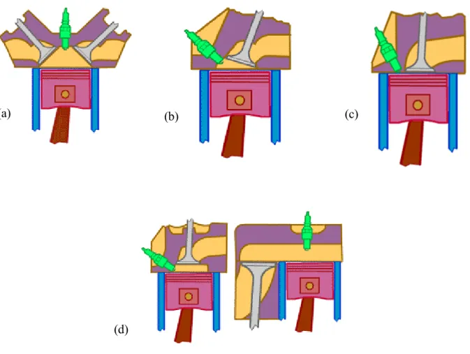
Illustrations of each of the most commons examples ICE chamber shapes which produces a “fast burn” will be given next (Figure 5),
Figure 5 – Example of common internal combustion engine chambers: (a) hemispherical chamber; (b) wedge shaped chamber; (c) bathtub chamber; (d) bowl & piston with flathead on the right. [6]
(a)
(b)
(c)
In the scilab's program it was assumed that the combustion chamber was the simplest possible, so the piston is flat on top, the location of the spark plug is in the middle of the cylinder between the valves and the combustion chamber has a cylindrical geometry. Using this shape and knowing that the combustion reaction is so quick, it is possible to assume that the mean burned gas front can also be approximated by a cylinder instead by a sphere without committing significant errors as regards overall performance
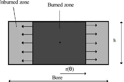
b) Combustion chamber considerations
Assuming that the burned zone is a cylinder of height,
h
and radius,r
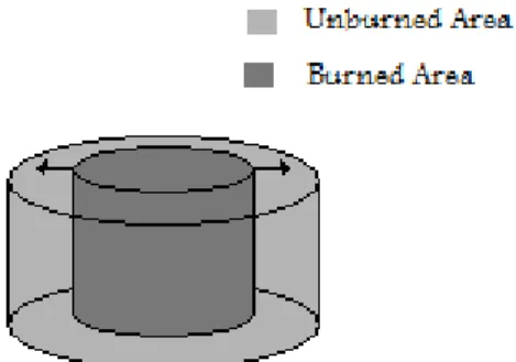
at any instant of θ and using the model which consists in a two zone analysis of the combustion chamber which contains an unburned and burned gas region separated by a turbulent flame front (Figure 6),Figure 6 – Sketch of the front shape of the combustion chamber
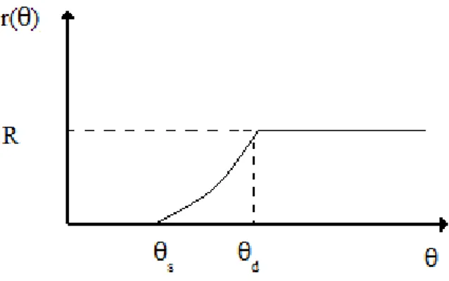
It is possible to predict how the radius, r is going to change during the flame travel, assuming a linear distribution as it will be explained next.
The variation of the burned radius due to the change of the crank angle can be expressed by the approximation (Figure 7),
Bore
Unburned zone
Burned zone
Figure 7 - Schematic of burned radius as a function of the crank angle
where
R=
bo
2
, and
d is the angle
at which the burned gas cylinder reaches the enginecylinder wall.
d is determined by the flame speedV
f (in terms of angular rates), Then,r =
dr
d
=0
for
sr =
V
f−
s
anddr
d
=
V
f for
s
dr=R
anddr
d
=0
for
dThe flame speed
V
f is given by the turbulence model. See “Appendix A.4” forr
mathematicaldevelopment.
Being
h=h
the height from piston, at any instant of θ, to the top of the cylinder, comesh=
v
∗
R
2
(2.14)where
v
is the total volume of the cylinder.The burned and unburned volume and mass are easy to predict, now that
r
andh
areknown.
The burned volume is,
V
b=∗
h∗r
2 (2.15)so
V
b=
1
R
2v∗r
2
(2.16) and its derivative
dV
bd
=
1
R
2r
2dv
d
2∗v∗r
R
2dv
d
(2.17)the unburned volume comes,
V
u=
v−V
b (2.18)Finally, assuming that
m
b is proportional toV
b , it is possible to say,m
bm
=
V
bv
(2.19)then, the burned mass is
mb=m v Vb (2.20) its derivative
dm
bd
=
m∗
1
v
dV
bd
−
V
bv
2dv
d
(2.21)and the unburned mass is
m
u=
m−m
b (2.22) and its derivativedm
ud
=
−
dm
bd
(2.23)c) Thermodynamic model
The energy balance on the unburned zone is
dU
udt
= ˙
Q
u−
P.
dV
uwhere
dm
udt
= ˙
M
u=− ˙
M
b ,M
˙
u is the mass transfer rate to the unburned zone andM
˙
b is themass transfer rate to the burned zone;
Q
˙
u is the heat transfer rate from the unburned zone to the walls; P is the pressure in the cylinder; Vu the unburned volume; and Uu is the total internalenergy in the unburned zone.
After the algebraic manipulation explained in “Appendix A.5” this equation becomes,
M
u∗
Cv
udT
udt
= ˙
Q
u−
P
dV
udt
˙
M
b∗
Cv
u−
Cp
u∗
T
u(2.25)
The energy balance for the burned zone is
dU
bdt
= ˙
Q
b−
P.
dV
bdt
˙
M
b∗
h
u (2.26)where
dm
bdt
= ˙
M
b ; whereQ
˙
b is the heat transfer rate from the burned zone to the walls; Vband
U
b are the volume and internal energy of the burned zone. The mass balances are˙
M
b=
dM
bdt
(2.27) and˙
M
u=
−
dM
bdt
(2.28)where
M
b andM
u are the zone masses.After the algebraic manipulation explained in “Appendix A.6” equation (2.26) becomes,,
M
b∗
Cv
bdT
bdt
= ˙
Q
b−
P
dV
bdt
˙
M
b∗
Cp
u∗
T
u−
Cv
b∗
T
b
hf
u−
hf
b
(2.29)(3) Combustion termination
r =R
If the end of the combustion process is progressively delayed by retarding the spark timing, or decreasing the flame speed by decreasing the piston speed, the peak cylinder pressure occurs later in the expansion stroke and is reduced in magnitude. These change reduce the expansion stroke work transfer from the cylinder gases to the piston.
2.3.2 Turbulence characteristics
The flow processes in the engine cylinder are turbulent. In turbulent flows, the rates of transfer and mixing are several times greater than the rates due to molecular diffusion. This turbulent flow is produced by the high shear flow set up during the intake process and modified during compression. It leads to increased rates of heat, mass transfer and flame propagation, so, is essential to the satisfactory operation of the ICE.
This section explains the structure of the turbulent engine flame in the combustion process, as it develops from the spark discharge and the speed at which it propagates across the combustion chamber.
The turbulence model is based on equations that describe the evolution of turbulence in a fluid where the density is a function only of time. For details see [2].
The turbulence kinetic energy per unit mass,
k
is described by,dk
dt
=
P−D
1
M
c
I−E −k
dM
cdt
(2.30)During the burn stage the turbulence energies of the burned and unburned gases are tracked together using the above equation with just the P and D terms,
dk
dt
=
P−D
(2.31)because during the combustion there is no mass transfer, so
dM
cfunctions of
dM
cdt
.The term P is the turbulence energy production rate per unit mass and is modeled by,
P=F
pA
wv
∣
U
3∣
−
2
3
k
1
v
dv
dt
(2.32)where the first term accounts for turbulence production due to the strain in the shear flow on the walls and the second the effects of compression.
D is the turbulence energy dissipation rate per unit mass and is modeled by,
D=F
dkV
tv
1 /3 (2.33)The coefficients
F
p and Fd are parameters that can be set by reference to experiments. Toget the respective values for each term, the Engine Simulation Program (ESP) which is available in the Internet at the site “http://esp.stanford.edu/” was referenced.
Using the turbulence equation and the next two equations, it is possible to estimate
V
f which is the velocity of the flame front relative to the unburned gases,k =
V
t2
2
(2.34)and
V
f=
V
L
C
f∗
V
t (2.35)where
V
t is the turbulence velocity in the unburned zone,V
L is the specified laminar flame speedand
C
f is a specified coefficient, approximately unity. The value forV
L was obtained from theESP.
After having the
V
f estimated, it is possible to make a realistic approximation to the real variation of the burned radius. Knowing that,dr
and
dt=
1
w
d
comes,dr
d
=
V
fw
(2.37)Finally, the real variation of the burned radius due to the change of the crank angle when
s
d can be expressed by the next equation,r =
V
fw
−
s
(2.38) anddr
d
=
V
fw
for
s
d (2.39)2.3.3 Heat Transfer
The heat transfer model used in this report is the same as before.
However, since we are using the two zone combustion model, during the development of the combustion, different quantities of heat are released from the burned and unburned zone.
Applying the Newtonian convection equation,
Q=h
g
A
w
T −T
w/
N
(2.40)The only thing that will change in this two zone combustion model are the exposed burned and unburned areas as shown in figure 8.
The exposed burned area varies in function of the burned radius,
Awb=∗r2 (2.41) the exposed unburned area comes,
Awu=Aw−Awb (2.42) Finally, the heat transfer equation for the the burned zone is,
Q
wb=−
hg∗A
wb∗
T
b−
T
w/
N
(2.43) where,hg=300∗P0.75∗U0.75∗bo−0.25∗Tb−0.465/1000 (2.44)
and the heat transfer equation for the unburned zone is,
Q
wu=−
hg∗A
wu∗
T
u−
T
w/
N
(2.45) where,h
g=300∗P
0.75∗
U
0.75∗
bo
−0.25∗
T
u −0.465/
1000
(2.46)where the units of hg, P, U, b and T are kW/m2K, kPa, m/s, m and K, respectively. The piston speed, U
is given by equations (2.9) and (2.10).
2.4. Completely burned gas expansion
The burning stage lasts until the piston has progressed beyond TC, but ends before the piston has
descended to the point of
=
evo near BC. The expansion from the end of combustion to
evo2.4.1 Thermodynamic equation of burned gas expansion
During this stage, the energy balance on the in-cylinder gas is,
dU
d
=
Q−
W
(2.47)As both valves are closed there is no mass exchange so
dm
d
=
m
i=
m
e=0
(2.48)After the algebraic manipulation shown in “Appendix A.7” comes,
dT
d
=
Q
m∗Cv
−
R
bT
CvV
dV
d
(2.49)2.4.2 Heat Transfer
At this stage, the heat release rate at any crank angle θ to the exposed cylinder wall at an engine speed N is determined with a Newtonian convection equation,
Q=h
g
A
w
T −T
w/
N
(2.50)The heat transfer coefficient hg(θ) is the instantaneous averaged heat transfer coefficient and
A
w is the exposed cylinder area.The instantaneous heat transfer coefficient during the expansion stage is estimated in the same way as the heat transfer coefficient in the compression stage.
where the units of hg, P, U, b and T are kW/m2K, kPa, m/s, m and K, respectively. The piston speed, U
Chapter 3 – Gas exchange cycle
This cycle deals with the fundamentals of the gas exchange process, intake and exhaust and the valves mechanism in a four stroke internal combustion engine, called the gas exchange cycle . Only a brief explanation about the thermodynamics state and gas flow rate will be given.
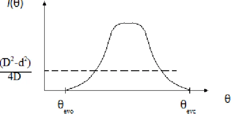
This cycle is called the gas exchange cycle because it is where the burned gases from the expansion stroke are expelled (exhaust stroke, =evo≈2 to θ=3π) and fresh fuel-air is ingested (ingested stroke, ivo to =4 ).
This cycle is also described by the main two laws of thermodynamics governing the unburned and burned fuel-air mixture in the cylinder.
The gas exchange process is based on a “perfect valve timing”. In perfect valve timing the exhaust valve closes exactly when the cylinder pressure drops below exhaust system pressure, but after TC at
=3 . Then both valves remain closed while the piston descends (expanding the cylinder volume) until the cylinder pressure reaches the intake system pressure, which is less than the exhaust pressure for unsupercharged engines.
3.1.Valve action
Valves allow the gas exchange to occur. Valve opening and closing control is called valve timing. The valves action occurs for the following values of θ,
● exhaust valve opens (evo) at =evo=2 −/9 ;
● exhaust valve closes (evc) at =evc=3 ;
● intake valve opens (ivo) at
=
ivo determined by intake pressure; ● intake valve closes (ivc) at =evo=4 .3.1.1 Geometry
The valves are driven by a cam that rotates at half the speed of the crankshaft.
The valve flow area depends on valve lift and the geometric details of the valve head, seat and stem.
Curtain area=∗D∗l
(3.1) andPort area=
1
4
D
2−
d
2
(3.2)where
l=l
is the valve lift, D the port diameter and d the stem diameter. It can be written mathematically as,A
v=
min D l ,
1
4
D
2
−
d
2
(3.3)The valve lift,
l
is usually a curve that looks like figure 9,Figure 9 - Typical exhaust valve timing diagram Approximating this curve by the formula,
l =
l
m2
1−cos
(3.4)where
l
m is the maximum valve lift and usuallyl
m
D
2
−
d
2
3.1.2 Isentropic flow thought an orifice
From the gas dynamics, the isentropic flow through an orifice is given by,
m=
o∗
C
f∗
A
v∗
c
o∗
2
k −1
P
vP
o
2k−
P
vP
o
k1k
12 (3.6) as long as,P
oP
v
P
oP
v
cr=
k1
2
k k1 (3.7) ifP
oP
v≥
P
oP
v
cr (3.8) then
m=
m
cr=
o∗
C
f∗
A
v∗
c
o∗
k 1
2
k2 k11 (3.9) WhenP
oP
v≤
P
oP
v
crthe flow is “choked”. This means that the flow right at the orifice (the valve passage) is “sonic”. At this
condition only mcr (=constant) can pass through the valve passage regardless of how small we
make
P
vP
o(see figure 10). Note that
P
o is the upstream pressure (stagnation pressure) andFigure 10 – Isentropic flow through an orifice
For an ideal gas,
o=
P
oR∗T
o(3.10) and
c
o is the speed of sound,co=
kRTo (3.11)Note that the speed of sound goes up with the upstream temperature. And note that the upstream for exhaust is the cylinder temperature and the upstream for intake is the manifold temperature which is much less than cylinder temperature. That is why exhaust valve is smaller than intake valve.
The non-ideal effects are accounted by introducing a flow coefficient Cf, which is here assumed to
be Cf≈0.40 .
3.2. Exhaust stage
The configuration of the exhaust system plays an important role for a good engine performance. The exhaust system typically consists of an exhaust manifold, exhaust pipe, often a catalytic converter for emission control, and a muffler or silencer. My study concerns only with the exhaust stroke which proceeds the power stroke cycle.
At the end of the power stroke, the piston is located at the bottom center, θ=2π . Heat that is left over from the power stroke is now transfered to the water in the water jacket until the pressure approaches atmospheric pressure. The exhaust valve is then opened by the cam on the rocker arm to begin the exhaust stroke.
another ignition cycle. As the exhaust stroke begins, the cylinder and combustion chamber are full of exhaust products at low pressure. Because the exhaust valve is open, the exhaust gas is pushed past the valve and exits the engine.
3.2.1 Thermodynamics Model of the Exhaust stage
As it was said, this stroke is also described by the main two laws of thermodynamics. The energy balance for the exhaust stroke is,
dU
d
=
Q−
W −
H
e (3.12)As the intake valve is closed there is no mass exchange trough it so
m
i=
H
i=0
and as theexhaust valve is opened comes
dm
d
=−
m
e .After the algebraic manipulation shown in “Appendix A.8” comes,
dT
d
=
Q
m∗C
vb
−
R
b∗
T
V ∗C
vb
dV
d
−
m
bm
R
b∗
T
C
vb (3.13)3.2.2 Heat transfer
At this stage, the heat release rate at any crank angle θ to the exposed cylinder wall at an engine speed N is determined with a Newtonian convection equation,
Q=h
g
A
w
T −T
w/
N
(3.14)The heat transfer coefficient hg(θ) is the instantaneous averaged heat transfer coefficient and is the
exposed cylinder area.
The instantaneous heat transfer coefficient during the expansion stage is estimated in the same way as the heat transfer coefficient in the compression stage.
h
g=300∗P
0.75
∗
U
0.75∗
bo
−0.25∗
T
b−0.465
/
1000
(3.15)where the units of hg, P, U, b and T are kW/m2K, kPa, m/s, m and K, respectively. The piston
speed, U is given by equations (2.9) and (2.10).
2.3. Intake stage
The exchange cycle ends with the intake stroke as the piston is pulled towards the crankshaft (to the bottom center position, BC) as the intake valves opens and fuel (unburned gas) and air are drawn past it and into the combustion chamber and cylinder from the intake manifold located on top of the combustion chamber. The exhaust valve is closed and the electrical contact switch is open. The fuel/air mixture is at a relatively low pressure (near atmospheric). At the end of the intake stroke, the piston is located at the bottom center position, ready to begin the power cycle.
Intake manifolds consisting of plenums (separated spaces containing air at a pressure greater than atmospheric pressure) and pipes are usually required to deliver the inlet air charge from some preparation device such as an air cleaner or compressor.
3.3.1 Thermodynamics Model of the Intake stage
Using the main two laws of thermodynamics, the energy balance for the intake stroke is,
dU
d
=
Q−
W
H
i (3.18)As the exhaust valve is closed there is no mass exchange trough it so
m
e=
H
e=0
and as theintake valve is opened comes
dm
d
=
m
i .After the algebraic manipulation shown in “Appendix A.9” comes,
dT
d
=
Q
m∗C
vu−
R
u∗
T
V ∗C
vudV
d
m
u
m∗C
vu
C
pu∗
T
u−
C
vu∗
T
(3.19)3.3.2 Heat transfer
The heat transfer model for the intake is the same as it was explained for the exhaust process. Note that in the intake process the heat transfer can be neglected, when comparing it to the heat released in the exhaust and combustion stages.
As it was said, the computer simulation was implemented by way of “Scilab” computer program. “Scilab” is a scientific software for numerical computations, and it is currently used in educational and industrial environments around the world. This program can be found freely in the following website: http://www.scilab.org/
The ICE computer simulation developed is called CycleComQC (see appendix C.1) and the original one developed by CVK is called CycleCom (see appendix C.2).
CycleComQC Inputs
The values of the input parameters used in this simulation can be found in the tables below. Engine data:
Exhaust valve data:
Connecting rod/stroke length ratio 2 /
Compression ratio 11 /
Maximum cylinder volume 0.00055
Ignition onset rad
Burn duration rad
Burning end rad
Engine rpm rpm 6000 rpm
Cylinder wall temperature 400 K
Rc rc Vm m3 ths 0.88π thb 0.33π thd 1.21π Tw
Exhaust valve opens thevo rad
Exhaust valve closes thevc rad
Exhaust port diameter eportd 0.040 m
Exhaust valve stem diameter estem 0.015 m
Exhaust valve max lift elm 0.035 m
2π-π/9 3π
Intake valve data:
Intake-exhaust state
Unburned fuel-air equation of state, CH4:
Burned fuel-air equation of state, CH4:
Intake valve opens 3π rad
Intake valve closes 4π rad
Intake port diameter 0.040 m
Intake valve stem diameter 0.015 m
Intake valve max lift 0.035 m
thivo thivc iportd istem ilm Intake pressure Pi 100 K Exhaust pressure Pe 150 K Intake temperature Ti 320 K
Uf-air gas constant Ru 0.2968 kJ/kgK
Cp for uf-air Cpu 1.022 kJ/kgK
Specific heat ration for uf-air ku 1.409 /
Zero degree enthalpy of uf-air hfu -692.0 kJ/kg
Cv for uf-air Cvu 0.725 kJ/kgK
Bf-air gas constant Rb 0.2959 kJ/kgK
Cp for bf-air Cpb 1.096 kJ/kgK
Specific heat ration for bf-air kb 1.370 /
Zero degree enthalpy of bf-air hfb -3471.0 kJ/kg
Turbulence coefficients:
Parameters set by reference to experiments 0.03 /
Parameters set by reference to experiments 0.05 /
Coefficient set by reference to experiments 0.4 /
Laminar flame speed 0.04 m/s
Fd F
p
Cf VL
Results/Discussion
The single zone with homogeneously mixed burned and unburned gases developed by CVK is called the single zone adiabatic model. I have added heat transfer to this model and it will be called the single zone heat transfer model so first the results obtained from the single zone heat transfer model simulation program (see appendix C.3.) are discussed. After that, it is discussed the main simulation program and how the power, efficiency and heat transfer vary with the engine speed and how this have influence on the engine performance. Another point explained is the turbulence model and how it affects the combustion stage.
As illustration an engine with a compression ratio of 11, total volume of 55 cm3, using methane
(CH4) which properties are very similar to gasoline and setting the engine to run at 6000rpm was
obtained the following results for the heat transfer model,
Figure 12 - P-V diagram for a four stroke engine running at 6000rpm
In order to compare the performance of an adiabatic engine with a non-adiabatic engine, the following results were obtained,
Figure 14 – Variation of the power, efficiency and work with the engine speed (rpm) for an adiabatic engine
Figure 15 – Variation of the power, efficiency and work with the engine speed (rpm) for a non-adiabatic engine
As we can see, the heat loss affects the engine performance. As we were expecting, the power, efficiency and the work drops when we have a non-adiabatic engine. In a non-adiabatic engine the temperature and pressure is smaller than in an adiabatic engine due to the greater heat losses which represents work that cannot be done.
Note that as the engine speed increases, the work drops off because the amount of gas burned goes down. At high engine speed the burn gas exchange is restricted by the flow through the valves. In particular the exhaust gases can not be completely expelled. Hence the amount of intake gases is reduced. Also the work required for pumping of the intake and exhaust, especially exhaust is greatly increased.
For a non-adiabatic engine
RPM
Power (kW)
Efficiency (%)
Work (kJ)
3000 12.40 0.40 0.50 4000 13.79 0.38 0.41 5000 14.05 0.37 0.34 6000 13.66 0.35 0.27 7000 13.00 0.32 0.22 8000 13.58 0.34 0.20
For an adiabatic engine
RPM
Power (kW)
Efficiency (%)
Work (kJ)
3000 14.81 0.49 0.59 4000 16.32 0.47 0.49 5000 16.60 0.46 0.40 6000 16.22 0.43 0.32 7000 15.57 0.41 0.27 8000 14.84 0.39 0.22
The results from the last version of the CycleComQC are the followings,
Figure 16 – Variation of the power, efficiency,work and heat loss with the engine speed (rpm) for a non-adiabatic engine Comparing this values for the final program with the ones obtained in heat transfer model, we conclude that the values for the efficiency are to high. For 6000rpm, the efficiency result obtained for this final simulation doing Q=0 is 77%. This cannot be correct because it exceeds Carnot efficiency which is only approximately 60%. This confirms that something is wrong with the basic two zone model we have developed. However, we will show the results obtained by this model.
RPM
Power (kW)
Efficiency (%)
Qt (kW)
Work (kJ)
Qw (kW/rad)
2000 8.90 40.0% -10.60 0.534 -0.636 3000 13.52 43.1% -14.98 0.541 -0.599 4000 17.89 47.2% -19.03 0.537 -0.571 5000 21.85 52.1% -22.79 0.524 -0.547 6000 25.24 57.4% -26.21 0.505 -0.524 7000 27.55 62.8% -28.91 0.472 -0.496 8000 27.93 67.5% -30.05 0.419 -0.451 9000 26.71 69.7% -29.75 0.356 -0.397 10000 24.38 68.8% -28.43 0.293 -0.341 11000 21.38 65.1% -26.52 0.233 -0.289 12000 18.04 59.1% -24.29 0.180 -0.243
Figure 17 – Power as a function of engine speed (rpm)
As expected, the power rises and falls with rpm, but the peak occurs for 8500rpm which is much too high. Also the peak power is much too large.
When we have heat loss in an engine, occurs a reduction in its temperature and pressure which represents work that cannot be done leading to lower values of power.
Figure 18 – Efficiency as a function of engine speed (rpm)
3000 4000 5000 6000 7000 8000 9000 10000 11000 12000 0.00 5.00 10.00 15.00 20.00 25.00 30.00
![Figure 1 – Four stroke internal combustion engine. [5]](https://thumb-eu.123doks.com/thumbv2/123dok_br/15242880.1023208/11.918.275.657.96.526/figure-stroke-internal-combustion-engine.webp)
![Figure 2 - A four-stroke spark ignition cycle. [5]](https://thumb-eu.123doks.com/thumbv2/123dok_br/15242880.1023208/12.918.187.716.395.691/figure-four-stroke-spark-ignition-cycle.webp)