Sovereign debt effects and composition : evidence from time-varying estimates

António Afonso,

João Tovar Jalles

Sovereign Debt Effects and Composition:

Evidence from Time-Varying Estimates

WP03/2017/DE/UECE _________________________________________________________

W

P

S

OVEREIGN

D

EBT

E

FFECTS

A

ND

C

OMPOSITION

:

E

VIDENCE

F

ROM

T

IME

-V

ARYING

E

STIMATES

António Afonso

_{João Tovar Jalles}

Abstract

We compute time-varying responses of the sovereign debt ratio to primary budget balances for 13 advanced economies between 1980 and 2012, and assess how fiscal sustainability reacts to different characteristics of government debt. We find that the fiscal sustainability time-varying coefficient increases the higher the share of public debt denominated in foreign currency. Moreover, the countries become more sustainable if they contract a higher share of long-term public debt, if it is held by the central bank or if it is easily marketable.

JEL: C23, E62, F34, H63

Keywords: sovereign debt, fiscal sustainability, time-varying coefficients, debt composition

* _{The opinions expressed herein are those of the authors and do not reflect those of their employers.}

$ _{ISEG/UT - University of Lisbon, Department of Economics; UECE – Research Unit on Complexity and} Economics. R. Miguel Lupi 20, 1249-078 Lisbon, Portugal. UECE is supported by FCT (Fundação para a Ciência e a Tecnologia, Portugal), email: aafonso@iseg.utl.pt.

# _{Centre for Globalization and Governance, Nova School of Business and Economics, Campus Campolide,} Lisbon, 1099-032 Portugal. email: joaojalles@gmail.com. UECE – Research Unit on Complexity and Economics. R. Miguel Lupi 20, 1249-078 Lisbon, Portugal.

2

“In countries with fiscal space, the budget could also do more to support aggregate demand. Many countries lack this fiscal space and, of course, how much countries can do to support demand will depend on individual country circumstances.” In Act Now, Act Together, IMF 20161

1. Introduction

When assessing fiscal sustainability, studies traditionally use overall government debt without considering its composition or set of possible characteristics. In fact, several features of sovereign debt can provide relevant information to capital markets when pricing both new issuances and secondary market transactions. Moreover, the possibility that fiscal sustainability is also a time-varying reality is important and a scarcely an issue addressed in the related literature.

Several papers have used a so-called fiscal reaction function to assess, in a forward-looking way, if larger primary surplus today lead to a reduction in the future level of debt (see notably Bohn, 1998, Canzoneri, Cumby and Diba, 2001, Afonso, 2008, Weichenrieder and Zimmer, 2014, whose evidence points to the lack of adherence to the idea that price level may be determined via the intertemporal government budget constraint, given that governments are in fact quite Ricardian). In another strand, for instance, Dell’Erba, Hausmann and Panizza (2013) report that debt composition matters for sovereign bond yield spreads, while Kim (2015) shows that long-term government debt ends up being less expensive than short-term debt, and it implies a higher limit for debt issuance without default.

3

As Ostry el al. (2010) put it, what constitutes a safe level of sovereign debt or ample fiscal space is very difficult to pin down precisely in practice, and can never be established through some mechanical rule or thresholds. We add two contributions to the literature: first, we compute a set of time-varying fiscal responses of the debt-to-GDP ratio to primary budget balances for a sample of 13 advanced countries, which we take as a measure of fiscal space; second, we assess how these time-varying so-called sustainability coefficients react to several composition features and characteristics of government debt, notably in terms of currency denomination, maturity, and the holders of the sovereign debt (type of lender). This is important since there is a strict relationship between the notion of fiscal space and government bond yields (spreads) which are directly linked to risk perception and features of financial volatility dynamics (Ribeiro et al., 2016).

The remainder of the paper is organized as follows. Section 2 describes the underlying data and empirical methodology to be used. Section 3 presents and discusses our main results. The last section concludes.

2. Methodology and Data

Our sample covers 13 Advanced Economies with annual data between 1980 and 2012. The country set is: Australia, Spain, Ireland, Japan, Canada, Sweden, Netherlands, Italy, Germany, France, Belgium, UK and USA. We begin by estimating what we call a country-specific time-varying fiscal sustainability coefficient ( ). Therefore, we start with the following fiscal reaction function:

i i i i i d pb    (1)

4

where pb is the primary balance-to-GDP ratio and d is the sovereign debt-to-GDP ratio (both variables are retrieved from the IMF’s International Financial Statistics). Note that is our coefficient of interest and it measures the country-specific sensitivity of the primary balance to public debt changes, which may vary over time. The magnitude of  conveys notably a message to investors regarding the likelihood of a certain sovereign issuer being closer of further away to fiscal distress, which then will have to be translated into different yield and CDS spreads. denote country and time effects, respectively. Finally, is an i.i.d. disturbance term satisfying standard assumptions of zero mean and constant variance.

The coefficient in (1) is then assumed to change slowly and unsystematically over time and the expected value of the coefficient at time t is equal to the value of the coefficient in time t-1 (i.e. we assume the coefficient to be a random walk). The change of the coefficient is denoted by , which is assumed to be normally distributed with expectation zero and variance :

. (2)

We estimate (1) and (2) jointly using the Varying-Coefficient model proposed by Schlicht (1985, 1988). In this approach the variances are calculated by a method-of-moments estimator that coincides with the maximum-likelihood estimator for large samples. The model described in (1) and (2) generalizes the classical linear regression model, which is obtained as a special case when the variance of the disturbances in the coefficients approaches to zero. As discussed by Aghion and Marinescu (2008), this method has several

5

advantages compared to other methods to compute time-varying coefficients (TVC) such as rolling windows and Gaussian methods. First, it allows using all observations in the sample to estimate the magnitude of spillover in each year. Second, changes in the size of estimated TVC in a given year come from innovations in the same year, rather than from shocks occurring in neighbouring years.

As a second step, we use the computed time-varying estimates - the fiscal sustainability TVC which one can proxy as a measure of fiscal space - as our dependent variable in a regression using public debt characteristics in the right hand side. Together with a set of controls known to affect fiscal developments (see for instance, Afonso, 2003, and Golinelli and Momigliano, 2008) we look at the positive/negative effects of the several dimensions of government debt on the fiscal sustainability position or our measure of fiscal space. In particular, we estimate:













where is our measure of fiscal space, and an indication of future possible fiscal concern, in country i at time t. represents country fixed effects; denotes time effects. The former captures unobserved heterogeneity across countries and time-unvarying factors such as geographical variables; the latter aims to control for global shocks. X is a vector of control it variables that includes real GDP growth, inflation rate, trade openness (exports plus imports over GDP), the budget balance-to-GDP ratio (all of these retrieved from the IMF’s

6

International Financial Statistics) and an institutional quality proxy(given by the polity2 indicator of the Polity IV project).2 Finally,

it

DC corresponds to a vector containing our set of public debt characteristics (see below). it is an error term disturbance satisfying standard assumptions.

Equation (3) is first estimated by Ordinary Least Squares (OLS). Since the dependent variable in equation (3) is based on estimates, the regression residuals can be thought of as having two components. The first component is sampling error; the second component is the random shock that would have been obtained even if the dependent variable were observed directly as opposed to estimated. This would lead to an increase in the standard deviation of the estimates, lowering the t-statistics. This means that any correction to the presence of this unmeasurable error term will increase the significance of our estimates. To address this, equation (3) is estimated using Weighted Least Squares (WLS). Specifically, the weighted-least-squares estimator assumes that the errors it in equation (3) are distributed as

) / , 0 ( 2 i it N  s

  , where is the estimated standard deviation of the TVC coefficient in country i, and _2 _{is an unknown parameter that is estimated in the second-stage regression.}

The indicators on the composition of sovereign debt are sourced from Abbas et al. (2014) and cover four major dimensions: 1) currency, i.e. the share of debt issued in foreign currency versus local currency; 2) maturity, i.e. the share of short-term debt (with a maturity of less than one year or the shortest maturity of more than one year for which data are available at the date of issuance) versus medium- and long-term debt; 3) holders, i.e. the share of the debt that is held by either the central bank, the domestic commercial banks,

7

residents, or the domestic non-bank sector; and 4) marketability, i.e. the share of the debt that is non-marketable versus marketable. All shares are in percentage of total government debt.

3. Analysis of Empirical Results

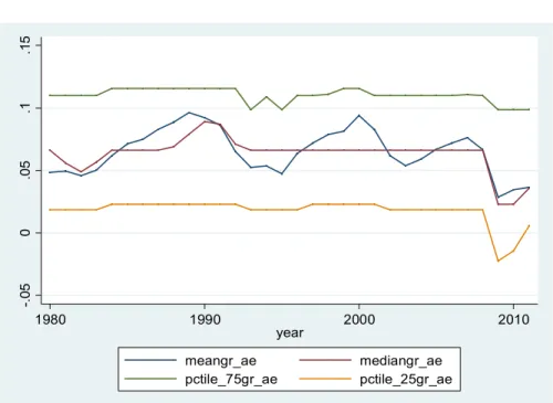
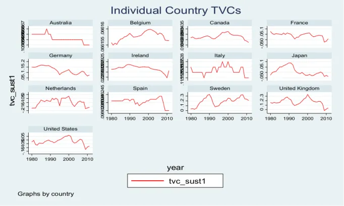
Overall, the results of the first step of our analysis – estimating the country-specific TVCs – show that our coefficient fluctuates around a median of 0.065 (Figure 1). Moreover, the time varying sustainability coefficient fell significantly following the Global Financial Crisis. This is even more evident for the individual country’s TVCs (Figure 2).

Figure 1: Interquartile range of Fiscal Sustainability Time-Varying Coefficient Estimates, Whole Sample (1980-2012)

-.0 5 0 .0 5 .1 .1 5 1980 1990 2000 2010 year meangr_ae mediangr_ae pctile_75gr_ae pctile_25gr_ae

8

Figure 2: Country-by-country time profile of Fiscal Sustainability Time-Varying Coefficient Estimates (1980-2012) .1 09 86 4 .1 09 86 5 .1 09 86 6 .1 09 86 7 .0 66 15 5 .0 66 16 .0 18 42 .0 18 42 5 .0 18 43 .0 18 43 5 -.0 50 .0 5. 1 .0 5. 1. 15 .2 .0 22 91 .0 22 91 5 .0 22 92 .0 22 92 5 .1 15 52 5 .1 15 52 6 .1 15 52 7 .1 15 52 8 -.0 50 .0 5. 1 -.2-.1 5-.1-.0 50 .0 98 62 35 .0 98 62 4 .0 98 62 45 0 .1 .2 .3 0 .1 .2 .3 -.1 5-.1-.0 50. 05 1980 1990 2000 2010 1980 1990 2000 2010 1980 1990 2000 2010 1980 1990 2000 2010

Australia Belgium Canada France

Germany Ireland Italy Japan

Netherlands Spain Sweden United Kingdom

United States tvc_sust1 tv c_ su st 1 year Graphs by country

Individual Country TVCs

Source: author’s computations.

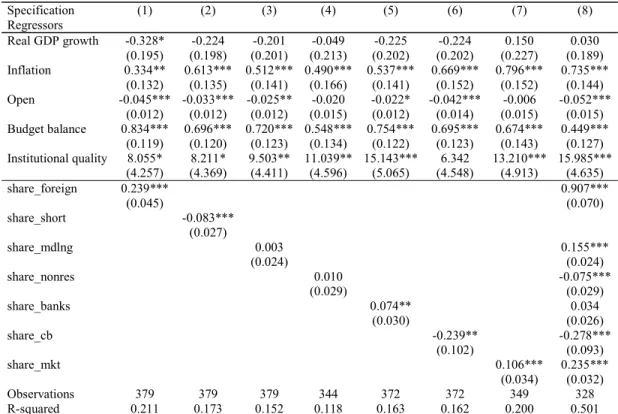
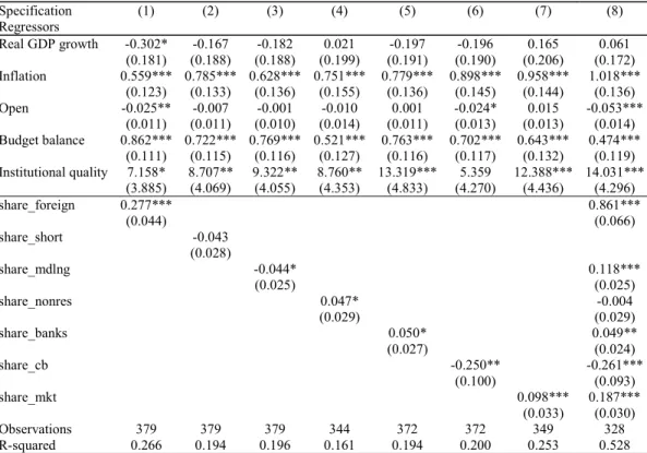
We then move on to estimate our equation (3) and assess the relevance of several public debt characteristics in affecting our measure of fiscal space. The estimations via OLS and WLS are reported in Table 1 and in Table 2, respectively.

Our set of results merit several comments. The larger the share of sovereign debt issued in foreign currency the higher the fiscal sustainability time-varying coefficient (and naturally the further away form a situation of distress that sovereign would be). The larger (smaller) the share of short-term debt (medium/long-term) the smaller (higher) the fiscal sustainability TVC.

9

Table 1. Ordinary Least Squares

Specification (1) (2) (3) (4) (5) (6) (7) (8) Regressors Real GDP growth -0.328* -0.224 -0.201 -0.049 -0.225 -0.224 0.150 0.030 (0.195) (0.198) (0.201) (0.213) (0.202) (0.202) (0.227) (0.189) Inflation 0.334** 0.613*** 0.512*** 0.490*** 0.537*** 0.669*** 0.796*** 0.735*** (0.132) (0.135) (0.141) (0.166) (0.141) (0.152) (0.152) (0.144) Open -0.045*** -0.033*** -0.025** -0.020 -0.022* -0.042*** -0.006 -0.052*** (0.012) (0.012) (0.012) (0.015) (0.012) (0.014) (0.015) (0.015) Budget balance 0.834*** 0.696*** 0.720*** 0.548*** 0.754*** 0.695*** 0.674*** 0.449*** (0.119) (0.120) (0.123) (0.134) (0.122) (0.123) (0.143) (0.127) Institutional quality 8.055* 8.211* 9.503** 11.039** 15.143*** 6.342 13.210*** 15.985*** (4.257) (4.369) (4.411) (4.596) (5.065) (4.548) (4.913) (4.635) share_foreign 0.239*** 0.907*** (0.045) (0.070) share_short -0.083*** (0.027) share_mdlng 0.003 0.155*** (0.024) (0.024) share_nonres 0.010 -0.075*** (0.029) (0.029) share_banks 0.074** 0.034 (0.030) (0.026) share_cb -0.239** -0.278*** (0.102) (0.093) share_mkt 0.106*** 0.235*** (0.034) (0.032) Observations 379 379 379 344 372 372 349 328 R-squared 0.211 0.173 0.152 0.118 0.163 0.162 0.200 0.501

Note: Dependent variable is the TVC estimate. OLS estimation. Robust clustered standard errors in parenthesis. Constant term estimated but omitted for reasons of parsimony. *, **, *** denote statistical significance at the 10, 5 and 1 percent levels, respectively.

Moreover, we also find that the larger (smaller) the share of debt held by the central bank (commercial banks) the smaller (higher) the fiscal sustainability TVC. In this context, we can bear in mind that several countries in our sample have benefited from the Quantitative Easing measures of the respective central banks, which allowed both additional demand in capital markets for those sovereign bonds, together with lower spreads. For instance, in the third quarter of 2012 the European Central Bank announced that it could conduct Outright Monetary Transactions in secondary sovereign bond markets, and other similar Quantitative Easing procedures were also implemented earlier on by other central

10

banks.3 _{Hence, a higher share of central bank holdings of sovereign debt might be perceived}

by investors with mixed feelings, regarding countries’ ability to fund themselves in the market. Finally, the larger the share of marketable debt the higher the fiscal sustainability TVC, which also would link to the fact that such sovereign debt can have a higher degree of liquidity in the markets.

Table 2. Weighted Least Squares

Specification (1) (2) (3) (4) (5) (6) (7) (8) Regressors Real GDP growth -0.302* -0.167 -0.182 0.021 -0.197 -0.196 0.165 0.061 (0.181) (0.188) (0.188) (0.199) (0.191) (0.190) (0.206) (0.172) Inflation 0.559*** 0.785*** 0.628*** 0.751*** 0.779*** 0.898*** 0.958*** 1.018*** (0.123) (0.133) (0.136) (0.155) (0.136) (0.145) (0.144) (0.136) Open -0.025** -0.007 -0.001 -0.010 0.001 -0.024* 0.015 -0.053*** (0.011) (0.011) (0.010) (0.014) (0.011) (0.013) (0.013) (0.014) Budget balance 0.862*** 0.722*** 0.769*** 0.521*** 0.763*** 0.702*** 0.643*** 0.474*** (0.111) (0.115) (0.116) (0.127) (0.116) (0.117) (0.132) (0.119) Institutional quality 7.158* 8.707** 9.322** 8.760** 13.319*** 5.359 12.388*** 14.031*** (3.885) (4.069) (4.055) (4.353) (4.833) (4.270) (4.436) (4.296) share_foreign 0.277*** 0.861*** (0.044) (0.066) share_short -0.043 (0.028) share_mdlng -0.044* 0.118*** (0.025) (0.025) share_nonres 0.047* -0.004 (0.029) (0.029) share_banks 0.050* 0.049** (0.027) (0.024) share_cb -0.250** -0.261*** (0.100) (0.093) share_mkt 0.098*** 0.187*** (0.033) (0.030) Observations 379 379 379 344 372 372 349 328 R-squared 0.266 0.194 0.196 0.161 0.194 0.200 0.253 0.528

Note: Dependent variable is the TVC estimate. WLS estimation with weights given by the inverse of the standard errors of the estimated TVCs. Robust clustered standard errors in parenthesis. Constant term estimated but omitted for reasons of parsimony. *, **, *** denote statistical significance at the 10, 5 and 1 percent levels, respectively.

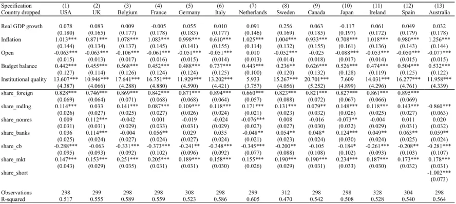
As a robustness exercise, we re-run specification 8 of Table 2, excluding one country at the time from our main sample. The results (in the Appendix), confirm the overall findings

3 _{According to ECB (2015), the announcements of the Outright Monetary Transactions “led to sizeable changes} in the yield curves of some euro area countries”, notably the fall of bond yields in several euro area economies.

11

that we have already reported, notably, and in addition to the main economic drivers, the relevance of the several sovereign debt features (foreign currency debt, shares of longer-term debt, of debt held by the central bank, and of marketable debt).

4. Conclusion

In this paper we have computed time-varying fiscal responses of the debt ratio to primary budget balances for 13 advanced economies and we assessed how countries’ fiscal space reacted to several characteristics of government debt. We found that the fiscal sustainability time-varying coefficient increases with the share of foreign currency debt, the share of longer-term debt, the share of debt held by the central bank, and the share of marketable debt.

From a policy perspective it is quite relevant that fiscal sustainability would diminish with the increase of the share of short-term debt, a situation that tends to arise in distressed economies with long-term debt issuance difficulties in crisis periods, and with some sort of shutdown from capital markets regarding those bonds. In addition, sovereign debt held by the central bank seems to reduce the risks of fiscal concerns, which naturally can also be relevant for the monetary authorities’ policy making, who care notably also about the magnitude of their interventions in the sovereign bond market.

References

Abbas, S., Blattner, L., De Broeck, M., El-Ganainy, A., Hu, M. (2014). “Sovereign Debt Composition in Advanced Economies: A Historical Perspective”, IMF WP/14/162. Aghion, P., I. Marinescu (2008), “Cyclical Budgetary Policy and Economic Growth: What

12

Afonso, A. (2008). “Ricardian Fiscal Regimes in the European Union”, Empirica, 35 (3), 313–334.

Bohn, H. (1998). “The behavior of U.S. public debt and deficits”, Quarterly Journal of Economics 113, 949–963.

Canzoneri, M., Cumby, R., Diba, B. (2001). “Is the Price Level Determined by the Needs of Fiscal Solvency?” American Economic Review, 91(5), 1221-1238.

Dell’Erba, S., Hausmann, R., Panizza, U. (2013). “Debt Levels, Debt Composition, and Sovereign Spreads in Emerging and Advanced Economies”, HKS Faculty Research Working Paper 13-028.

ECB (2015). Research Bulletin 22, Summer 2015.

Golinelli, R., Momigliano, S. (2008). “The cyclical response of fiscal policies in the euro area. Why do results of empirical research differ so strongly?” Banca d’Italia, WP nº 652.

Kim, J. (2015). “Debt Maturity: Does It Matter for Fiscal Space?” IMF WP/15/527.

Ostry, J., Ghosh, A., Kim, J., Qureshi, M. (2010). “Fiscal Space.” IMF Staff Position Note 10/11, IMF, Washington.

Ribeiro, P., Cermeno, R., Curto, J. (2016). “Sovereign bond markets and financial volatility dynamics: Panel GARCH evidence for six-euro area countries”, Finance Research Letters, article in press.

Schlicht, E. (1985). “Isolation and Aggregation in Economics”, Berlin-Heidelberg-New York-Tokyo: Springer-Verlag.

Schlicht, E. (1988). “Variance Estimation in a Random Coefficients Model,” paper presented at the Econometric Society European Meeting Munich 1989.

Appendix

Table A1. Robustness: Weighted Least Squares – dropping one country at the time

Specification (1) (2) (3) (4) (5) (6) (7) (8) (9) (10) (11) (12) (13) Country dropped USA UK Belgium France Germany Italy Netherlands Sweden Canada Japan Ireland Spain Australia Real GDP growth 0.078 0.083 0.009 -0.005 0.055 0.010 0.091 0.256 0.063 -0.117 0.061 0.049 0.032 (0.180) (0.165) (0.177) (0.178) (0.183) (0.177) (0.146) (0.169) (0.185) (0.197) (0.172) (0.179) (0.178) Inflation 1.013*** 0.871*** 1.078*** 1.083*** 0.998*** 0.610*** 1.025*** 1.004*** 0.933*** 0.708*** 1.018*** 0.980*** 1.256*** (0.144) (0.134) (0.137) (0.145) (0.141) (0.155) (0.114) (0.132) (0.155) (0.161) (0.136) (0.143) (0.144) Open -0.063*** -0.063*** -0.106*** -0.061*** -0.051*** -0.051*** 0.010 -0.052*** -0.025 -0.088*** -0.053*** -0.050*** -0.077*** (0.015) (0.013) (0.017) (0.016) (0.015) (0.014) (0.013) (0.014) (0.018) (0.017) (0.014) (0.015) (0.015) Budget balance 0.442*** 0.455*** 0.568*** 0.452*** 0.488*** 0.737*** 0.443*** 0.236** 0.626*** 0.526*** 0.474*** 0.504*** 0.532*** (0.127) (0.114) (0.126) (0.124) (0.124) (0.125) (0.100) (0.120) (0.132) (0.128) (0.119) (0.125) (0.122) Institutional quality 13.607*** 10.946*** 17.641*** 16.751*** 11.929*** 13.202*** 5.933 15.267*** 20.701*** 7.609 14.031*** 16.277*** 11.958*** (4.387) (4.066) (4.288) (4.880) (4.590) (4.421) (3.757) (4.056) (5.252) (4.899) (4.296) (4.761) (4.339) share_foreign 0.828*** 0.746*** 0.869*** 0.842*** 0.871*** 0.894*** 0.660*** 0.823*** 0.821*** 0.827*** 0.861*** 0.895*** (0.069) (0.064) (0.071) (0.068) (0.068) (0.064) (0.057) (0.088) (0.072) (0.067) (0.066) (0.069) share_mdlng 0.114*** 0.033 0.141*** 0.087*** 0.109*** 0.118*** 0.171*** 0.131*** 0.079** 0.148*** 0.118*** 0.143*** -0.860*** (0.026) (0.027) (0.025) (0.027) (0.026) (0.024) (0.021) (0.023) (0.032) (0.026) (0.025) (0.027) (0.063) share_nonres 0.009 0.112*** -0.042 0.001 -0.019 -0.024 -0.076*** 0.008 -0.016 -0.073** -0.004 0.011 0.020 (0.031) (0.031) (0.029) (0.033) (0.031) (0.029) (0.027) (0.027) (0.030) (0.032) (0.029) (0.031) (0.032) share_banks 0.036 0.114*** -0.004 0.056** 0.029 0.035 -0.048** 0.054** 0.048* 0.124*** 0.049** 0.063** 0.059** (0.025) (0.024) (0.027) (0.024) (0.027) (0.024) (0.021) (0.023) (0.024) (0.030) (0.024) (0.025) (0.024) share_cb -0.288*** -0.063 -0.331*** -0.373*** -0.241** -0.348*** -0.345*** -0.200** -0.105 -0.184* -0.261*** -0.208** -0.281*** (0.095) (0.093) (0.092) (0.102) (0.096) (0.092) (0.077) (0.088) (0.108) (0.102) (0.093) (0.103) (0.107) share_mkt 0.147*** 0.153*** 0.251*** 0.205*** 0.189*** 0.158*** 0.155*** 0.190*** 0.190*** 0.234*** 0.187*** 0.173*** 0.178*** (0.043) (0.029) (0.035) (0.031) (0.031) (0.030) (0.026) (0.029) (0.031) (0.033) (0.030) (0.032) (0.031) share_short -1.002*** (0.073) Observations 298 299 298 298 308 298 299 312 298 298 328 304 298 R-squared 0.517 0.555 0.589 0.559 0.523 0.586 0.605 0.470 0.542 0.508 0.528 0.540 0.564

Note: Dependent variable is the TVC estimate. Each regression corresponds to specification 8 in Table 2 dropping one country of the sample at the time (as indicated in the second row). WLS estimation with weights given by the inverse of the standard errors of the estimated TVCs. Robust clustered standard errors in parenthesis. Constant term estimated but omitted for reasons of parsimony. *, **, *** denote statistical significance at the 10, 5 and 1 percent levels, respectively.