Master’s Degree in Economics from the NOVA –
School of Business and
Economics
Debt and Growth:
An Empirical Study of the Real Effects of Debt in the
Euro Area
Gonçalo Filipe Pessa Figuereido Costa
Student no. 750
A project carried on the Master’s in Economics Program under the supervision of:
Professor Luís Campos e Cunha
Professor Paulo M. M. Rodrigues
2
Abstract
This research investigates the impact of indebtedness on per-capita GDP growth in 12 euro
area countries, over a period from 1995 to 2014. Among other contributions, this
researchad
ds to the existing literature bystudying both the effect of public and non-financial corporations
’
debt on economic growth,using a dynamic panel threshold model. While being ambiguous for
nonfinancial corporations, the empirical
results suggest that public debt has a nonlinear impact on growth and that the accumulation of public debt in the euro area after the financial crisis has been one of the responsible factors for the lethargic growth verified in that monetary union.Keywords
: Euro Area, Debt, Economic Growth, Threshold Analysis
1.
Introduction
The build-up of large stocks of national debt on the euro area countries in the period after the financial crises raises concerns on its real impact on the economy and how such impact may affect governments’ ability to conduct countercyclical policies. Summing public and nonfinancial corporations’ (NFC) debt, referred to as national debt1 from now on, euro area countries currently have,
on average, a stock of debt above 220%. In only 2 of its countries one can find values of national debt below 150%.
Moreover, the record of anaemic growth in the euro area during the last 7 years2 further alerts for
the need of a deeper knowledge on the dynamics through which the volume of domestic debt affects a country’s economic performance. Is there a nonlinear impact of indebtedness on growth, such that, since
the financial crisis, high and rising national debt stocks have been shrinking the euro zone growth prospects? The development of empirical frameworks to answer this question is of central importance to sustain policy designing aiming at recovering euro area economic growth and employment.
1 This definition of national debt excludes households, non-profit institutions serving households and financial corporations’ debt, since these institutional sectors are out of the scope of this research.
2 Between 2008 and 2015, the euro area per-capita GDP diminished by 1.4%, while in the previous 7-year
3
This paper adds to the existing literature by i) studying not only the effect of public debt but also of non-financial corporations debt on economic growth, ii) focusing on the euro zone, backing specific policy designing for this economic and political area iii) using a framework that allows for nonlinear relations between debt and growth, iv) endogenously estimating the possible breakpoint of the nonlinear relation, v) using a growth model that controls for variables that may determine growth beside the level of indebtedness and, finally, vi) performing both a short and medium run analysis.
The empirical study is performed over a panel data of 12 euro area countries, from 1995 to 2014. The results support the hypothesis of a nonlinear relation between debt and per-capital GDP growth. Furthermore, the results suggest that public debt increases have a positive effect on output up to a certain debt-to-GDP threshold, which is estimated to be between 96% and 105% in the short-run, and around 72% in the medium-run. Above these breakpoints, additional debt has a negative impact on growth. Additionally, one can find that marginally increasing NFC’ indebtedness has always a negative impact on growth in the medium-run, becoming lower if NFC’ debt is above a threshold around 60% of debt-to-GDP ratio.
2.
Literature Review
The debate regarding how national indebtedness relates to economic growth, and whether very high levels of debt have a negative real effect has been vivid among academia and policymakers in the recent past. The mounting stocks of debt in developing countries and the world lacklustre growth since the financial crisis has intensified this debate. In pair with the extensive theoretical literature, a growing empirical work has been focusing on the relation of these two macroeconomic variables. In spite of that, this literature is mainly focused on the effects of public debt on growth, while devoting a trifling importance to NFC’ indebtedness. This literature review reflects such shortfall.
4
from a nonlinear impact of indebtedness on growth, i.e., the impact on growth becomes negative when indebtedness is above a given breakpoint.
The economic effects of alternative forms of financing government spending, i.e. taxes vs. public debt, has had a seminal contribution by Ricardo (1817), setting a classical framework for the study of public debt that later strongly influenced the neoclassical thought. The Ricardian Equivalence hypothesis suggests rational consumers recognize that the finance of budget deficits through public debt incurrence implies future taxation, whose present value equals the value of the incurred debt. Thus, these consumers will raise private savings to pay future taxation, exactly offsetting the decrease in public savings. Accordingly, rational consumers do not regard government bonds as net wealth, since the present value of these bonds’ yields equals the present value of future taxation. Following this reasoning,
as suggested by Barro (1974), debt is neutral in economic terms. Almost one and a half century after the formulation of the Ricardian Equivalence, Modigliani and Miller (1958) propound an analogous hypothesis to NFC, postulating that the market value of a firm is independent of its liability structure. Hence, in this framework, entrepreneurs become indifferent between the use of debt or capital to finance new projects.
Several contributions were made in the neoclassical setting. Following this school of thought, the negative impact of public debt in the long-run growth rate may arise from the distortionary taxes collected to finance the interest payment, reducing disposable income, and consequently national savings and capital stock (Diamond, 1965). In this same setting, Modigliani (1961) postulates that national debt has two main impacts. It originates a transfer from future generations to current generations, “to the extent of taxes levied on the former to pay interest to the latter” and a “permanent burden on society as a whole to the extent that the stock of capital is permanently reduced”, due to
5
society’s intertemporal welfare, by charging future generations the cost of investments whose yields
they will inherit, such as the investment in education or other type of human capital formation.3
Still regarding the neoclassic framework, Elmendorf and Mankiw (1998) revise “the debates over the effects of government debt”, concluding that debt has important effects in economic growth, both in
the short and medium-run. In the short run, the authors posit that increases in public debt have a positive effect on household’s disposable income, through fiscal expansionary policies, further expanding the
aggregate demand and fuelling economic growth. However, in the long-run, the authors suggest that these policies lead to a crowding-out of total investment, resulting in a smaller private capital stock and lower labour productivity, ”which in turn implies lower output and income”. Barro (1979) departs from Kydland and Prescott’s (1978) conclusion that the optimal taxation policy is a constant marginal tax
rate4, to construct a theory of public debt creation. This theory suggests that public debt has a positive
impact on growth, to the extent that it is used to smooth the consumption of tax revenues to follow optimal taxation and public finance policies.
Similar ambiguous results were derived in the context of endogenous growth models. Saint-Paul (1992), using public debt levels as a proxy for fiscal policy, verified that an increase in public debt reduced the growth rate, even under the assumption of a balanced-growth above the interest rate level.5
Barro (1990) postulates that increases in government services, which are positively correlated with indebtedness levels, have two opposite effects on growth. They crowd-out investment, while leading to capital productivity gains through an increase of public productive investment. Therefore, debt accumulation may promote economic growth up to a certain threshold, above which it will have a negative impact on growth, ultimately leading the economy to “converge to a low growth path in the long-run” (Greiner, 2013).
Alongside with the latter studies, some authors focused specifically on the negative impact of debt on growth on regimes of extremely high indebtedness. Fisher’s (1933) “Debt-Deflation Theory” relates
3 In this framework of analysis, Cukierman and Meltzer(1989) formalize a model of government debt in a
Neo-Ricardian framework, in which public debt is used as a mean to leave negative bequest to future generations.
4 This hypothesis assumes consumers have separable preferences between goods and leisure.
5 Saint-Paul(1992) suggests that in a neoclassical framework, if the interest rate is below the growth rate, there
6
national over-indebtedness with a contraction of deposits and money velocity, due to a distressed selling of assets that leads to deflation and recession. Krugman (1988) defines “debt overhang” as a situation
in which a country has such an enormous stock of external national debt that investors no longer expect to be fully repaid. High levels of public debt and disarrayed government’s finances may also “unanchor” inflation expectations, likely “leading to stagflation rather than to a boomlet of growth” (Cochrane,
2011). Other authors further suggest that extreme national debt surges predict the emergence of financial crises (Schularick and Taylor, 2009; Reinhart and Rogoff, 2013) and that leveraged borrowing has a pro-cyclical behaviour over the business cycle, hypothesis commonly known as the leverage cycles (Geanakopolos,2009; Schularick and Taylor, 2009). Minsky(1977) and Kindleberger(1978) go further in the discussion of this disruptive effect of national debt, suggesting that the pro-cyclicality of credit supply produces economic instability and creates the “internal dynamics of capitalist economies”6,
increasing the likelihood of financial crises. Still in this regard, Buttiglione, Lane, Reichlin and Reinhart (2014) posit that countries with high levels of national indebtedness may incur in a vicious cycle. High levels of debt lead to lower growth, which in turn makes deleverage more laborious and ultimately feeds back to lower growth rates.
As a country or agent’s indebtedness increases, the ability to repay its debts is increasingly affected
by the volatility of its income. Further, the pro-cyclicality of credit supply possibly implies that high levels of debt highjacks the ability of countries and agents to conduct counter-cyclical policies, exacerbating business cycles and depressing growth (Ramey and Ramey, 1995). Notwithstanding, both the ability to conduct counter-cyclical policies and the impact of debt on growth could be not the direct result of high levels of debt, but instead, directly influenced by the debt structure. Hausman and Panizza (2011) suggest that the root of these dynamics is the composition of debt, such that countries whose indebtedness is mainly denominated in external currencies have “less room for counter-cyclical fiscal policies”. A similar conclusion is put forward by De Grawe (2011), who suggests that countries in
monetary unions, by losing “their capacity to issue debt in a currency over which they have full control”, may lose investors’ confidence and enter in self-fulfilling paths that drive the country into default.
7
The hyp
othesis that the debt structure and the functional characteristics of credit flowsis in the
root of the relation of national debt and growth has also been explored in a more
unorthodox fashion. Schumpeter (1939) draws a distinction between the direct provision of credit to the nonfinancial sector, which promotes innovation and growth, and the credit provided for innovations on financial markets, whose effects on economic output the author suggests to be ambiguous. Similarly, Keynes (1930) further distinguished “money in industrial circulations” to “money in the financial circulations”.Such reasoning is closely connected to Marx’s (1862) contrasting concepts of industrial capital and banking capital. This distinction between credit supplied to productive sectors and credit supplied to financial sectors draws attention to possible distinctive effects of national debt on growth according to its function.
In summary, according to the theoretical literature, increases in national indebtedness may i) be neutral, both referring to public debt, if agents perceive it as future taxation and increase private savings accordingly, and to NFC debt, if the Modigliani and Miller (1958) hypothesis hold; ii) have a positive effect on economic growth due to an intertemporal consumption smoothing, and, referring to public debt alone, an increase in households’ disposable income as a result of fiscal expansionary policies, a smooth of tax revenues or an increase in public productive investment; iii) have a negative impact on output growth arising from the pro-cyclical effect of the credit supply, increasing the likelihood of financial crises, or may result from a contraction of deposits and money velocity. Referring to public debt alone, this negative impact may also arise due to the distortionary taxes collected to finance interest payment, the crowding out of investments that decreases national stock of capital, or from the “unanchor” of inflation expectations.
Turning to the growing empirical literature on the relation between debt and growth, several studies, mainly focused on public debt, found evidences regarding the existence of a nonlinear relation between these two variables. One of the most prominent analysis of this issue is the contribution of Reinhart and Rogoff (2010). In “Growth in a Time of Debt”, the authors advance that, while there is no
8
of 20 advanced economies and yearly data from 1946 to 2009, this argument is illustrated with the computation of median and average GDP growth over 4 debt regimes, consisting of “years when debt to GDP levels were below 30 percent (low debt); years where debt/GDP was 30 to 60 percent (medium debt); 60 to 90 percent (high); and above 90 percent (very high)”. While in the low, medium and high
debt regimes there is no evidence of debt and output growth being linked, in the very high debt regime “The observations (…) have median growth roughly 1 percent lower than the lower debt burden groups and mean levels of growth almost 4 percent lower”.
These findings have been recently challenged by Ash, Herdon and Pollin (2013), who showed that the threshold effect is not robust to the correction of the coding and weighting errors that Reinhart and Rogoff (2010) presumably incurred. In spite of that, the seminal empirical contribution of these two authors sparked the empirical research on the issue and the debate is still vivid. The remaining part of this section reviews this empirical debate, to which this research aims at being a contribution. During the course of this review, special focus is devoted to three important estimation issues: i) whether the authors impose or estimate the debt-to-GDP threshold level(s), ii) whether the authors control for additional explanatory variables beyond debt and iii) whether (and how) the authors address possible endogeneity and reverse causality problems.
9
that, in advanced economies, a 1 percentage point increase in public debt, when debt is above 90% of GDP, is associated with a decrease in growth of 0.015% to 0.02%, while in emerging economies this depressive impact is of 0.03% to 0.04%.
Similarly, Checherita and Rother (2012) study the impact of public debt on growth on 12 euro area countries in a time period spanning from 1970 to 2011. To test the existence of nonlinearities, instead of arbitrarily defining the threshold and not controlling for other explanatory variables, a growth model with a quadratic specification of debt is set. The results confirm the existence of a highly significant nonlinear relation, suggesting that the turning point is, in broad terms, between 90% and 100%. This leads the authors to conclude that, “in the current economic environment, the results represent an additional argument in favour of swiftly implementing ambitious strategies for debt reduction”. The endogeneity issue is corrected for by using the debt-to-GDP ratio in lagged terms, instrumenting it for each country with the average debt ratio in the other 11 countries. This former method is used because it is assumed that “there are no strong spillover effects between debt levels in euro area countries and per-capita GDP growth rate in one specific country”. This supposition may be problematic, given that, if debt significantly affects growth in each country, the assumption implies that the economic performance of an euro area country is not affected by the output growth of the remaining euro area countries, which may be hard to sustain given the strong interdependencies between euro area countries in external trade.
debt-to-10
GDP ratio are regressed in their own suitable lags, plus the exogenous regressors. The results indicate that three different debt-regimes exist in which public debt has a different impact on growth. When debt is below 66% of GDP, a 1 percentage point increase in debt-to-GDP implies an increase in the output growth by 0.05 percentage points, when debt is between 66% and 96% of GDP, the impact of debt on GDP is not significant, while when debt is above 96% of GDP, one additional percentage point of debt-to-GDP ratio leads to a decrease in output growth of 0.06 percentage points.
In addition, Cechetti et al (2011) focus on 18 OECD countries, from 1980 to 2010, to deliver an empirical study of the long-run impact of debt on growth. The research was performed by analysing the impact of household, nonfinancial corporations and government debt separately. Following Islam (1995), a growth model with country-fixed effects was constructed, hence controlling for additional determinants of growth. Additionally, overlapping five-year forward averages of per capita GDP growth rate were used. The estimation method follows Hansen’s (1999) inference theory to assess the threshold
effect, and the endogeneity problem is addressed by introducing the potentially endogenous regressors in lagged terms. For public debt, a breaking point around 96% was estimated, above which a 1 percentage point increase in debt-to-GDP ratio would decrease long-run output growth by 0.014 percentage points. Regarding nonfinancial corporations and households’ indebtedness, no significant
relation with per-capita GDP was obtained.
11
3.
Methodology
This research uses a panel of 12 euro area countries (Austria, Belgium, Finland, France, Germany Greece, Ireland, Italy, Luxembourg, Netherlands, Portugal and Spain) and 20 years of yearly data (from 1995 to 2014), to investigate possible nonlinearities in the relationship of public and NFC’ debt-to-GDP ratios with the per capita GDP growth rate. To do so, a database was constructed by the author, whose main sources are the AMECO and the Eurostat databases. Further details on the construction of the database may be found in section A.1 of the appendix.
The dynamic panel threshold model used follows Kremer et al (2013) in extending Hansen’s (1999) seminal work on static panel threshold models to account for endogenous regressors. The choice of this empirical framework resides in the fact that i) it allows for the study of a possible nonlinear relation between debt and growth, ii) it allows for endogenous estimation of the threshold of the possible nonlinear relation, and iii) it allows to control for other determinants of growth besides debt-to-GDP ratios. As in Kremer et al (2013), the endogenous regressor lagged income (𝐺𝐷𝑃𝑡−1) is used, but while these authors develop a dynamic panel threshold model to analyse threshold effects in the impact of inflation on GDP growth, this research focuses on threshold effects in the impact of indebtedness on GDP growth. Further endogeneity issues may arise from the indebtedness variable itself. As suggested by Baum, Checherita-Westphal and Rother (2012), “we can expect reverse causation between GDP growth rates and debt levels (low growth rates are likely to result in higher debt-to-GDP ratios)”.
The issue of endogeneity will be treated following Caner and Hansen’s (2004) GMM estimator
and inference theory for cross-section models, with a set of partly endogenous regressors and a threshold variable. This extends Hansen’s (1999) static panel threshold to a panel threshold with endogenous
variables, as suggested by Kremer et al (2013).
12
i.
Linear Growth Equation
Following Barro and Sala-i-Martin (2003) on the determinants of economic growth, the linear growth equation is specified based on a Solow-Swan Ramsey conditional convergence model. The latter relates “the real per capita growth rate to two kinds of variables: first, initial levels of state variables, such as the stock of physical capital and the stock of human capital(…), and second, (...) environment variables, such as the extent of international openness”7. Both a short-run and a medium-run analysis is
conducted, by using a specification with yearly data and a specification with a 3-year forward moving average of the per-capita GDP growth rate, respectively. This first phase linear equation is as follows:
𝑔
𝑖,𝑡,𝑡+𝑘= 𝜇
𝑖+ 𝛼
1𝑦
𝑖,𝑡−1+ 𝛼
2𝑡𝑒𝑟𝑡
𝑖,𝑡+ 𝛽𝑋
𝑖,𝑡+ 𝑢
𝑖𝑡; (2.1)
where 𝑔𝑖,𝑡,𝑡+𝑘corresponds to the per capita GDP growth rate of country i in year t, if k=0, and to the averaged per capita GDP growth in the years t to t+k when k>08, 𝜇
𝑖 corresponds to the country i
individual effects, 𝑦𝑖,𝑡−1corresponds to the log of per capita GDP in country i at time t-1, 𝑡𝑒𝑟𝑡𝑖,𝑡 corresponds to the school life expectancy in tertiary education levels, and 𝑋𝑖,𝑡 corresponds to a set of environmental regressors.
Given the lack of data on physical capital, Barro and Sala-i-Martin (2003) is followed, by using the lagged level of per capita GDP as a proxy of physical capital. This variable is used in logs so that its coefficient represents the rate of convergence to the steady-state. As suggested by Kremer et al (2013), the introduction of this variable may create an endogneity problem.
Since the sample contains only developed countries, an adequate proxy for the other state variable, human capital, was chosen to be the school life expectancy in tertiary education (tert). The remaining environmental variables used are the log of the ratio of total gross savings to GDP (LSit), population
growth rate (popit), inflation (infit) - measured as the growth rate of CPI - and a measure of openness to
international trade (Lopenit) - measured as the log of the ratio of exports plus imports to GDP.
Before pursuing the second phase specification, unit-root tests of these control variables are performed, to test for possible non-stationarity of these variables. To do so, three different unit-roots
7 Barro and Sala-i-Martin (2003)
13
tests in panel data context are applied. The test developed by Levin, Lin and Chu (2002) (LLC test), the test developed by Im, Pesaram and Shin (2003) (IPS test), and the Fisher-Type test developed by Maddala and Wu (1999) (F-T test). In these unit-root tests9, the null hypothesis assesses the presence of
nonstationarity in at least one of the series of the panel and it is tested against the hypothesis of the panel being stationary. These various tests make different assumptions of the asymptotic characteristics of the panel. While the LLC test assumes that asymptotically, the number of countries, N, tends more quickly to infinity than the number of periods, T, IPS test assumes that N and T are fixed, and F-T test assumes that while T tends to infinity, N is fixed.
In the context of this research, as the study focuses on euro area countries alone, increasing asymptotically the availability of data would increase to infinity the number of times period, T, while maintaining stable the number of countries, N. Thus, the F-T test, whose asymptotic properties are more adequate to the panel of this research, are privileged, while the LLC and the IPS tests are used for robusteness. Table 1 summarizes the results of these tests.
Table 1 - Stationarity tests' results
The unit-root tests suggest that all variables are generated by integrated processes, except per capita GDP, which is stationary. As standard econometric analysis suggests, the nonstationary variables are first differenced so as to reduce the level of integration. The results summarized in Table 1 as well, confirm that these variables in first differences are stationary. Thus, the variables are transformed into first differences and the methodology proceeds to the second phase.
9 In these tests the optimal lag order is determined in individual Augmented Dickey Fuller regressions. Type of Model
Level 1st Diff Level 1st Diff Level 1st Diff
G 2.6701 -12.9162*** 1.0762 -7.9869*** 14.6566 68.4386***
Grstot 2.1409 -15.4794*** -1.0540* -10.6778*** 29.0715 89.7398*** Openness 0.6757 -16.1531*** 1.5972 -10.8946*** 12.1216 95.5261***
Real GDP Cap -9.2996*** - -6.1740*** - 51.0015***
-Tertiary -3.0252*** -10.4865*** 0.9516 -5.556*** 20.007 56.6327***
Oldage 5.114 -3.4429*** 10.2688 -0.072*** 5.6401 53.0833***
(1)
Corrected T-Statistic *** We can reject the null hypothesis of unit-roots with 5% significance level
(2)
Z-Bar Statistic * We can reject the null hypothesis of unit-roots with 15% significance level
(3)
P_MW Statistic - Maddala and Wu (1999)
14
ii.
Introducing the impact of debt
In the second phase the panel growth model is augmented to include the impact of indebtedness on per capita GDP growth. The specification assumes the form
𝑔𝑖,𝑡,𝑡+𝑘 = 𝜇𝑖+ 𝛼1𝑦𝑖,𝑡−1+ 𝛼2𝑡𝑒𝑟𝑡𝑖,𝑡+ 𝛼3𝑑𝑖,𝑡−1,𝑎+ 𝛽𝑋𝑖,𝑡+ 𝑢𝑖𝑡; (2.2)
where 𝑑𝑖,𝑡−1,𝑎corresponds to the debt-to-GDP ratio of institutional sector a, where a is the general government or NFC, of country i in period t-1. The indebtedness variable is introduced in lagged terms to avoid contemporaneous endogeneity, as suggested by the empirical literature revised.
In the econometric framework of panel data, the individual effects, 𝜇𝑖, control for unobservable variables that introduce individual heterogeneity in the model, such as cultural or geographical characteristics that affect the dependent variable. As suggested by Hausman (1979), there are two main alternative procedures to treat the individual effects in panel data models. The fixed effects models, which assume that the unobservable variables are correlated with the explanatory variables, treating the individual effects as a fixed constant that differs across countries, and, in alternative, the random effects models, in which the unobservable variables are assumed to be random and not correlated with the explanatory variables, treating the individual effects as drawn “from an idd distribution, 𝜇𝑖~𝑁(0, 𝜎𝜇2)”10.
To determine the correct procedure to deal with individual effects, the Hausman Test11 is
performed. The test assesses the null hypothesis that both models produce consistent estimators, against the alternative that only the fixed effects model would do so. The results of the Hausman test are summarized in Table 5 in the appendix, suggesting that the fixed effects model is the most adequate in this context, given the rejection of the null hypothesis. Thus, individual effects are specified as fixed effects from now on.
iii.
Introducing the Threshold Effect
In the third phase the dynamic panel threshold model is specified, by introducing dummy variables that allow the impact of indebtedness in per capita GDP growth rate to vary across two regimes.
The panel threshold growth model is specified as
10 Hausman(1979)
15
𝑔𝑖,𝑡,𝑡+𝑘= 𝜇𝑖+ 𝛼0𝐼(𝑑𝑖,𝑡,𝑎≤ 𝑑𝑖,𝑡,𝑎∗ ) + 𝛼1𝑑𝑖,𝑡−1,𝑎𝐼(𝑑𝑖,𝑡,𝑎 ≤ 𝑑𝑖,𝑡,𝑎∗ ) + 𝛼2𝑑𝑖,𝑡−1,𝑎𝐼(𝑑𝑖,𝑡,𝑎> 𝑑𝑖,𝑡,𝑎∗ )
+ 𝛼3𝑦𝑖,𝑡−1+ 𝛼4𝑡𝑒𝑟𝑡𝑖,𝑡+ 𝛽𝑋𝑖,𝑡+ 𝑢𝑖𝑡; (2.3)
The debt-to-GDP ratio, 𝑑𝑖,𝑡,𝑎, is, in this specification, both a regime dependent variable and the threshold variable. The coefficients of the lagged per capita GDP, of tert, and the remaining control variables are assumed to be regime independent. 𝐼(𝑑𝑖,𝑡,𝑎 > 𝑑𝑖,𝑡,𝑎∗ ) is the dummy variable, taking the value 1 if the value of indebtedness is above the threshold, and 0 otherwise. 𝐼(𝑑𝑖,𝑡,𝑎≤ 𝑑𝑖,𝑡,𝑎∗ ) is the dummy variable, taking the value 1 if the value of indebtedness is below or equal to the threshold, and 0 otherwise. Following Bick (2010), differences in the intercepts across regimes, 𝛼0, are incorporated in the specification.
4.
Estimation Strategy
Firstly, in the estimation process fixed effects are removed, eliminating the country specific effects. As suggested by Kremer et al (2013), in a dynamic panel data model, subtracting the mean of each series from each observations, that is, the within transformation applied by Hansen (1999) to fixed effects, leads to inconsistent estimates, since the possible endogenous component will “always be correlated with the mean of the individual errors, and thus the transformed individual errors“. Thus, a forward orthogonal deviation transformation to remove fixed effects, as proposed by Arellano and Bover (1995), is applied. This method implies subtracting to each observation the average of future observations, and avoids serial correlation in the transformed error terms.
16
𝑦𝑖,𝑡−1 and 𝑑𝑖,𝑡−1,𝑎 are, then, regressed as a function of the instruments12 and the remaining control
variables, and their predicted values replace 𝑦𝑖,𝑡−1 and 𝑑𝑖,𝑡−1,𝑎 in equation 2.3.
To estimate the threshold parameter, 𝑑𝑖,𝑡,𝑎∗ , in equation (2.3), we apply Hansen’s (1999) 2SLS estimation process. Equation (2.3 )is estimated via least squares for each value of the threshold series, and the sum of squared residuals Sj(𝑑𝑎) of each estimation is kept. The 2SLS estimator of the threshold
parameter minimizes the sum of squared residuals of equation (2.3), i.e., 𝑑𝑎^∗ = 𝑎𝑟𝑔𝑚𝑖𝑛𝑑 𝑆𝑗(𝑑𝑎).
Hansen (2000) derived an asymptotic approximation to the distribution of the estimated threshold variable in a nondynamic model. Given the lack of a complete distribution theory for the threshold variable in dynamic panels13, a limitation of this procedure, the construction of confidence intervals
applies Hansen’s (2000) distribution theory14.
The estimation process is concluded with the generalized method of moments (GMM) estimation of the slope coefficients of equation (2.3), with the estimated threshold 𝑑𝑎^∗. This estimation method is specifically chosen to further correct for possible problems of endogeneity.15
5.
Results
The main findings of the panel threshold growth model, as specified in equation (2.3) are described in this section. Table 2 summarizes the results for both short and medium-run specification regarding public and NFC’ debt. The annual per capita GDP growth rate is used to capture a short-run effect of debt on growth, while the medium-term effect is captured considering a 3-year forward moving average
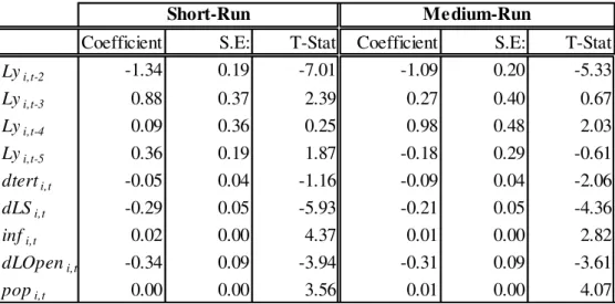
12 Only the two first lags of the lagged per-capita GDP are significant instruments, (see Tables 6 and 7 of the
appendix). Thus, the 2SLS procedure uses two lags of the lagged per capita GDP. Regarding the lagged to-GDP ratio, only one lag is used in the 2SLS procedure, so as to not lose additional observations, since the debt-to-GDP ratio series only starts at 1995. This first lag of the debt-debt-to-GDP ratio is significant (see Table 8 of appendix)
13 Baum et al(2012),
14 The null hypothesis tested implies linearity. See Hansen (2000) for further details in this estimation.
15 Caselli et al (1996) posits that, in panel growth regressions, an adequate strategy to deal with endogeneity is
17
of the same variable. In order to estimate the medium-run model, the observations of the last two years of the sample, i.e. 2013 and 2014, due to the averaging process, were lost.
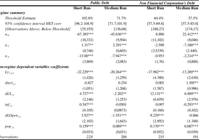
The results conclude in favour of the nonlinear relation between public debt and GDP growth rate. The short run estimation suggests that such threshold occurs around a debt-to-GDP ratio of 103%, above which increases in public indebtedness have a negative effect on growth. This threshold has a 95% significance confidence interval of 96% to 105%. The coefficient of debt in the lower debt-regime (α1)
is positive and significant at a 10% significance level, suggesting that a 1 percentage point increase in debt increases gi,t by 0.01 percentage points, while in the upper debt-regime the coefficient of debt (α2)
is negative and significant at a 5% significance level, suggesting that a 1 percentage point increase in debt decreases gi,t by 0.13 percentage points. The results support the hypothesis of additional public debt
having a positive effect on growth up to a given threshold, above which this effect becomes negative, with a stronger impact in absolute terms.
The medium-run estimation of the public debt specification suggests a lower breakpoint, of 72%, with a less efficient confidence interval of 72% to 102%, statistically significant at a 5% nominal level. The estimated coefficient of α1 in the medium-run has both a higher size and a higher significance than
in the short run, and implies that a 1 percentage point increase in public indebtedness increases GDP growth by 0.02 percentage points, significant at a 5% significance level. On the other hand, the estimated coefficient of α2 is once more negative, despite being lower than in the short run. A 1 percentage point
18 Table 2- Estimation results
Concerning NFC’ indebtedness, the results of the short-run specification are not conclusive
regarding the existence of a threshold effect on the relation of debt with per capita growth rate. A threshold is estimated at 64.4% of indebtedness in the short run, however both α1 and α2 are not
statistically significant, suggesting that the impact of NFC’ debt to GDP ratio is not significant in both regimes.
However, in the medium-run specification, the results provide evidence that an increasing NFC’ debt has always a negative impact on per-capita GDP growth, regardless of its level. Furthermore, the results suggest that this negative impact is more negative below a threshold of 58%, with a confidence interval of 58% to 85% significant at a 5% nominal value, than above this threshold. In the medium-run, if NFC’ debt is below 58% of GDP, a 1 percentage point increase in indebtedness decreases the
output growth by 0.07 percentage points, while if it is above such threshold, a 1 percentage point increase of NFC’ debt-to-GDP ratio leads to a decrease of per-capita GDP growth rate of 0.02 percentage points.
Non Financial Corporation's Debt
Short Run Medium Run Short Run Medium Run
Threshold Estimate 102.8% 71.7% 64.4% 57.5%
95% confidence interval HET corr [96.2-104.9] [71.7;101.9] [57.5-69.8] [57.5-85.0]
[Observations Above; Below Threshold] [35;193] [136;68] [188;27] [174;17]
α0 -67.385*** -45.636*** 8.880 22.412***
(18,332) (9,504) (11,102) (8,046)
α1 1.317** 2.291*** -2.590 -7.100***
(0,746) (0,603) (3,5339) (2.440)
α2 -13.00*** -7.947*** -0.953 -2.214***
(3,869) (2,083) (1,76) (0,888)
Lyi,t-1 -22.229*** -20.264*** -17.982*** -13.269***
(1,426) (1,259) (4.380) (2.630)
dterti,t -0.827 0.254 0.002 1.505**
(1,051) (1,268) (1.587) (0.996)
dLSi,t 4.727*** -2.202** 12.131** 6.889***
(2,146) (1,253) (6.659) (2.976)
infi,t 0.547*** -0.0501 0.097 -0.293***
(0.105) (0,0873) (0.160) (0,102)
dLOpeni,t 3.927** -1.551*** 9.229*** -0.866
(2.102) (1,643) (2.892) (1.348)
popi,t 0.159*** 0.089*** 0.170*** 0.087***
(0.033) (0,031) (0.052) (0.039)
Observations 228 204 215 191
Non-regime dependent variables coefficients Regime summary
19 Table 3- Robustness tests
To test the robustness of these results, further control variables were considered. These variables were i) the age dependency ratio - a measure of the age-structure of societies to control for the ageing European population ii) the terms of trade growth rate – to depict the evolution of the relative competitiveness of countries’ external trade, measured as the price of exports over the price of imports, and iii) the ratio of government consumption to GDP, to capture changes in fiscal policy. Further, regarding NFC’ debt, a series from a different source is used. While the baseline regression used a series published by Eurostat, in this robustness test the source of the NFC’ indebtedness series is the Bank of
International Settlements Statistics database. The previous results are robust to the introduction of further control variables and, regarding NFC’ debt, to the change of the source of data, as summarized in Table 3. However, this robustness does not hold for the short-run impact of public debt on growth in the lower-debt regime, which became insignificant.
Non Financial Corporation's Debt
Short Run Medium Run Short Run Medium Run
Regime summary
Threshold Estimate 102.8% 71.7% 62.9%*** 62.50%
95% confidence interval HET corr [96.6-103.9] [69.9;71.7] [56.1-66.8] [52.6-78.5]
[Observations Above;below threshold] [35;193] [136;68] [46;168] [43;147]
α0 -66.043** -45.848*** 19.715*** 26.101***
(-17,583) (-0,399) (8,156) (6,457)
α1 0.565 2.238*** -6.602 -8.914***
(-0.740) (0,654) (3,208) (2,101)
α2 -12.795*** -8.039*** -2.272 -2.844***
(3,693) (2,068) (1,914) (1,052)
Lyi,t-1 -19.801*** -21.143*** -12.575*** -10.548***
(1.556) (1,379) (5,419) (3,177)
oldagei,t -0.370 0.285 -0.883** -0.353
(0.406) (0,374) (0,503) (0,353)
dterti,t -0.193 0.116 0.155 1.363*
(0.846) (1,277) (1,378) '(0.940)
dLGi,t -7.995 9.002** -31.524*** -15.856***
(8.001) (5,144) (7,537) (4,419)
dLSi,t 5.156*** 3.151*** 5.658*** 3.007***
(2.086) (1.390) (1,831) (1,296)
infi,t 0.450*** -0.014 -0.242** -0.505***
(0.095) (0,086) (0,161) (0,102)
dLOpeni,t 4.322*** -1.657 3.257 -1.059
(2.160) (2,355) (3,191) (2,046)
popi,t 0.122*** 0.089*** 0.131*** 0.074**
(0,03) (0,033) (0,0607) (0.040)
TofTi,t -0.122*** -0.085 -0.335*** -0.107*
(0,045) (0.070) (0,098) (0,071)
Observations 228 204 214 191
Public Debt
20
6.
Discussion of Results
In the 12 euro area countries under study, the results presented above support the hypothesis of a nonlinear relationship between public debt and per-capital GDP growth both in the short and in the medium-run, whereas between NFC’ debt and per-capita GDP growth this nonlinear relationship is only verified in the medium-run alone.
Regarding public indebtedness, the analysis finds evidence against the Ricardian Equivalence hypothesis, since public debt is not neutral in real terms, regardless of its level. Further, it suggests that, for countries in the Eurozone with low and medium levels of public debt, there is a tendency to experience an increase in real growth after an increase in debt. As the revised theoretical literature suggests, these positive impact of public debt may arise, among other reasons, as a result of expansionary fiscal policies that increase households’ disposable income or a smooth of tax revenue. However, once
the public debt threshold is reached, the effect of debt becomes negative, i.e. additional debt build-ups have a negative real impact on the economy. As reviewed in the theoretical literature, this negative impact may arise, among other reasons, as a result of distortionary taxes collected to finance interest payments, a crowding out of total investment or from the increasing likelihood of financial crises. Furthermore, the results indicate that the short-run negative impacts of high and increasing levels of public debt are much more severe than in the medium-run, but while in latter these negative effects are triggered as soon as 72% of indebtedness is reached, in the former these effects are only felt when debt is above 103%.
Concerning NFC’ indebtedness, the results suggest that debt has no impact on the short-run
per-capita GDP growth rate, possibly indicating that entrepreneurs are indifferent between per-capital and debt to finance new projects, providing support for the Modigliani and Miller’s (1958) proposition. However,
this conclusion is no longer adequate in the medium-run, since the results indicate that increases in NFC’ indebtedness have always a negative impact on economic growth. Moreover, this impact becomes less negative when NFC’ debt-to-GDP ratio is above a threshold around 60%, possibly suggesting that
21
In summary, the revised empirical literature on this issue, which either defines or estimates the threshold levels of debt-to-GDP ratio, advances that the breakpoints of the nonlinear relation between public debt and growth assume values between 90% and 100%. Further, it suggests that a 1 percentage point increase of debt-to-GDP ratio in countries in the below-threshold regimes increases growth by a maximum of 0.05 percentage points, and in countries in the above-threshold regime, it decreases growth by a maximum of 0.06 percentage points. Finally, the very scarce literature that assesses the relation of nonfinancial corporations’ indebtedness and growth finds no correlation between the two variables. While the results concerning NFC’ indebtedness are not so analogous, those regarding public debt are
sturdily comparable to this empirical literature. It is so since i) a nonlinear relation of public debt and growth is encountered, ii) in countries with a public debt in the below-threshold regime, an increase in public indebtedness has a positive impact on growth, iii) while in countries with a public debt in the above-threshold regime, an increase in public indebtedness has a depresive real effect on the economy.
Referring to the estimated threshold values of public debt, the short-run estimation, which this research points out to be between 96% and 105%, is comparable to the empirical literature revised, while the medium-run estimation of the debt-to-GDP threshold, 72%, is rather lower than the empirical evidence found in the literature. In addition, the impact of a 1 percentage point increase in debt-to-GDP ratio in the below-threshold regime, which is estimated to be positive and around 0.01 and 0.02 percentage points in the short and in the medium-run, respectively, has a similar magnitude to the results of the empirical researches reviewed. Finally, an analogous increase in debt in countries under the above-threshold regime, which the model predicts to be negative and around 0.13 and 0.08 percentage points in the short and in the medium-run, respectively, is found to be slightly higher than the results of the empirical literature on the issue, suggesting that the negative impact on growth in the euro area of a high and increasing debt is somewhat higher than in other advanced countries, especially in the short-run.
22
Reinhart and Rogoff (2013), revising the historical records of debt overhangs, and mainly focusing on public debt, suggest that advanced economies have, throughout history, made use of five different tracks to reduce national debt: i) economic growth, ii) fiscal adjustment, iii) debts restructurings, iv) inflation surprises and v) a steady dose of financial repression and of inflation. While the official policy approach in the euro area postulates that a constant amount of ii), i.e. austerity, will both bring countries indebtedness to a sustainable path and induce growth, the results of the present research argue in favour of policies that promote an expressive debt reduction. Such policies, as iii), iv) v), aimed at bringing overindebted countries to a low or medium level of indebtedness, induce both an expressive boost to the economy through an increased growth rate, and a recovery of the ability to incur in countercyclical policies without arming growth.
7.
Limitations and areas for further research
Although the discussed results are, in general terms, in accordance with the empirical research on the relation of national debt and growth, some limitations on the methodology applied ought to be considered as a reason to bear these results with caution.
23
insufficient to avoid the reverse causality problem. Hence, a major limitation of this study is that a univocal causal relationship is not totally assured.
Further empirical developments of the analysis ought to overcome, if possible, the limitations mentioned above, notably the adaptation of the methodology to account for additional breakpoints of the debt-to-GDP ratio, the development of a distribution theory for the estimated threshold taking into account possible endogeneity issues and the study of external instrumental variables of debt. Moreover, it is important to address the study of multidimensional debt build-ups, extending the study from government and nonfinancial corporations’ indebtedness to other institutional sectors’ debt.
8.
Conclusion
24
These are very relevant results, and propound that one of the responsible factors for the lethargic growth in the euro area after the financial crisis has been the accumulation of huge stocks of national debt. Notwithstanding the fact that the official policy approach in the euro area is focused on fiscal adjustments to bring countries indebtedness to a sustainable path and induce growth, the results of this research gives room for the discussion of nonconventional policies that promote an expressive debt reduction in over-indebted countries, which stimulates growth and recovers the ability of countries to perform countercyclical policies without harming growth.
9.
Bibliography
Afonso, A., & João, J. (2011). Growth and Productivity: the role of Government Debt. ISEG-UTL, Department of Economics, Working paper no.13/2011/DE/UECE.
Álvarez, I., Barbero, J., & Zofío, J. (2016). A Panel Data Toolbox for Matlab. Journal of Statistical Software.
Ash, M., Herndon, T., & Pollin, R. (2013). Does High Public Debt Consistently Stifle Economic Growth? A Critique of Reinhart and Rogoff. Working Paper Series No. 322 POlitical Economy Research Institute University of Massachussetts Amherst.
Barro, R. (1974). Are Government Bonds Net Wealth. Journal of Political Economy 81: 1095-1117.
Barro, R. (1979). On the determination of the public debt. Journal of Political Economy 87(5): 940-971.
Barro, R. (1990). Government Spending in a Simple Model of Endogenous Growth. Journal of Political Economy, 98: 103-125.
Barro, R., & Sala-i-Martin, X. (2003). Economic Growth. Massachussets: MIT Press.
Baum, A., Checherita-Westphal, C., & Rother, P. (2012). Debt and Growth: New Evidence For the Euro Area. Journal of International Money and Finance, 32: 809–821.
Bernanke, B., & Gertler, M. (1990). Financial Fragility and Economic Performance. The Quarterly Journal of Economics, 105(1): 87–114.
Bick, A. (2010). Threshold effects of inflation on economic growth in developing countries. Econ Lett 108(2):126-129.
Bick, A., Kremer, S., & Nautz, D. (2013). Inflation and Growth: New Evidence From a Dynamic Panel Threshold Analysis.
Empir Econ 44: 861–878.
Buttiglione,, L., Lane, P., Reichlin, L., & Reinhart, V. (2014). Deleveraging, what deleveraging? . 16th Geneva Conference on Managing the World Economy, 9 May, ICMB, CIMB and CEPR, Geneva.
Caner, M., & Hansen, B. (2004). Instrumental Variable Estimation of a Threshold Model. Econom Theory 20: 813–843.
Cecchetti, S., Mohanty, M., & Zampoli, F. (2011). The real effect of debt. BIS Working Papers, no 352.
CHECHERITA, C., & Rother, P. (2012). The Impact of High Government Debt on Economic Growth and its Channels: An Empirical Investigation for the Euro Area. European Economic Review, 56 (7): 1392-1405.
Cochrane , J. (2011). Inflation and Debt. National Affairs, 9: 56–78.
Cukierman, A., & Meltzer, A. (n.d.). A Political Theory of Government Debt and Deficits in a neo-Ricardian Framework.
American Economic Review, 79 (4): 713-732.
25
Diamond, P. (1965). National Debt in a Neoclassical Growth Mode. American Economic Review, 55 (5): 1126-1150.
Eberhardt, M., & Presbitero, A. (2015). Public Debt and Growth: Heterogeneity and non-linearity. Journal of International Economics 97: 45-58.
Effects on a later recall by delaying initial recall. (n.d.).
Égert, B. (2012). Public Debt, Economic Growth and Nonlinear Effects: Myth or Reality? OECD Economics DepartmentWorking Papers 993.
Elmendorf, D., & Mankiw, N. (1998). Government Deb. Board of Governors of the Federal Reserve Finance and Economics Discussion Series, 9.
Financial Instability, the Current Dilemma, and the Structure of Banking. (1977). In H. a. Committee on Banking,
Compendium of Major Issues in Bank Regulation (pp. 310-353). Chicago: U.S. Government Printing Office.
Fisher, I. (1933). The Debt-Deflation Theory of Great Depressions. .Econometrica, 1: 337-57.
Geanakoplos, J. (2009). Leverage Cycles. NBER Macroeconomics Annual, 24: 1–65.
Greiner , A. (2013). Public Debt, Productive Public Spending and Endogenous Growth. Bielefeld Working Papers in Economics and Management, 23.
Hansen, B. (1999). Threshold Effects in Non-Dynamic Panels: Estimation, testing and inference. Journal of Econometrics 93: 345-368.
Hausman, J. (1979). Specification Tests in Econometrics. Econometrica,46,:1251-1271.
Hausman, R., & Panizza, U. (.2011.). Redemption or Abstinence? Original Sin, Currency Mismatches, and Counter Cyclcial Policies in the New Millenium. Jornal of Globalization and Development 2(1): 1-35.
Im, K., Pesaran, M., & Shin, Y. (2003). Testing for unit roots in heterogeneous panels. Journal of Econometrics, 115_ 53-74.
Islam, N. (1995). Growth Empirics: A Panel Data Approach. Quarterly Journal of Economics, 110: 1127-1170.
Keynes, J. (1930). A Treatise on Money. London: Macmillan.
Kindleberger, C. (1978). Manias, Panics and Crashes. New York: Wiley.
Krugman, P. (1988). Financing versus Forgiving a Debt Overhang. Working Paper No. 2486 , NBER, Cambridge, MA.
Kumar, M., & Woo, J. (2010). Public Debt and Growth. IMF Working Paper WP/10/174.
Kydland, F., & Prescott, E. (1978). On the feasibility and desirability of stabilization policy. In S. Fischer, Rational expectations and economic policy. Chicago, : University of Chicago Press for National Bureau of Economic Research.
Levin, A., Lin, C., & Chu, C. (2002). Unit root test in panel data: Asymptotic and finite sample properties. Journal of Econometrics, 108:1-22.
Lindert, P., & Morton, P. (1989). How Sovereign Debt. In J. D. Sachs, Developing Country Debt and Economic Performance, Volume (pp. 39-106). University of Chicago Press.
Maddala, G., & Wu, S. (1999). A comparative study of unit root tests with panel data and new simple test. Oxford Bullertin of Economics and Statistics, Speccial issue: 631-652.
Marx, K. (1862). Capital: A Critique of Political Economy. London: Penguin .
Minea, A., & Parent, A. (2012). Is High Public Debt Always Harmful to Economic Growth? Reinhart and Rogoff and some complex nonlinearities. CERDI, Etudes et Documents, E 2012.18.
Minsky, H. (1992). The Financial Instability Hypothesis. Working paper no. 74, The Jerome Levy Economics Institute of Bard College.
26
Modigliani, F. (1998). “The Role of Intergenerational Transfers and Life-Cycle Saving in the Accumulation of Wealth. Journal of Economic Perspectives, 2(2): 15–20.
Modigliani, F., & Miller, M. (1958). The Cost of Capital, Corporation Finance, and the Theory of Investment. American Economic Review, 48: 267-297.
Panizza, U., & Presbitero, A. (2013). Public debt and economic growth in advanced economies: a survey. Swiss J. Econ. Stat. 149 (2), 175–204.
Panizza, U., & Presbitero, A. F. (2014). Public Debt and Economic Growth: Is there a causal effect? Journal of Macroeconometrics 41: 21-41.
Patillo, C., Poirson, H., & Ricci, L. (2011). MoFiR Working Paper. No. 78. MoFiR Working Paper. No. 78, 2 (3).
Ramey, G., & Ramey, V. (.1995). Cross-Country Evidence on the Link Between Volatility and Growth. .American Economic Review, 85(5): 1138–51.
Reinhart, C. a. (2010.). Growth in a Time of Debt. .American Economic Review, 100(2): 573–78.
Reinhart, C., Reinhart, V., & Rogoff, K. (n.d.). Public Debt Ovehangs: Advanced-Economy Episodes Since 1800. Journal of Economic Perspectives, 26 (3): 69-86.
Ricardo, D. (1817). Principles of Political Economy and Taxation. London: Dent.
Saint-Paul, G. (1992). Fiscal Policy in an Endogenous Growth Model. Quarterly Journal of Economics, 107: 1243-1259.
Sala-i-Martin, X., Doppelhofer, G., & Miller, R. (2004). Determinants of Long-Term Growth: A Bayesian averaging of classical estimates (BACE) approach . American Economic Review.94:813-835.
Schularick, M., & Taylor, M. (2009). Credit Booms Gone Bust: Monetary Policy, Leverage Cycles and Financial Crises.
Working Paper no. 15512, NBER, Cambridge, MA.
27
10.
Appendix
Graph 1 - Evolution of public debt-to-GDP ratio and per-capita GDP growth rate, average of 12 euro area countries
28
29 Table 4 - Details of the constructed database
Variable Periods Source Observations
Public debt 1995-2015 AMECO Values of public debt as defined by the Maastricht Treaty
EUROSTAT
Values of NFC' debt , including (F2)Currency and Deposits, (F3) Debt Securities, (F4) Loans, (F6)Insurance, Pension Funds and Standardized Guarantee Schemes and (F8) Other account receivable/payable
BIS Values of NFC' debt includes (F3) Debt Securities and (F4) Loans
Per-Capita Real GDP 1990-2015 AMECO The series was extended back to 1990 in order to perform the 2SLS without loosing observations
Age-Dependency Ratio 1995-2015 EUROSTAT
School Life Expectancy in Tertiary
Education 1995-2015 ONU / EUROSTAT
Obtained by filling the missing values of the series of EUROSTAT with the values of the series of ONU, summed with the average differences between them
Government Final Consumption 1995-2015 AMECO/EUROSTAT
Obtained by filling the missing values of the series of AMECO with the values of the series of EUROSTAT, summed with the average differences between them
Total Gross Savings 1995-2015 AMECO
Inflation 1995-2015 OECD
Openness 1995-2015 AMECO
Population Growth Rate 1995-2015 EUROSTAT
Terms of Trade Growth Rate 1995-2015 AMECO
30 Table 5 - Hausman Test’s Results
Table 6 – Lagged Per-capita GDP 2SLS procedure with 4 lags
Table 7 – Lagged Per-capita GDP 2SLS procedure with 4 lags
A: FE2SLS B: RE2SLS Coef. Diff S.E. Diff
Lpubdebt 9.86 7.63 2.22 1.14
Oldage -0.37 -0.29 -0.09 0.12
Tertiary 1.11 -0.59 1.70 0.53
G -0.13 0.65 0.53 0.20
GRSTot 0.80 0.48 0.32 0.09
Inf 0.05 -0.09 0.15 0.00
Openn -0.05 0.00 -0.05 0.02
PopGr 0.18 0.17 0.02 0.00
TofTr -0.02 -0.02 0.00 0.00
A is consistent under H0 and H1 (A = FE2SLS) B is consistent under H0 (B = RE2SLS) H0: coef(A) - coef(B) = 0 H = 101.394285 ~ Chi2(9)
H1: coef(A) - coef(B) ≠ 0 p-value = 0.0000
Coefficient S.E: T-Stat Coefficient S.E: T-Stat
Lyi,t-2 -1.34 0.19 -7.01 -1.09 0.20 -5.33
Lyi,t-3 0.88 0.37 2.39 0.27 0.40 0.67
Lyi,t-4 0.09 0.36 0.25 0.98 0.48 2.03
Lyi,t-5 0.36 0.19 1.87 -0.18 0.29 -0.61
dterti,t -0.05 0.04 -1.16 -0.09 0.04 -2.06
dLSi,t -0.29 0.05 -5.93 -0.21 0.05 -4.36
infi,t 0.02 0.00 4.37 0.01 0.00 2.82
dLOpeni,t -0.34 0.09 -3.94 -0.31 0.09 -3.61
popi,t 0.00 0.00 3.56 0.01 0.00 4.07
Short-Run Medium-Run
Coefficient S.E: T-Stat Coefficient S.E: T-Stat
Lyi,t-2 -1.67 0.16 -10.53 -1.48 0.17 -8.55
Lyi,t-3 1.66 0.16 10.42 1.47 0.17 8.43
dterti,t -0.05 0.04 -1.16 -0.09 0.04 -2.02
dLSi,t -0.29 0.05 -5.93 -0.21 0.05 -4.14
infi,t 0.02 0.00 5.05 0.02 0.00 3.78
dLOpeni,t -0.31 0.09 -3.47 -0.30 0.09 -3.39
popi,t 0.00 0.00 3.14 0.01 0.00 3.94
31 Table 8- Lagged Debt-to-GDP 2SLS procedure with 1 lag
Coefficient S.E: T-Stat
Ldi,t-2 -0.02 0.00 -6.53
dterti,t 0.15 0.13 1.22
dLSi,t 0.57 0.16 3.63
infi,t -0.01 0.01 -0.48
dLOpeni,t 0.05 0.28 0.17