The use of Pedotransfer functions and the estimation of carbon stock in the Central

ABSTRACT: Computer models have been used to assess soil organic carbon (SOC) stock change. Commonly, models require to determine soil bulk density (Db), a variable that is often

lacking in soil data bases. To partly overcome this problem, pedotransfer functions (PTFs) are developed to estimate Db from other easily available soil properties. However, only a few studies

have determined the accuracy of these functions and quantified their effects on the final quality of the spatial variability maps. In this context, the objectives of this study were: i) to develop one PTF to estimate Dbin soils of the Brazilian Central Amazon region; ii) to compare the

per-formance of PTFs generated with three other models generally used to estimate Dbin soils of

the Amazon region; and iii) to quantify the effect of applying these PTFs on the spatial variability maps of SOC stock. Using data from 96 soil profiles in the Urucu river basin in Brazil, a multiple linear regression model was generated to estimate D_b using SOC, pH, sum of basic cations, aluminum (Al+3_{), and clay content. This model outperformed the three other PTFs published in} the literature. The average estimation error of SOC stock using our model was 0.03 Mg C ha−1_, which is markedly lower than the other PTFs (1.06 and 1.23 Mg C ha−1_{, or 15 % and 17 %,} respectively). Thus, the application of a non-validated PTF to estimate D_b can introduce an error that is large enough to skew the significant difference in soil carbon stock change.

Keywords: Içá Formation, multiple linear regression, ordinary kriging

The use of Pedotransfer functions and the estimation of carbon stock in the Central

Andréa da Silva Gomes1_{, Ana Carolina de Souza Ferreira}1_{, Érika Flávia Machado Pinheiro}1_{, Michele Duarte de Menezes}2_{, Marcos}

Bacis Ceddia1_*

1_{Federal Rural University of Rio de Janeiro/Institute of} Agronomy – Dept. of Soil, BR-465, km 7 − 23897-000 − Seropédica, RJ − Brazil.

2_{Federal University of Lavras – Dept. of Soil Science, C.P.} 3037 − 37200-000 − Lavras, MG − Brazil.

*Corresponding author <marcosceddia@gmail.com>

Edited by: Francesco Montemurro

Received August 04, 2016 Accepted November 18, 2016

Introduction

Pedotransfer functions (PTFs) are predictive mod-els of certain soil properties using data from soil surveys (Bouma, 1989). These functions fill the gap between the available soil data and the properties that are more use-ful or required for a particular model or quality assess-ment. In this work, PTFs are used as

physical-mathe-matical models that allow the estimation of D_b from soil

data, which are needed to convert carbon contents from percentage of dry weight to carbon mass per unit of area (Howard et al., 1995; Benites et al., 2007).

The lack of D_b data is a limiting factor in regions

such as the Brazilian Amazon. With a few exceptions, the lack of detailed maps along the region is partly due to: a) accessibility (often only possible by boat or airplane), b) a vast territory extension is covered by the Tropical Amazon Forest, and c) lack of more detailed ancillary maps, including topographic, geologic, and geomorphologic maps. Bernoux et al. (1998) and Tomasella and Hodnett (1998)

provided the first baseline to predict D_b from databases.

These authors used data from the RADAMBRASIL project (RADAMBRASIL, 1978). More recently, Benites et al. (2007) used data from the Soil Archives of Embrapa (Brazilian Corporation of Agriculture Research) to develop

a PTF to estimate D_b for most Brazilian biomes. These

three PTFs are frequently applied to predict D_b of soils in

Brazil (Bernoux et al., 2002).

Typically, PTF-estimated attributes are used di-rectly in numerical modeling, although the accuracy of the attribute estimates and their effect on modeling

results are not often investigated or they are simply ig-nored (Deng et al., 2009). Despite the importance of these SOC stock estimations for Brazilian soils in the Amazon region, it is important to highlight that most

studies that have applied the PTFs above to estimate D_b

do not present quantitative information about the error caused by the application of these PTFs. Bernoux et

al. (1998), reported that D_b estimation using their PTF

could lead to an error of ≤ 10 % in the final calculation

of carbon stock (CS) in 323 horizons used in the study. In this context, the purpose of this study was to

predict D_b from readily available soil properties of Içá

Formation in the Brazilian Amazon region, considering the minor effort and uncertainty principles. We have also compared the performance of the models gener-ated in this study with those in the literature (Bernoux et al., 1998; Tomasella and Hodnett, 1998; Benites et al., 2007). Finally, we quantified the error due the

ap-plication of different PTFs to estimate D_b in the spatial

variability of soil carbon stock.

Materials and Methods

Study site, soils, and the database

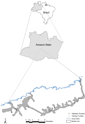
The study site is located in the central region of the Amazon State near the Urucu River in the munici-pality of Coari, Brazil, more specifically between the geographic coordinates 4º 45’S and 65º 25’W and the average elevation is 60 m above the sea level (Figure 1). The region is located about 640 km from the state capital Manaus, and it can only be accessed by boat

or airplane. The climate is equatorial (Af-Köppen Cli-mate Classification) where the temperature in the cold-est month is higher than 20 °C, with no pronounced dry period and a mean annual precipitation of 2500 mm.

The sampled area covers about 80 km2_{, spanning}

longitudinally across the IçáGeologic Formation, which

is part of the Solimões Geologic Domain. The soils of the

study site were formed from sediments of Içá Geologic Formation (RADAMBRASIL, 1978). The Içá Formation consists of fine to medium sandstone and siltstone with clay conglomerates and yellow-red. The Holocene allu-vium of the Quaternary Period deposits is related to the current Amazonian drainage networks. The sediments

of Içá Formation cover an area of 563,264 km2 _{(36 % of}

the Amazon State) and were deposited in the Tertiary-Quaternary Period.

A soil survey was conducted in the Oil Province of Urucu River (named Geólogo Pedro de Moura) between the years of 2008 and 2009. This work resulted in the generation of a soil map along with its respective report

(Ceddia et al., 2015), which covers an area of 79.665 km2

(Figure 1). Throughout the soil survey, 96 soil profiles

were described and sampled by horizon, totaling 483 horizons/samples. Due to the limitations imposed by the native vegetation, the 315 field observations were restricted to the vicinity of access roads and only data from 96 soil profiles were used for this study.

The soils were classified based on the Brazilian Soil Classification System (Embrapa, 1999). The soil-mapping units of the study site as well as the number of profiles and area of occurrence are shown in Table 1.

In each horizon of the 96 soil profiles, disturbed soil samples were taken for the following soil chemical attributes: pH (water), Ca+2_{, Mg}+2_{, K}+_{, Na}+_{, Al}3+_{, H}+_, P, CEC, SB (sum of basic cations), V value (base

satura-tion) and Al3+ _{saturation. The soil chemical analysis was}

performed according to Embrapa (1997). SOC was mea-sured by wet combustion (Walkley and Black, 1932). Soil physical data consisted of particle size measurements, comprising sand (2.00-0.05 mm), silt (0.05-0.002 mm) and clay (< 0.002 mm) by the Pipette method.

Undisturbed soil sampling for D_b was done by the

core method using standard steel cylinders of 53 cm3

volume (h = 42 mm, d = 40 mm). In each of the 96 soil

profiles, the steel cylinders were inserted into the cen-ter of each soil horizon (perpendicular to the surface). The soil-filled cylinder was carefully removed from the ring holder and the soil extending beyond both cylinder ends was trimmed flush using a sharp knife. Protective plastic covers were used to prevent samples from drying out. The samples were transported to the laboratory and were oven dried (105 °C) until constant weight (24-48 h).

Development of the pedotransfer function

The first step in the PTFs generation was the selec-tion of the model development (training) and validaselec-tion of the dataset. The 96 soil profiles were randomly split (80/20) into training and validation sets. Thus, the data-set used for training consisted of 77 soil profiles (adding up to 378 horizons), while the dataset used for validation consisted of 19 soil profiles (adding up to 105 horizons). The spatial distribution of the training and validation soil profiles along the study area are presented in Figure 1.

The stepwise multiple regression routine was used

for explanatory analysis relating D_b to soils attributes.

The Akaike Information Criterion (AIC) with a p-value

of 0.05 was used to include or exclude variables. All linear model assumptions were checked

(multicollinear-Table 1 − Distribution of soil class in the data set.

Order

(Embrapa, 1999) (FAO, 1998)FAO-WRB Number of soil profiles Total %

Argissolos Acrisols, Lixisols 53 55

Cambissolos Cambisols 39 41

Espodossolo Spodosol 1 1

Neossolos Arenosols, Fluvisols 2 2

Planossolo Planosol 1 1

Total 96 100

ity, homoscedasticity and the normality of regression residues). Multicollinearity was minimized by removing variables with variance inflation factors > 4. To veri-fy the premise of homoscedasticity was performed the Breusch-Pagan test and regression normality residues was performed by the Kolmogorov-Smirnov (KS). The stepwise regression was performed by the R software (R Development Core Team, version 3.1.1).

The explanatory analysis was conducted consid-ering two possibilities: a) construction of a unique re-gression model to estimate soil bulk density for all soil depths, and b) construction of two regression models, one for surface horizons (A and AB) and another for subsurface horizons (BA, B, BC, C). The final choice of the model to be used was based on the evaluation of

the indices AIC, R2 _{and standard error (SE) of the}

step-wise regression. Therefore, the best model presented the

highest R2 _{and the lowest SE and AIC.}

The evaluation of the pedotransfer function perfor-mance

This study compares the applicability of the proposed multiple regression model with three existing models in the literature (Bernoux et al., 1998; Tomasella and Hodnett, 1998; Benites et al., 2007), which are presented in Table 2.

We simulated a situation where the database of the

study area lacked D_b data. Thus, to estimate the carbon

stock, it would be necessary to use a pedotransfer function

available in the literature. Commonly, when D_b data are not

available in soils of the Amazon region, researchers choose one of these three PTFs, although the criteria to choose a specific PTF is subjective and not clearly explained. Bernoux et al. (1998) and Tomasella and Hodnett (1998)

generated the first two PTFs to predict D_b data from

properties for soil across the Amazon basin and both used the soil data set generated by the RADAMBRASIL project (RADAMBRASIL, 1978). More recently, Benites et al. (2007)

generated a model to predict D_b from readily available soil

properties of Brazilian soils found in most biomes. The latter study constructed a database from the Soil Archives of Embrapa Solos in Rio de Janeiro, Brazil.

The predicted values (yi) of D_b, using different

PTFs were compared with the 104 observed values (ŷi)

in the validation dataset. The differences between the

104 predicted and observed values (ŷ_i – y_i) were used to

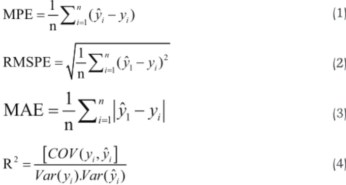
calculate the following error measurements: the mean prediction error (MPE), Eq. (1); the root mean squared prediction error (RMSPE), Eq. (2); the mean absolute error (MAE), Eq. (3); and the prediction coefficient

of determination (R2_{), Eq. (4). The results were also}

evaluated graphically by the ratio 1:1 of the observed vs

predicted values.

1

1 ˆ

MPE ( )

n n

i i

i= y y

=

_∑

RMSPE ( )

n n

i i= y y

=

_∑

1 1

1

ˆ

MAE

n

y

y

=

∑

−

[

]

2 ( ,ˆ

R

ˆ ( ). ( )

i i

i i

COV y y

Var y Var y

= (4)

where: ŷ_i is observed D_b of ith soil sample; y_i is predicted

D_b of ith soil sample, and n is total number of observations. The MPE (accuracy error) enables the evaluation of an average tendency for overestimation (positive values) or underestimation (negative values). The closer to zero MPE is, the greater the model accuracy. MAE is an accu-racy indicator, but it does not reveal the trend to over- or underestimation. This is because it uses an absolute value because of the difference between the observed and pre-dicted data. The RMSPE should be zero, when a perfect fit between the observed and predicted data is achieved.

Spatial variability map of soil organic carbon stock

using measured and estimated values of D

b by PTFs For each of the 96 soil profiles, the calculation of the SOC stock was performed at 0-100 cm depth. The clas-sical way of calculating SOC stock (C mass per area) for a given depth consists of summing C stocks by horizon,

determined as a product of D_b, SOC content, and horizon

thickness (Eq.5), according to Bernoux et al. (2002):

SOC stock = (SOC × D_b × T) (5)

where: SOC stock is soil organic carbon stock (kg C m−2_);

SOC is soil organic carbon (g kg−1_{); D}

b is the soil bulk

density (Mg m−3_{) and, T is the horizon thickness (m).}

Table 2 − Soil bulk density estimate models from the literature (Benites et al., 2007).

Regression models

(Region) Nsp Nh

Data density

sp/km2 Equations

Bernoux et al. (1998)

(B.L.A.- 5,020,000 km2₎ 690 323 0.00014 Db = 1.524 – 0.0038 (% clay) – 0.050 (%SOC) – 0.045 (pHH2O) + 0,001 (% sand) Tomasella and Hodnett (1998)

(B.L.A.- 5,020,000 km2₎ 1162 396 0.00023 Db = 1.578 – 0.054 (% SOC) – 0.006 (% silt) – 0.004 (% clay)

Benites et al. (2007)

(M.B.B - 8,516,000 km2₎ 363 1542 0.00007 Db = 1.560 – 0.0005 (g kg−1 clay) – 0.010 (g kg−1 SOC) + 0.0075 (SB)

B.L.A. = Brazilian Legal Amazon Region; M.B.B. = Most Brazilian Biomes (Brazilian Territory); Nsp = number of soil profiles; Nh = number of soil horizons/layers with D_bdata; Data Density (sp/km2_{) = Number of soil profiles per square kilometers; D}

In the soil survey, the soil profiles were divided into horizons (A, B, and C). In most cases, the calculations concerned two horizons where the first horizon was typically entirely above 100 cm, and the second one crossed this 100 cm depth. When a horizon crossed the 100 cm boundary, only the horizon portion above that depth was used to calculate its SOC stock.

Considering the measured data_, as well as the

four estimates of D_b (model generated in this work

and three other published in the literature (Bernoux et al., 1998; Tomasella and Hodnett, 1998; Benites et al., 2007), a total of five dataset of SOC stocks at the layers 0-100 cm depth were generated. For each of the five dataset of SOC stocks, experimental semivariograms were calculated for spatial dependence evaluation and a theoretical model that best represented the data variability was set. The experimental semivariogram,

g(h), of n spatial observations Z(xi), i = 1, ... n, was

calculated using equation 6:

g( ) ( )

( )

h

N h i Zxi Zxi h N h −

[

]

∑

where: N(h) = the number of observations separated

by distance h; Z_xi = the soil attribute value measured at

a specific point (x₁) of the grid; Z_xi+h= the soil attribute value measured at a specific neighbor point apart by distance h (xi+h).

The theoretical model was validated by the Jack-knife tool (self-validation or cross-validation). Thereafter, five spatial variability maps of SOC stocks were generated by the ordinary kriging (OK) method. OK only uses primary data such as SOC stocks

measured at sampled locations u to estimate SOC

stocks at unsampled locations (Wackernagel, 2003). For the study site, SOC stock is the primary variable

Z_i (u), measured at sampled locations u to estimate

SOC stocks at unsampled locations (ZOKu

* _{( )). The}

stationarity of the mean is assumed only within a local

neighborhood W(u), centered at the location u being

estimated. Here, the mean is deemed to be a constant but unknown value, i.e., m(u´)=constant but unknown,

∀u´∈ W(u). The OK estimator (Eq. 7) is written as a

linear combination of the n(u) data Z_i(u) with a single

unbiasedness constraint (Eq. 8), as below:

ZOK u Z u

n u

i

*

( )

( )

( )

 

=

∑

α

α1 (7)

with n u_λOK

α

α= =

∑

The unknown local mean m(u) is filtered from the

linear estimator by forcing the kriging weights (l) to sum

to 1 (Eq. 8). The weights l are chosen so that the estimate

ZOKu

* _{( )}

is unbiased, and that the estimation variance

σOK u(0)

2 _{(Eq. 9) is less than any other linear combination of}

the observed values. The minimum variance of ZOKu

* _{( )}

is given by:

σOK u i λ γα µ

N i u u, 0

2

1 0

( )=

∑

(

)

and is obtained when

λ γα µ γ

i N

i j i

u u u u

=

∑

(

)

(

)

where: g(u_i, u_j) = the semivariance of z between the sam-pling points u_i and u_j; g(u₁, u₀) = the semivariance of z

between the sampling point u_i and the unvisited point

u₀; Both quantities g(u_i, u_j) and g(u₁, u₀) are obtained from the theoretical model fitted to the experimental semivar-iogram; µ = the Langrange multiplier required for the minimization.

The semivariogram calculation, Jack-knife and ordinary kriging procedures were conducted using the software Geoestat (Vieira at al., 1983). The kriged files were exported to software ArcGIS (ESRI, version 9.3), where the spatial variability maps of SOC were made.

The evaluation of the spatial variability error of SOC stock from measured and estimated values of

D

b by PTFs

In order to compare the maps generated from

dif-ferent data of D_b, spatial analysis through map algebra

(ArcGIS Raster Calculator Function) was performed. The spatial variability map of carbon stocks generated from the measured data (96 SOC stock values using

mea-sured values of carbon content and D_b) was considered

the most appropriate map (reference map). Then, we calculated how much of each PTF used to estimate the

D_b would over- or underestimate the soil carbon stock.

This procedure allowed determining the carbon stock residual (up to 1 m) from the use of each PTF. The re-siduals were calculated subtracting (pixel by pixel) the carbon stock values in the reference map, in relation to the others generated from the application of PTFs. For this study, each pixel has an area of 1 ha (resolution of 100 by 100 m).

Results and Discussion

Descriptive statistics and the correlation between

D

b and other soil attributes

Descriptive statistics of soil properties are shown in Table 3. The 483 soil horizons covered a wide range of soil textural classes, although sandy and franco silty were the most predominant classes. We highlight the relatively high silt content (mean value of 339, reaching

up to 721 g kg−1_{), since this granulometric fraction is not}

commonly higher than 200 g kg−1 _{in the main classes}

of Brazilian soils. However, along the Central Amazon Region, the soils are formed over sediments of Içá and Solimões formations (consisted of fine to medium sand-stone and siltsand-stone). High values of silt were already re-ported by Tomasella and Hodnett (1998). The authors found silt values in their dataset that reached up to 800

Içá Formation, as well as the type and diversity of veg-etation and consequently the carbon supply to the soil (RADAMBRASIL, 1978; Ceddia et al., 2015). The

coef-ficient of variation for D_b was 16 %, slightly higher than

that previously reported for the Amazon Basin (Moraes et al., 1995; Bernoux et al., 1998). Moraes et al. (1995) observed CV values of 7 % for Alfisols and Ultisols and 13 % for Oxisols, whereas others (Bernoux et al., 1998) have reported a CV of 10 % and 11 % for Oxisols and Alfisols and Ultisols, respectively.

The regression model generated and the compari-son with previously published models

The results of the stepwise analysis to select the

regression models and respective predictors for D_b for

all soil depths, as well as for the surface and sub surface horizons, are presented in Table 4. All models generated showed a normal distribution of the regression residu-als (Kolmogorov-Smirnov test). With the exception of the regression model for soil surface layer, the models (all horizons and subsurface) fulfilled the homoscedasticity premise as confirmed by the Breusch-Pagan test (Table 4).

The D_b varies according to soil depth (Harrison

and Bocock, 1981; Leonaviciute, 2000) however, our results show no improvement in the prediction capac-ity of the models after doing a separate calibration of superficial horizons from the sub-superficial horizons. Similarly, De Vos et al. (2005) did not find any significant enhancement in the predictive capacity when datasets from top and subsoil layers in forest soils of the Flanders region (Belgium) were separated. Other authors working with different regions in the world, such as Han et al. (2012) in China, Sequeira et al. (2014) and Heuscher et al. (2005) in the United States, also did not find any

im-provement in the prediction of D_b generating separated

regression model for surface and subsurface soil layers. The PTFs published in the literature, which are recom-mended to be applied to the Amazon region (Bernoux et al., 1998; Tomasella and Hodnett, 1998) and to most Brazilian biomes (Benites et al., 2007), are used for all soil depths. However, more recently the performance of models was evaluated in soils of most Brazilian biomes presented high acidity and aluminum toxicity and low

sum of basis (SB). As characteristics of the study site, the

mean Al+3 _{content was 4.03 cmol}

c dm

−3 _{(ranging from}

0.25 to 12.00 cmol_c dm−3_{). All chemical properties,}

ex-cept for pH measurements, had a CV > 45 %. The SOC

contents ranged from 0.10 to 60.30 g kg−1 _{and a CV of}

74 %.

The skewness and kurtosis coefficient could be used to infer about the normal data distribution (sym-metric histogram). A zero value for both coefficients means that the attribute presents a normal distribution. Although there is no clear-cut guidelines, most studies consider data to be approximately normal in shape if the skewness and the kurtosis values range from -1.0 to +1.0 (Huck, 2012). Considering this range for skewness

and kurtosis, with the exception of H+ _{and SOC content,}

all soil properties follow within a normal distribution.

The mean D_b measured was 1.25 Mg m−3_{, with}

minimum and maximum values of 0.49 and 1.67 Mg

m−3_{, respectively. The lowest D}

b value is due to the high-est amount of soil organic matter (SOM) in well drained

soils (complex CXa1-typic dystrudepets and PVAa-

typichap-ludults) as opposed to poorly drained soils (consociation

PACd- typicendoaquults) in the Amazon Forest (Ceddia et

al., 2015). The relief is considered the main factor influ-encing the variability of soil types and their attributes in

Table 3 − Descriptive statistics of the soil properties.

Soil property Mean Min. Max. SD CV Skewness Kurtosis D_b(Mg m−3_{) 1.25 0.49 1.67 0.20 16 -0.76 0.44} Sand (g kg−1_{) 393 22 918 173.70 44 0.52 0.002} Silt (g kg−1_{) 339 26 721 122.58 36 0.11 0.04} Clay (g kg−1_{) 266 13 640 131.06 49 0.21 -0.65}

pH_H2O 4.58 3.50 5.70 0.39 8 -0.07 -0.29

SB (cmol_c dm−3_{) 1.65 0.30 4.52 0.87 52 0.70 -0.45} Al3+ _(cmol

c dm−3) 4.03 0.25 9.50 1.84 45 0.31 -0.25 H+ _(cmol

c dm−3) 3.64 0.05 21.70 3.41 94 2.15 5.35 SOC (g kg−1_{) 7.29 0.10 31.68 5.46 74 1.74 3.59} Min. = minimum; Max. = maximum; SD = standard deviation; CV = coefficient of variation (%); D_b = soil bulk density; SOC = soil organic carbon; SB = sum of basic cations.

Table 4 − Candidate models to predict soil bulk density for all soil depth and dividing the dataset into surface and subsurface horizons.

Models (All soil depth) Int. SOC pH_H2O SB Al3+ _{Clay Silt Sand AIC SE R}2 _{KS (p value) BP (p value)}

1 1.171 -0.0237 0.0622 -0.0230 -0.0124 0.0002 -1593.53 0.1205 0.6672 0.6303 0.2566

VIF - 1.75 1.50 1.57 2.57 2.87

Models (Surface) Int. SOC pH_H2O SB Silt Sand Clay Al3+ _{AIC SE R}2 _{KS (p value) BP (p value)}

2 0.609 -0.015 0.145 -546.08 0.1427 0.4745 0.7751 0.0238

VIF - 1.05 1.05

Models (Subsurface) Int. SOC Silt Clay Al3+ _pH

H2O Sand SB SE R2 KS (p value) BP (p value)

3 1.419 -0.029 0.0002 -1049.72 0.1167 0.2474 0.8385 0.0621

VIF - 1.00 1.00

after separation for surface (to 30 cm depth) and sub-surface (below 30 cm) (Benites et al., 2007). The authors did not found any advantage of partitioning the dataset into groups of soil depth and soil orders (Benites et al., 2007). Here, we highlight the model number 1 in Table 4 (Eq. 11) that could be used for all soil depths. This model explained 67 % of the variance and presented the lowest

value of AIC and the highest value of R2_{. The SOC was}

the main predicted variable followed by pH_H2O, SB, Al+3

andClay.

D_b = 1.171 - 0.0237(SOC) + 0.0622(pH) - 0.0230(SB) -

0.0124(Al+3_{) + 0.0002(Clay) (11)}

Consistent with the findings of many authors, SOM clearly plays a dominant role (Adams, 1973; De Vos et al., 2005; Heuschek et al., 2005; Han et al., 2012) because of its much lower density than mineral soil

par-ticles and its aggregation effect on soil structure. The D_b

strongly correlates with SOM content and soil texture

(Adams, 1973; Manrique and Jones, 1991). Barros and

Fearnside (2015), working with oxisoils, also in the Cen-tral Amazon region, found that the clay content accounts for about 70 % of the variation in soil bulk density.

How-ever, the importance of each variable depends on the

study site. For example,De Vos et al. (2005) found that

the addition of texture as a predictor has a minor effect

on D_b estimation of forest soils. In fact, the authors

ob-served that SOM accounted for 55 to 57 % of the total

variation in D_b, whereas soil texture explained only 20

to 26 %.

In the literature, the relationship between D_b and

chemical attributes (such as pH, SB and Al+3_{) is scarcely}

reported and a direct physical link is not clearly pre-sented. In most cases, these attributes are inserted into the model due to their availability in most datasets, be-cause chemical attributes are determined at low costs (Bernoux et al., 1998). For instance, Bernoux et al. (1998) used pH in water and Benites et al. (2007) used SB to

estimate D_b. However, these authors did not provide a

physical explanation regarding the relationship between

either pH or SB with D_b. In tropical soils, the main clay

minerals are kaolinite, goethite, hematite and gibbsite, which are colloids with variable charges depending on the pH. The main clay minerals in the study site are kaolinite and goethite, consequently, as the pH is very low (4.58 on average) and organic colloids are mainly responsible for the CEC of the soil, cation bridges are

formed between soil particles. Cation flocculants (Al+3_,

Fe+3 _{and H}+_{) promote the approximation of the}

colloi-dal particles, which is the first step for the aggregation formation. The next step of aggregate formation is ce-mentation, where SOC has an important role, acting as an agent that cements flocculated particles (Tisdall and Oades, 1982). Finally, soil macro-aggregates are formed, which improves the soil porosity and consequently

re-duces D_b. In uncultivated soils, like most forest soils, the

OM has a dominant effect over D_b (Adams, 1973) and,

naturally, becomes the main predictor variable (De Vos et al., 2005). Considering that the main colloids of the study site in charges that depend on the pH, we

hypoth-esize that Al+3 _{and H}+ _{availability increases as the pH is}

lowered. Therefore, colloids flocculate and increase soil porosity and decrease soil bulk density.

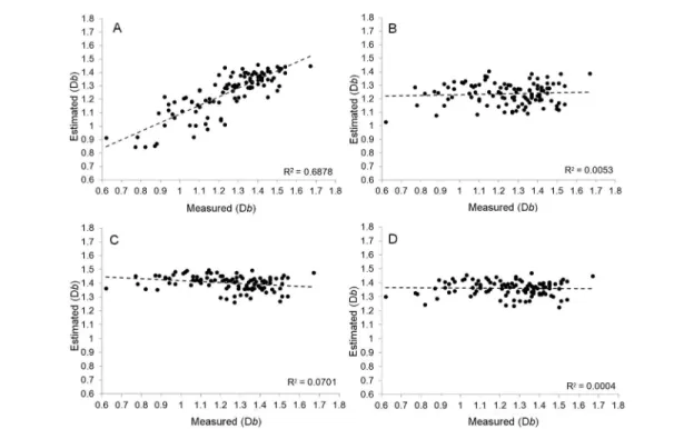
Compared to other PTFs, the proposed model (Eq.11) presented the best agreement (Figures 2A, B, C and D). Considering the MPE index, our proposed mod-el presented the lowest bias, once it reached the ideal value (MPE = 0). The model proposed by Tomasella

and Hodnett (1998) tended to underestimate D_b (MPE

= -0.03 kg dm−3_{), whereas the models by Benites et al.}

(2007) and by Bernoux et al. (1998) tended to

overesti-mate D_b (0.11 and 0.15kg dm−3_{, respectively). The MAE}

value ranged between 0.09 and 0.19 kg dm−3_{, and the}

highest value was observed in the Bernoux et al. (1998) model, followed by the Tomasella and Hodnett (1998) and the Benites et al. (2007) models. The Bernoux et al. (1998) model presented the highest RMSPE value and our model the lowest (Table 5). Barros and Fearnside (2015) also developed PTFs for Oxisols in the Central Amazon region and compared the performance of their model with those presented by authors reported in this work (Benites et al., 2007; Bernoux et al., 1998; Toma-sella and Hodnett, 1998). The authors found that the application of these three PTFs overestimate soil bulk density, which is in agreement with our findings. How-ever, we highlight that the soil bulk density determined by Barros and Fearnside (2015) is significantly lower than what we found in the region of the Urucu River (average and median values of 0.66 and 0.62, respec-tively). This can explain why even the model developed by Tomasella and Hodnett (1998) also overestimated soil bulk density in the Oxisols evaluated by Barros and Fearnside (2015).

Therefore, the model developed using local data

of the study site to predict D_b outperformed the three

others, both in terms of accuracy and precision. These results confirm that it is very difficult for one particular PTF to be precise and accurate to predict a soil attribute in a vast territory. This is particularly true in the Amazon region that encompasses different ecosystems within an

area of 5,020,000 km2_{. The low performance of the other}

Applying the measured and predicted values of D

b to model the spatial variability of SOC stock

As the measurement of D_b is essential to predict SOC

stock, the impact of using PTFs in the spatial variability map of SOC stock was evaluated. Thus, at this stage, we compared the semivariogram parameters and maps of SOC stock performed from the measured data with those gener-ated when applying the four PTFs. The application of geo-statistical techniques requires that the spatial dependence between the observations of SOC stock be proved. For this, the experimental semivariogram should be calculated in order to set a theoretical model that best represents data variability (Figures 3A, B, C and D).

The SOC stock at 0-100 cm exhibited spatial de-pendence. In fact, for all experimental semivariograms,

both the lag distance (h) and semivariance g (h) increased

until they reached an approximately constant value called sill variance (known as the priori variance of the random variable (Table 6)). The same theoretical model

(spherical) was fitted for all the experimental semivar-iograms, which differ from each other in the nugget

parameters (C₀), structural variance (C₁) and range (a).

The semivariogram of reference (Figure 3A) is the one

calculated from the measured data of D_b and soil organic

carbon, as these are the best data we have to evaluate the SOC stock variability. In general, the parameters of the semivariogram using the pedotranfer generated in this study were close to those of the reference semivar-iogram (Figure 3B). The experimental semivarsemivar-iogram

calculated using D_b estimated from the PTF proposed

by Tomasella and Hodnett (1998) presented the highest range (Figure 3D). The range is the lag distance at which the semivariogram reach its sill. This is the spatial de-pendence and beyond it, the variance bears no relation to the separation distance (Webster and Oliver, 1990). On the other hand, the experimental semivariogram

cal-culated using D_b estimated using the PTF proposed by

Benites et al. (2007) and Bernoux et al. (1998), presented

Figure 2 − Plot of predicted vs. observed bulk density (Mg m−3_{) considering the four pedotransfer functions (PTFs). A) Generated Model for all}

depth; B) Tomasella and Hodnett (1998); C) Bernoux et al. (1998); D) Benites et al. (2007).

Table 5 − Evaluation indices of proposed and existing regression models for D_b estimation.

Models MPE MAE RMSPE R2

Generated Model (All depth) 0.00 0.09 0.11 0.6878

Beniteset al. (2007) 0.11 0.17 0.24 0.0004

Tomasella and Hodnett (1998) -0.03 0.19 0.22 0.0053

Bernoux et al. (1998) 0.15 0.19 0.27 0.070

Reference values 0 0 0 1

MPE = Mean Prediction Error; MAE = Mean Absolute Error; RMSPE = Root Mean Squared Prediction Error.

Table 6 − Models and their parameters fitted for SOC stock’s semivariograms.

Models C₀ C₁ Sill (m) Range (m)

Measured data of Db and SOC 2.87 1.87 4.74 3981

Generated Model (All depth) 2.95 1.10 4.05 2800

Benites et al. (2007) 2.38 3.01 5.39 2180

Tomasella and Hodnett (1998) 3.30 1.58 4.88 8000

Bernoux et al. (1998) 3.09 2.98 6.07 2400

the lowest ranges (spatial dependence of 2180 and 2400 m, respectively) (Figures 3C and E).

The semivariogram with the highest nugget effect value (3.30) was the one generated from the application of the PTF proposed by Tomasella and Hodnett (1998), while the lowest nugget effect value (2.38) was the one developed by Benites et al. (2007). This implies that the SOC stock has a higher initial variability when using the model proposed by Tomasella and Hodnett (1998).

The structured variability using ordinary kriging allowed the generation of the spatial variability map of SOC stocks up to 100 cm of soil depth (Figures 4A, B, C, D and E). The SOC stock map generated with measured

values of D_b and SOC (reference map) ranged from 4.89

up to 9.93 kg C m−2 _{(Figure 4A). These values are similar}

to those found in the literature for the Amazon region. Ceddia et al. (2015), using different results published in the literature, compared the average values of SOC stock up to the 100 cm soil depth for the same region and found that the estimative of SOC stock ranged from 7.32

to up to 9.01 kg cm−2_.

The SOC stock variability maps performed with

D_b estimated by our PTF and the PTFs presented by

To-masella and Hodnett (1998) (Figures 4B and D,

respec-tively) had amplitude values closer to those in the

refer-ence map. The SOC stock variability maps using the D_b

estimated by PTFs proposed by Benites et al. (2007) and Bernoux et al. (1998) tended to overestimate these values (Figures 4C and E). These maps showed the highest

up-per limit values of SOC stock (13.96 kg cm−2 _{and 12.81}

kg cm−2_{, respectively).}

Bernoux et al. (2002) argue about the uncertainty sources in estimating SOC stock. The first source related to different database information used in the estimates. The second source referred to the error associated with

the estimation of D_b by PTFs. However, according to the

authors, the most important source of uncertainty origi-nates from the SOC analytical methods. Therefore, they reaffirm the need for a more complete documentation (metadata) about the database used to generate PTFs. Ac-cording to the authors, in addition to the statistical data information, the database must contain which methods were used to obtain the attributes used as predictors. The authors refer to (Garten and Wullschleger, 1999) as traditional method in soil science and claim that this method is not completely accurate and is considerate the main source of uncertainty in estimating SOC. We also

observed in this study that variations in D_b through

ap-Figure 3 − Carbon stock semivariograms using measured and estimated data of D_b. A) Semivariogram generated with the measured data of D_b; B) Semivariogram generated applying the D_b estimated using the PTF proposed in this work; C) Semivariogram generated applying the D_b

estimated using the PTF proposed by Benites et al. (2007); D) Semivariogram generated applying the D_b estimated using the PTF proposed by

plications of PTFs not suitable to an environment, other than the one in which they were developed, could cause significant errors in SOC stock measurements.

The residuals caused by applying different PTFs on the spatial variability maps of SOC stock

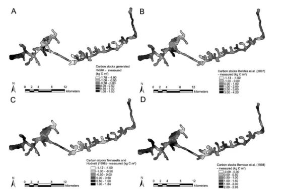
The spatial variability maps of the residuals as well as the statistics of the residuals are shown in Figures 5A, B, C and D and Table 7, respectively. The residual class-es shown in Figurclass-es 5A and C confirmed that the PTFs generated in this study and those developed by Tomasel-la and Hodnett (1998) presented the lowest residual and tend to underestimate even more the SOC stock, mainly when compared to the maps generated by Benites et al. (2007) and Bernoux et al. (1998). These results are in ac-cordance with the values of the MPE index previously discussed in item 3.2. We highlight the overestimation of SOC stock when applying the PTFs generated by Benites et al. (2007) and Bernoux et al. (1998). Using these PTFs, the overestimation of SOC stock could reach up to 4.20

and 2.95 kg cm−2_{, respectively (Figures 5B and D). The}

mean value of the SOC stock applying the PTF function generated in this study is practically the same of that in

the reference map (7.49 Mg C ha−1_{). On the other hand,}

applying the PTFs developed by Benites et al. (2007) and Bernoux et al. (1998), resulted in mean values of SOC

stock of 8.56 and 8.73 Mg C ha−1_{, respectively. When}

applying these PTFs, the mean residual value of SOC stock in relation to the reference map is 1.06 and 1.23

Mg C ha−1_{, a mean overestimation of 15 and 17 %,}

re-Figure 4 − Spatial variability maps of SOC stock using ordinary kriging. A) Map generated with the measured data of D_b; B) Map based on the

D_b estimated using the PTF generated in this work; C) Map based on the D_b estimated using the PTF generated by Benites et al. (2007); D)

Map based on the D_b estimated using the PTF generated by Tomasella and Hodnett (1998); E) Map based on the D_b estimated using the PTF generated by Bernoux et al. (1998). SOC = Soil Organic Carbon; PTFs = Pedotransfer functions.

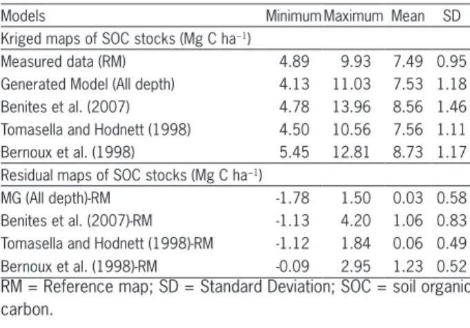
Table 7 − Statistics of the SOC stock maps and the residual caused by the application of different PTFs.

Models Minimum Maximum Mean SD

Kriged maps of SOC stocks (Mg C ha−1₎

Measured data (RM) 4.89 9.93 7.49 0.95

Generated Model (All depth) 4.13 11.03 7.53 1.18

Benites et al. (2007) 4.78 13.96 8.56 1.46

Tomasella and Hodnett (1998) 4.50 10.56 7.56 1.11

Bernoux et al. (1998) 5.45 12.81 8.73 1.17

Residual maps of SOC stocks (Mg C ha−1₎

MG (All depth)-RM -1.78 1.50 0.03 0.58

Benites et al. (2007)-RM -1.13 4.20 1.06 0.83

Tomasella and Hodnett (1998)-RM -1.12 1.84 0.06 0.49

Bernoux et al. (1998)-RM -0.09 2.95 1.23 0.52

RM = Reference map; SD = Standard Deviation; SOC = soil organic carbon.

spectively (Table 7). Considering the residuals found in this work, the error in the estimation of SOC stocks,

us-ing different PTFs to estimate D_b could be higher than

10 %, as previously reported by Bernoux et al. (1998). The results here presented can also give support to answer a significant and generic problem with the estimation of changes in terrestrial biospheric carbon, which is the smallest detectable change. The smallest difference in SOC stock that could be detected after 5 years under an herbaceous bioenergy crop was about 1

Mg C ha−1 _{in the southeastern United States (Garten and}

of SOC stock caused by applying the PTFs developed by Benites et al. (2007) and Bernoux et al. (1998) in the study site, it is possible to conclude that the simple

appli-cation of a PTF to estimate D_b could introduce an error

enough to offset the smallest detectable change of the SOC stock estimate.

Conclusions

A linear regression model was generated to

esti-mate D_b for soils of the Central Amazon region, Brazil.

The developed PTF used soil attributes easily found in soil survey reports such as SOC, pH in water, sum of

ba-sic cations, Al+3_{,and clay content as predictor of D}

b. The PTF generated should only be used in regions belonging to the Içá Geological Formation and covered with forest.

Compared to the three most used PTFs to estimate

D_b in Amazon soils (Bernoux et al., 1998; Tomasella and

Hodnett, 1998; Benites et al., 2007), our PTF outper-formed the other models, showing not only better ac-curacy, but also the lowest bias.

We also quantified the effect of using PTFs to

es-timate the D_b on spatial variability of SOC stock. The

results showed that the uncertainty caused by the

esti-mative of D_b using PTFs could be much higher than the

values reported in the literature. The PTFs of Benites et al. (2007) and Bernoux et al. (1998) caused an

overesti-mation of 1.06 and 1.23 Mg C ha−1 _{in the SOC stock,}

which represented 15 % and 17 %, respectively. This

means that the simple application of a PTF to estimate

D_b could introduce an error large enough to skew the

significant difference in soil carbon stock change.

Acknowledgements

The authors acknowledge Petrobras for the finan-cial support to perform this study (Contract Petrobras/ UFRRJ (Federal Rural University of Rio de Janeiro) / FAPUR (Foundation for Scientific and Technological

Re-search Support of UFRRJ), No _{0050.0036944.07.2). The}

authors thank the Rio de Janeiro State Foundation for Research Support (project number E-26/100.401/2013).

References

Adams, W.A. 1973. The effect of organic matter on the bulk and true densities of some uncultivated podzolic soils. Journal of Soil Science 24: 10-17.

Barros, H.S.; Fearnside, P.M. 2015. Pedo-transfer functions for estimating soil bulk density in Central Amazonia. Revista Brasileira de Ciência do Solo 39: 397-407.

Benites, V.M.; Machado, P.L.O.A.; Fidalgo, E.C.C.; Coelho, M.R.; Madari, B.E. 2007. Pedotransfer functions for estimating soil bulk density from existing soil survey reports in Brazil. Geoderma 139: 90-97.

Bernoux, M.; Arrouays, D.; Cerri, C.; Volkoff, B.; Jolivet, C. 1998. Bulk densities of Brazilian Amazon soils related to other soil properties. Soil Science Society of America Journal 62: 743-749.

Figure 5 − Spatial variability maps of the SOC stock residual. A) Residual based on the D_b estimated by the PTF generated in this work; B) Residual

based on the D_b estimated using the PTF generated by Benites et al. (2007); C) Residual based on the D_b estimated of the PTF generated using Tomasella and Hodnet (1998); D) Residual based on the D_b estimated using the PTF generated by Bernoux et al. (1998). SOC = Soil Organic

Bernoux, M.; Carvalho, M.C.S.; Volkoff, B.; Cerri C.C. 2002. Brazil’s soil carbon stocks. Soil Science Society of America Journal 66: 888-896.

Bouma J. 1989. Using soil survey data for quantitative land evaluation. Advances in Soil Science 9: 177-213.

Ceddia, M.B.; Villela A.L.O.; Pinheiro, E.F.M.; Wendroth, O. 2015. Spatial variability of soil carbon stock in the Urucu river basin, Central Amazon-Brazil. Science of the Total Environment 526: 58-69.

Deng, H.; Ye, M.; Schaap, M.G.; Khaleel, R. 2009. Quantification of uncertainty in pedotransfer function-based parameter estimation for unsaturated flow modeling. Water Resources Research 45: W04409. DOI:10.1029/2008WR007477.

De Vos, B.; Meirvenn, M.V.; Quatae, P.; Decker, J.; Muys, B. 2005. Predictive quality of pedotransfer functions for estimating bulk density of forest soils. Soil Science Society of America Journal 69: 500-510.

Empresa Brasileira de Pesquisa Agropecuária [EMBRAPA]. 1997. Manual of Methods of Soil Analysis = Manual de Métodos de Análises de Solo. 2ed. Embrapa-CNPS, Rio de Janeiro, RJ, Brazil (in Portuguese).

Empresa Brasileira de Pesquisa Agropecuária [EMBRAPA]. 1999. Brazilian System of Soil Classification = Sistema Brasileiro de Classificação de Solos. 2ed. Embrapa, Brasília, DF, Brazil (in Portuguese).

Garten, C.T.; Wullschleger, S.D. 1999. Soil carbon inventories under a bioenergy crop (Switchgrass): measurement limitations. Journal of Environmental Quality 28: 1359-1365.

Han, G.Z.; Zhang, G.L.; Gong, Z.T.; Wang, G.F. 2012. Pedotransfer functions for estimating soil bulk density in China. Soil Science 177: 158-164.

Harrison, A.F.; Bocock, K.L. 1981. Estimation of soil bulk-density from loss-on-ignition values. Journal of Applied Ecology 8: 919-927.

Heuscher, S.A.; Brandt, C.C.; Jardine, M.P. 2005. Using soil physical and chemical properties to estimate bulk density. Soil Science Society of America Journal 106: 52-62.

Howard, P.J.A.; Lovel, P.J.; Bradley, R.I.; Dry, F.T.; Howard, D.M. 1995. The carbon content of soil and its geographical distribution in Great Britain. Soil Use Management 11: 9-15.

Huck, S.W. 2012. Reading Statistics and Research. 6ed. Pearson, Boston, MA, EUA.

Leonaviciute, N. 2000. Predicting soil bulk and particle densities by pedotransfer functions from existing soil data in Lithuania. Geografijos Metraõtis 33: 317-330.

Manrique, L.A.; Jones, C.A. 1991. Bulk density of soils in relation to soil physical and chemical properties. Soil Science Society of America Journal 55: 476-481.

Moraes, J.L.; Cerri, C.C.; Melillo, J.M.; Kicklighter, D.; Neill, C.; Skole, D.L.; Steudler, P.A. 1995. Soil carbon stocks of the Brazilian Amazon basin. Soil Science Society of America Journal 59: 244-247.

RADAMBRASIL Project. 1978. SB.20 Purus: Geology, Geomorphology, Pedology, Vegetation and Potential Land Use = SB.20 Purus: Geologia, Geomorfologia, Pedologia, Vegetação e Uso Potencial da Terra. Ministério das Minas e Energia, Rio de Janeiro, RJ, Brazil. p. 566. (in Portuguese).

Sequeira, C.H.; Wills, S.A.; Seybold, C.A.; West, L.T. 2014. Predicting soil bulk density for incomplete databases. Geoderma 213: 64-73.

Tomasella, J.; Hodnett, M.G. 1998. Estimating soil water retention characteristics from limited data in Brazilian Amazonia. Soil Science 163: 190-202.

Vieira, S.R.; Hatfield, J.L.; Nielsen, D.R.; Biggar, J.M. 1983. Geostatistical theory and application to variability of some a agronomical properties. Hilgardia 51: 1-75.

Wackernagel, H. 2003. Multivariate Geostatistics: An Introduction with Applications. 3ed. Springer, Berlin, Germany.

Walkley, A.; Black, I.A. 1932. An examination of the Degtsjareff method for determining soil organic matter and proposed modification of the cromic acid titulation method. Soil Science 37: 29-38.