Spectrum and fine spectrum of the lower triangular matrix B r s t  , ,  over the sequence space cs

Original Article

Spectrum and fine spectrum of the lower triangular matrix



, ,



B r s t

over the sequence space

_cs

Rituparna Das

1*

_{and Binod Chandra Tripathy}

2

1 _{Department of Mathematics,}

Sikkim Manipal Institute of Technology, Majitar, Sikkim, 737136 India.

2 _{Department of Mathematics,}

Tripura University, Suryamaninagar, Agartala, Tripura, 799022 India.

Received: 16 April 2015; Accepted: 9 November: 2015

Abstract

Fine spectra of various matrix operators on different sequence spaces have been examined by several authors. Recently, some authors have determined the approximate point spectrum, the defect spectrum and the compression spectrum of various matrix operators on different sequence spaces. Here in this article we have determined the spectrum and fine spectrum of the lower triangular matrix B r s t



, ,



on the sequence space cs. In a further development, we have also determined the approximate point spectrum, the defect spectrum and the compression spectrum of the operator B r s t



, ,



on the sequence space cs. Keywords: spectrum of an operator, matrix mapping, sequence space

1. Introduction

By w, we denote the space of all real or complex valued sequences. Throughout the article c c bv bs, , , , , ₀  ₁ 

represent the spaces of all convergent, null, bounded varia-tion, bounded series, absolutely summable and bounded sequences respectively. Also bv₀ denotes the sequence space

0

bv c .

Fine spectra of various matrix operators on different sequence spaces have been examined by several authors. The spectrum and fine spectrum of the Zweier Matrix on the sequence space ₁ and bv was studied by Altay and Karaku (2005). Altay and Ba ar (2004, 2005) determined the fine spectrum of the difference operator  and the generalized difference operator B(r,s) on the sequence spaces c₀ and c. Furkan et al. (2006) have determined the fine spectrum of the generalized difference operator B(r,s) over the sequence

spaces 1 and bv. Altun (2011a, 2011b) determined the fine

spectrum of triangular Toeplitz operators and tridiagonal symmetric matrices over some sequence spaces. The fine spectra of the Cesàro operator C₁ over the sequence space





, 1

p

bv   p was determined by Akhmedov and Ba ar (2008). Okutoyi (1990) determined the spectrum of the Cesàro operator C₁ on the sequence space bv₀. Fine spectra of operator B r s t



, ,



over the sequence spaces 1 and bv and

generalized difference operator B(r,s) over the sequence spaces p and bvp, 1



  p



, were studied by Bilgiç and

Furkan (2007, 2008). Fine spectrum of the generalized differ-ence operator _v on the sequence space 1 was investigated

by Srivastava and Kumar (2010). Panigrahi and Srivastava (2011, 2012) studied the spectrum and fine spectrum of the second order difference operator 2

uv

 on the sequence space

c₀ and generalized second order forward difference operator

2 uvw

 on the sequence space 1. Fine spectra of upper

triangu-lar double-band matrices U(r,s) over the sequence spaces c₀

and c was studied by Karakaya and Altun (2010). Karaisa and Ba ar (2013) have determined the spectrum and fine spectrum of the upper triangular matrix A(r,s,t) over the sequence space



0



p  p 



. In a further development, they have also * Corresponding author.

Email address: rituparnadas_ghy@rediffmail.com; ri2p.das@gmail.com

determined the approximate point spectrum, defect spectrum and compression spectrum of the operator A(r,s,t) on the sequence space

_

_p



0 p 



.The approximate point spectrum, defect spectrum and compression spectrum of the operator B(r,s) on the sequence spaces c c0, ,p and bvp,



1  p



were studied by Ba ar, Durna and Yildirim (2011). The notion of matrix transformations over sequence space has been studied from various aspects. Besides the above listed workers, the spectrum and fine spectrum for various matrix operators has been investigated by Tripathy and Das (2014, 2015), Tripathy and Pal (2013a, 2013b, 2014), Tripathy and Saikia (2013) and many others in recent years.

In this paper, we will determine the spectrum and fine spectrum of the lower triangular matrix B(r,s,t) on the sequence space cs. Also, we will determine the approximate point spectrum, the defect spectrum and the compression spectrum of the operator B(r,s,t) on the sequence space cs.

Clearly,



 



0

: lim n

n i

n _i

cs x x w x exists

 _

  



is a Banach

space with respect to the norm

0

sup n _i

cs

n i

x x







.

2. Preliminaries and Background

Let X and Y be Banach spaces and T X: Y be a bounded linear operator. By R T

 

, we denote the range of

T, i.e.

  

: ,



R T  y Y y Tx x X   .

By B(X), we denote the set of all bounded linear operators on X into itself. If T B X

 

, then the adjoint T* _{of T is a}

bounded linear operator on the dual X* _{of X defined by}

 

_{T f}*

 

_{x  f Tx}

 

_{, for all} *

f X and x X .

Let X 

 

 be a complex normed linear space and

 

:

T D T X _{be a linear operator with domain D T}

 

 _X. With T, we associate the operator

T  T I,

where  is a complex number and I is the identity operator on

D(T). If T_ has an inverse which is linear, we denote it by _T 1



_,

that is





1 1

T T I

  _{  ,}

and call it the resolvent operator of T.

Let X 

 

 be a complex normed linear space and

 

:

T D T X be a linear operator with domain D T

 

 X. A regular value  of T is a complex number such that

(R1) _T 1



 _exists,

(R2) _T 1



 _{is bounded,}

(R3) _T 1



 _{is defined on a set which is dense in X i.e.}

 

R T_  X .

The resolvent set of T, denoted by 



T X,



, is the set of all regular values  of T. Its complement 



T X,









\ ,

C  T X in the complex plane C is called the spectrum

of T. Furthermore, the spectrum 



T X,



is partitioned into three disjoint sets as follows:

The point (discrete) spectrum p



T X,



is the set

such that _T 1

 does not exist. Any such   p



T X,



is

called an eigenvalue of T.

The continuous spectrum _c



T X,



is the set such that _T 1

 exists and satisfies (R3), but not (R2), that is, T1 is

unbounded.

The residual spectrum _r



T X,



is the set such that

1

T exists (and may be bounded or not), but does not satisfy

(R3), that is, the domain of _T 1

 is not dense in X.

If X is a Banach space and T B X

 

, then there are three possibilities for R(T) and _T1_:

(I) R T

 

 X,

(II) R T

 

R T

 

 X, (III) R T

 

 X , and

(1) _T1_{exists and is continuous,}

(2) _T1_{exists but is discontinuous,}

(3) _T1_{does not exist.}

(One may refer to Goldberg (1985))

Applying Goldberg’s classification to T, we have

three possibilities for T and T1

_;

(I) T is surjective,

(II) R T

 

 R T

 

 X,

(III) R T

 

  X,

and

(1) Tis injective and T1

 _{is continuous,}

(2) Tis injective but T1

 _{is discontinuous,}

(3) Tis not injective.

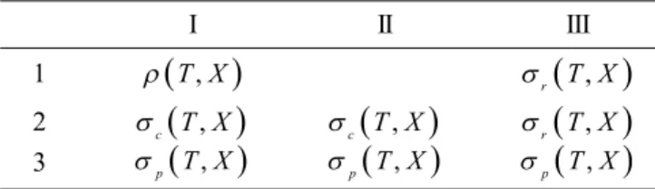
If these possibilities are combined in all possible ways, nine different states are created which may be shown as in Table 1.

These are labeled by: I I I II II II III III₁, ₂, ,_{3 1}, ₂, ₃, ₁, ₂

and . If  is a complex number such that TI₁ or TII1,

then  is in the resolvent set 



T X,



of T. The further classi-fication gives rise to the fine spectrum of T. If an operator is in state II₂ for example, then R T

 

R T

 

 X and 1

T

exists but is discontinuous and we write II2



T X,



.

Again, following Appell et al. (2004), we define the three more subdivisions of the spectrum called as the

approximate point spectrum, defect spectrum and compres-sion spectrum.

Table 1. Subdivisions of spectrum of a linear operator

I II III

1 



T X,



_r



T X,



2 c



T X,



c



T X,



r



T X,



Given a bounded linear operator T in a Banach space

X, we call a sequence (x_k) in X as a Weyl sequence for T if 1

k

x  and Tx_k 0 as k .

The approximate point spectrum of T, denoted by



,



ap T X

 , is defined as the set



,

 

:



ap T X C there exists a Weyl sequence for T I

   

(2.1) The defect spectrum of T, denoted by _



T X,



, is defined as the set



T X,

 

C T: I is not surjective





    (2.2)

The two subspectra given by (2.1) and (2.2) form a (not necessarily disjoint) subdivisions



T X,



ap



T X,







T X,



  _ (2.3)

of the spectrum. There is another subspectrum, _co



T X,











C R T: I  X



which is often called the compression spectrum of T. The compression spectrum gives rise to another (not necessarily disjoint) decomposition



T X,



ap



T X,



co



T X,



  _ (2.4)

Clearly, _p



T X,



_ap



T X,



and co



T X,







T X,



.

Moreover, it is easy to verify that



,





,



\



,



r T X co T X p T X

   and



,





,



\





,





,





c T X T X p T X co T X

   

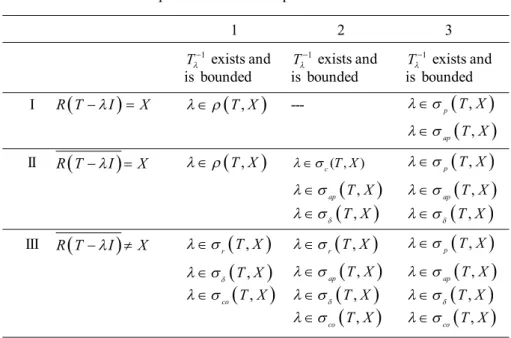
By the definitions given above, we can illustrate the subdivisions spectrum in Table 2.

Proposition 2.1. [Appell et al. (2004), Proposition 1.3, p.28]: Spectra and subspectra of an operator T B X

 

and its adjoint _T*_{B X}

 

* _{are related by the following relations:}

(a)



* *







, ,

T X T X

  .

(b)



* *







, ,

c T X ap T X

  .

(c)



* *







, ,

ap T X  T X

  .

(d)



* *







, _ap ,

T X T X



  .

(e)



* *







, ,

p T X co T X

  .

(f)



* *







, ,

co T X p T X

  .

(g)











* *



, _ap , _p ,

T X T X T X

  







* *



, ,

p T X ap T X

 

  .

The relations (c)–(f) show that the approximate point spectrum is in a certain sense dual to defect spectrum, and the point spectrum dual to the compression spectrum.

The equality (g) implies, in particular, that 



T X,







,



ap T X

 if X is a Hilbert space and T is normal.

Roughly speaking, this shows that normal (in particu-lar, self-adjoint) operators on Hilbert spaces are most similar to matrices in finite dimensional spaces (Appell et al., 2004).

Let  and  be two sequence spaces and A

 

a_nk be an infinite matrix of real or complex numbers a_nk, where





0

, 0,1, 2,...

n k N  . Then, we say that A defines a matrix

mapping from  into , and we denote it by A: , if for every sequence x

 

x_k , the sequence Ax



 

Ax _n



, the A-transform of x, is in , where

 

0

0

,

nk k n

k

Ax a x n N









 , (2.5)

Table 2. Subdivisions of spectrum of a linear operator

1 2 3

1

T exists and T1 exists and T1 exists and

is bounded is bounded is bounded I R T



I



 X  



T X,



---   p



T X,





,



ap T X

 

II R T



I



 X  



T X,



  _c( , )T X   p



T X,





,



ap T X

    _ap



T X,





T X,





    



T X,



III R T



I



 X   _r



T X,



  _r



T X,



  p



T X,





T X,





    ap



T X,



  ap



T X,





,



co T X

    _



T X,



  _



T X,





,



co T X

By



 :



, we denote the class of all matrices such that A:. Thus, A



 :



if and only if the series on the right hand side of (2.5) converges for each n N 0 and

every x, and we have



 



0

n n N

Ax Ax _  for all x. The lower triangular matrix B(r,s,t) is an infinite matrix of the form

 

0 0 0 0 0

, , 0

0

r s r

B r s t t s r

t s r



 

 

 

 

 

 

 

 

   

    

.

We assume here and hereafter that s and t are complex para-meters which do not simultaneously vanish.

The following results will be used in order to establish the results of this article.

Lemma 2.2 [Wilansky (1984), Example 6B, Page 130].The matrix A

 

a_nk gives rise to a bounded linear operator

 

T B cs from cs to itself if and only if

(i) , 1

1

sup m _{nk n k}

m k n

a a 



  

 

(ii) nk n

a



is convergent for each k.

Lemma 2.3 [ Golberg (1985), Page 59] T has a dense range if and only if T* _{is one to one.}

Lemma 2.4 [ Golberg (1985), Page 60] T has a bounded inverse if and only if T* _{is onto.}

3. Spectrum and fine spectrum of the operator B(r,s,t) on the sequence space cs

In this section, the fine spectrum of the operator

B(r,s,t) on the sequence space has been examined.

Before giving the main theorem we should give the following remark. In this work, here and in follows, if z is a complex number then by z we always mean the square root of with non-negative real part. If Re

 

z 0 then z rep-resents square root of z with Im

 

z 0. The same results are obtained if z represents the square root.

Theorem 3.1 B r s t cs



, , :



cs is a bounded linear operator and B r s t



, ,



_{( :cs cs)} r  s t .

Proof: From Lemma 2.2, it is easy to show that B r s t



, , :



cscs is a bounded linear operator.. Now,









1 2

0 0 0

1 2

0 0 0

, , ( ) n _i n _i n _i

i i i

n n n

i i i

i i i

cs

B r s t x rx sx tx

r x s x t x

r s t x

 

  

 

  

  

  

  













and hence, B r s t



, ,



( :cs cs) r  s  t .

Theorem 3.2If s is a complex number such that 2

s  s, then 



B r s t cs



, , ,





S where









2

2

: 1

4

r

S C

s s t r

 





  

   

 

 

 

 

 .

Proof: We shall prove this theorem by showing that









1

, ,

B r s t I 

 exists and is in



cs cs:



for S, and then show that the operator B r s t , ,









I is not invertible for S.

Without loss of any generality we assume that _s2 _

s

 . Let S. Clearly r and so B r s t



, ,



I is a tri-angle, therefore









1

, ,

B r s t I 

 exists. Let y 

 

y_n cs. Solving



B r s t



, ,



I x y



 for x in terms of y we get

















0 0

0 1

1 2

2

0

21 1

2 2 3

y x

r

sy y

x

r r

s t r y

y sy

x

r r r



 



  

 



 

 

   

  

  

 _{ }



Let us denote













2

1 2 2 3 3

1 _, s _, s t r

a a a

r r r



  

 



  

  

etc.

Then, we have

0 1 0 1 1 1 2 0 2 1 2 2 1 3 0

1 2 1 3 2 1 0 1

0

.

n

n n n n n n k k

k

x a y x a y a y x a y a y a y

x a y a y a y  a y a  y





 

  

     















 

1

2 1

1 3 2 1

4 3 2 1

5 4 3 2 1

0 0 0 0 0 0 0 0 0 , ,

0

nk a

a a

a a a

B r s t I a

a a a a

a a a a a

 

  

 

 

 

 

 

 

 

 

 

    

     

Also, from



B r s t



, ,



I x y



 , we have y_n tx_n₂sx_n₁



r 



xn

  .

Using the recurrence relation ₁

0

n

n n k k

k

x a   y







we get





2 1

1 1

0 0 0

n n n

n n k k n k k n k k

k k k

y t  a_{ } y s a y _ r  a_{ } y

  









 



y ta0



n1san 



r 



an1



y ta1



n2san1



r



an



  y a rn 1







.

This gives





















1 1

2 1

1

0 0

1

n n n

n n n

ta sa r a

ta sa r a

a r

 



 

 

   

   

 



This sequence can be obtained recursively by putting









1 2 2 2 1

1

, , n n n 0, 3

s

a a ta sa r a n

r  r    



      

  .

The characteristic equation of the recurrence relation is



_{r }



2_{s t 0.}

Then we have two cases:

Case 1: Let _{D s} 2_{4t r}



_



_0.

Then the roots of the characteristic equation are









1 and 2 .

2 2

s D s D

r r

 

 

   

 

 

It is easy to show that 1 2 _{, 1}

n n

n

a n

D

 

  .

Since S, so ₁ 1 and therefore we have





2

2

1 D r

s s





 

 .

Since, 1 z  1 z for all z C _{, so}





2

2

1 D r

s s





 



and hence ₂ 1.

It is easy to show that for all m,



, 1



1 2

1 0 0 0

1

m m m m

n n

nk n k n

k n n n n

a a a

D  



   

  



_





_





 







(3.1)

and hence, _{, 1}

1

sup m ( nk n k )

m _{k n}

a a  

  

 

, as 1 1 and 2 1.

Since 1 1 and 2 1, so for all k, the series

1 2 3

nk n

a a a a 



 (3.2)

is absolutely convergent and hence convergent. So, by Lemma 2.2,









1

, ,

B r s t I 

 is in



cs cs:



. This shows that 



B r s t cs



, , ,





S.

Next let S. If r then B r s t



, ,



I is re-presented by the matrix





0 0 0 0 0 0 0

0, , 0 0

0 0

s B s t t s

t s



 

 

 

 

 

 

 

 

        

.

Since B r s t



, ,



rI B (0, , )s t does not have a dense range, it is not invertible.

So we may assume that  r. Since 2 ₄





₀

D s  t r 

therefore we must have ₁  ₂ , from which we have

lim _n 0

na  and so for all k, the series

1 2 3

nk n

a a a a 





is divergent. Therefore









1

, ,

B r s t I 

 is not in



cs cs:



and hence S 



B r s t cs



, , ,





.

Case 2: Let 2





4 0

D s  t r  . Then for all n1, we get





2 2

n

n

n s

a

s r 

 

 

















_

_

Since S, so





1

2

s r 

 

 .

Then for all m,



, 1



1 0 0

m m

nk n k n n

k n n n

a a  a  a

  

  

 





and hence, _{, 1}

1

sup m ( _{nk n k} )

m k n

a a 



  

 

, as





1

2

s r 

 

Since





1

2

s r 

 

 , so for all k, the series

1 2 3

nk n

a a a a 





is absolutely convergent and hence convergent. So, by Lemma 2.2,









1

, ,

B r s t I 

 is in



cs cs:



. This shows that 



B r s t cs



, , ,





S.

Next let S. Then we have





1

2

s r 

 

 from

which we get lim n 0

na  and so for all k, the series

1 2 3

nk n

a a a a 





is divergent. Therefore









1

, ,

B r s t I 

 is not in



cs cs:



and hence S 



B r s t cs



, , ,





.

Thus in each case we get 



B r s t cs



, , ,





S. This completes the proof.

Remark: If _s2 _{s, then we obtain the same sequence and}

















2 2

, , , : 1

4

r B r s t cs C

s s t r



 

 

  

  





















.

Theorem 3.3The point spectrum of the operator B r s t( , , )

over is given byp



B r s t cs



, , ,





 .

Proof: Let  be an eigenvalue of the operator ( , , )B r s t . Then there exists x  (0, 0, 0,...) in cs such that B r s t x



, ,



x

, ,

B r s t xx.

Then, we have

0 0

0 1 1

0 1 2 2

1 2 3 3

2 1 , 2

n n n n

rx x sx rx x tx sx rx x tx sx rx x

tx sx rx x n

 

 



 



 

  

  

   



If x_k is the first non-zero entry of the sequence ( )xn , then

r

  . Then from the relation tx_k1sx_k rx_k1 x_k1, we have x_k 0, a contradiction.

Hence, _p



B r s t cs



, , ,





 . This completes the proof. If T cs: cs is a bounded linear operator represented by a matrix A, then it is known that the adjoint operator

* * *

:

T cs cs is defined by the transpose _At _{of the matrix A.}

It should be noted that the dual space _cs* _{of cs is}

isometri-cally isomorphic to the Banach space bv of all bounded varia-tion sequences normed by 1

0

lim

n n n

bv _n

n

x  x x _ x







  .

Theorem 3.4The point spectrum of the operator





* , ,

B r s t

over *

cs is given by







* *



1

, , ,

p B r s t cs bv S

   , where









1 ₂

2

: 1

4

r

S C

s s t r

 





  

   

 

 

 

 

 

.

Proof: Let  be an eigenvalue of the operator





* , ,

B r s t . Then there exists x 



0, 0, 0,_



in bv such that





*

, ,

B r s t

x = ax. Then, we have





0 1 2 0

1 2 3 1

2 3 4 2

1 2

, ,

, 0.

t

n n n n

B r s t x x rx sx tx x

rx sx tx x rx sx tx x

rx sx tx x n

 

 



 



   

  

  

   



It is clear that if  = r then we may choose x₀ 0 and x =



0, 0,0,0,...



x x is an eigenvector corresponding to  = r. Assume that  r.

Then, we have

















2 1 0

2

3 2 1 2 0

1

1 0

1 1 , 2 .

n n

n n

n n n

s r

x x x

t t

s t r s r

x x x

t t

a r a r

x x x n

t t



 

  

 

 

 

  

 

 

  



If S1, then we may choose









0 1 ₂

2 1,

4

r

x x

s s t r

 



 

   

.

We now show that

 

₁ n, 2

n

x  x n .

Since ₁ and ₂ are roots of the characteristic equation





2

0

r  s t , therefore

1 2 , 1 2

t D

r r

   

 

  

where









1 , 2

2 2

s D s D

r r

 

 

   

 

  and





2 ₄

D s  t r

0

 .

Clearly ₁

1 1

x



 . Then we have























 

1 1 0 1 1 1

1 0 1

1 1 1 1

1 2 1 2 1

1 1 2

1 1 2

2

1 1

1 2 1 2 1

1 1 , 2 1 1 1 1 n n n n

n n n

n

n n

n n n n

n

n

n n

n

n

a r a r

x x x n

t t

r

r a x a x

t r D x                                                       





































If 2





4 0

D s  t r  then also we may get the same result.

Now, 1

1 1 1 1

0 0 0 0 0

n n

n n n n

n n n n n

x x x x x x

    



 

    

      











as

1 1

x  . Therefore x bv .

Hence







* *



1 p , , ,

S  B r s t cs bv .

Next assume that S₁. Then









2 2 1 4 r

s s t r

 





    and

so 1 1. We must show that









* *

, , ,

p B r s t cs bv

   .

Using





1





1 0

1 1 , 2

n n

n n

n n n

a r a r

x x x n

t t

 _ 

 

 

   _{, we get}

1 0 1 1 1 0 1 1 n

n n n

n

n n

n

a

x x

x r a a

a

x t a _{x x}

a           













_

_











_



_





.

We now consider three cases: Case (i): ₂  ₁ 1

In this case _{D s} 2_{4t r}



_



_{0 and}

1

1 2

1

1 1

1

1 1 2

1

1 1 2 ₂

1

1

1

lim lim lim lim

1 n n n n n n n n n

n n n n

n n n

a a a a         _                      _{ }    _{ }       _{ }    _{ }     

Now, if  x₀ _{1 1}x 0, then we get 0 1

n n

x x



 . Since ₁ 1,

therefore

 

xn c and so

 

xn bv. Otherwise

1

1

1 2 2

1 1

lim n 1

n n

x

x    



    .

Case (ii): ₂  ₁ 1.

In this case 2 ₄





₀

D s  t r  and a_n =





2 2 n n s a

s r 

            _{ }, 1

n . Then





1 1 2 lim 2 n n n a s

a r   

       and so 1 1

1 2 2

1 1

lim n 1

n n

x

x    



    .

Case (iii): ₂  ₁ 1

In this case 2





4 0

D s  t r  and we have 1 2

s t

  _.

Assume that







* *



, , ,

p B r s t cs bv

   . This implies that x bv and x.

Again from





1





1 0

1 1 , 2

n n

n n

n n n

a r a r

x x x n

t t

 _ 

 

 

   we get





1 0 1 1 2 2 n n s s

x n x nx

t t



 





_

 

_

_

 



_



_





_



 







Now, x bv and so x c . Therefore we must have x0 x1 

= 0. Which implies x, a contradiction. So   p







* *



, , ,

B r s t cs bv .

In case (i) and case (ii) above, we have

 

xn c

and so

 

x_n bv. In case (iii) by assuming   p







_{B r s t, ,} *_,cs* _bv



we get a contradiction. This completes the proof.

Theorem 3.5The residual spectrum of the operator B r s t



, ,



over cs is given by







, , ,



1

r B r s t cs S

Proof: Since,





_{, , ,}









_{, ,}



*_, *



_\ r B r s t cs p B r s t cs

 







, , ,



p B r s t cs

 , so we get the required result by using Theorem 3.3 and Theorem 3.4 .

Theorem 3.6 The continuous spectrum of the operator



, ,



B r s t over are given by _c



B r s t cs



, , ,





S₂ , where









2

2

2

: 1

4

r

S C

s s t r

 





  

   





















.

Proof: Since, 



B r s t cs



, , ,





is the disjoint union of







, , ,



p B r s t cs

 , r



B r s t cs



, , ,





and c



B r s t cs



, , ,





,

therefore, by Theorem 3.3, Theorem 3.4 and Theorem 3.5, we

get

















2

2

, , , : 1

4

c

r

B r s t cs C

s s t r



 





  

   

 

 

 

 

 .

Theorem 3.7 If  r, then III1



B r s t cs



, , ,





if

t  s and III2



B r s t cs



, , ,





if t  s .

Proof: If  r, the range of B r s t



, ,



is not dense. So, from Table 2 and Theorem 3.5, we have   r



B r s t cs



, , ,





.

From Table 2, we get _r



B r s t cs



, , ,























1 , , , 2 , , ,

III B r s t cs III B r s t cs .

Therefore, III1



B r s t cs



, , ,





or III2



B r s t cs



, , ,





.

Also for  r, B r s t



, ,



I B



0, ,s t



. A left inverse of B



0, ,s t



is









 

 

 

1 2

2

3 2

1

0 0 0

1

0 0

0, ,

1 0

s t

s s

B s t

t t

s

s s



 

 















































    

In other words









1

 

0, , _nk

B s t  b

 , where

 

1

2 , 1 2

0, 1 2

n k

n k

nk

t

if k n

b _s

if k or k n

   



   

  

   

Now for each m, we get



, 1



2 23 1 1

1 m

m

nk n k m

k n

t t t

b b

s s s s

 



     

 

 _{and so}



, 1



1

sup m nk n k

m k n

b b 





 

exists if and only if t  s .

Also for each k,

 

2

2 3

1

nk n

t t b

s s s

 

   



 is convergent if

and only if t  s .

Therefore, the matrix









1

0, ,

B s t 

is in



cs cs:



if t  s

and not in



cs cs:



if t  s . This completes the theorem.

Theorem 3.8 If  r and   _r



B r s t cs



, , ,





, then









2 , , ,

III B r s t cs

  .

Proof: Since,   _r



B r s t cs



, , ,





, therefore, from Table 2, we have III1



B r s t cs



, , ,





or III2



B r s t cs



, , ,





.

Now,   r



B r s t cs



, , ,





implies that

   

2

2

1 4

r

s s t r

 



    

and so ₁ 1

Therefore, the series (3.1) in Theorem 3.2 is not convergent and hence, the operator B r s t



, ,



has no bounded inverse. Therefore, III2



B r s t cs



, , ,





.

Theorem 3.9 The approximate point spectrum of the operator B r s t



, ,



over is given by _ap



B r s t cs



, , ,







 

\ ,

,

S r if t s S if t s

 







.

Proof: From Table 2, we have ap



B r s t cs



, , ,













B r s t cs III, , ,



\ 1



B r s t cs



, , ,





  .

Using Theorem 3.2 and Theorem 3.7, we get the required result.

Theorem 3.10 The compression spectrum of the operator



, ,



B r s t over is given by







, , ,



1

co B r s t cs S

  .

Proof: By proposition 2.1 (e), we get





_{, ,}



*_, *



p B r s t cs

 







, , ,



co B r s t cs

 .

Using Theorem 3.4, we get the required result.

Theorem 3.11The defect spectrum of the operator B r s t



, ,



over is given by







B r s t cs, , ,



S



Proof: From Table 2, we have 



B r s t cs



, , ,













B r s t cs I, , ,



\ 3



B r s t cs



, , ,





  . Also, p



B r s t cs



, , ,































3 , , , 3 , , , 3 , , ,

I B r s t cs II B r s t cs III B r s t cs.

By Theorem 3.3, we have p



B r s t cs



, , ,





  and so









3 , , ,

I B r s t cs  . Hence 



B r s t cs



, , ,





S.

COROLLARY 3.13The following statements hold:

(i)





_{, ,}



*_, *



ap B r s t cs bv S

   .

(ii)





_{, ,}



*_, *



\

 

, ,

S r if t s B r s t cs bv

S if t s



   









.

Proof: Using Proposition 2.1 (c) and (d), we get







_{, ,} *_, *







_{, , ,}





ap B r s t cs bv  B r s t cs

   and







_{, ,} *_, *







_{, , ,}





ap

B r s t cs bv B r s t cs



   .

Using Theorem 3.9 and Theorem 3.11, we get the required results.

References

Akhmedov, A.M. and Ba ar, F. 2008. The fine spectra of the Cesàro operator C₁ over the sequence space





, 1 p

bv  p  . Mathematics Journal of Okayama University. 50, 135-147.

Akhmedov, A.M. and El-Shabrawy, S. R. 2011. On the fine spectrum of the operator a b, over the sequence space

c, Computers and Mathematics with Applications. 61(10), 2994-3002.

Altay, B. and Ba ar, F. 2004. On the fine spectrum of the dif-ference operatoron c₀and c, Information Sciences. 168, 217-224.

Altay, B. and Ba ar, F. 2005. On the fine spectrum of the gener--alized difference operator B r s

 

, over the sequence spaces c₀and c, International Journal of Mathematics and Mathematical Sciences. 2005(18), 3005-3013. Altay, B. and Karaku , M. 2005. On the Spectrum and the fine

spectrum of the Zweier matrix as an operator on some sequence spaces, Thai Journal of Mathematics. 3(2), 153-162

Altun, M. 2011. On the fine spectra of triangular Toeplitz operators, Applied Mathematics and Computations. 217, 8044-8051.

Altun, M. 2011. Fine spectra of tridiagonal symmetric matrices, International Journal of Mathematics and Mathematical Sciences. Article ID 161209.

Appell, J., Pascale, E., and Vignoli, A. 2004. Nonlinear Spectral Theory, Walter de Gruyter, Berlin, New York, U.S.A. Ba ar, F., Durna, N., and Yildirim, M. 2011. Subdivisions of

the spectra for generalized difference operator over certain sequence spaces, Thai Journal of Mathema-tics. 9(2), 279-289.

Ba ar, F. 2012. Summability Theory and Its Applications, Bentham Science Publishers, e-books, Monographs, Istanbul.

Bilgiç, H. and Furkan, H. 2007. On the fine spectrum of operator B r s t



, ,



over the sequence spaces ₁ and, Mathematics and Computer Modelling. 45, 883-891. Bilgiç, H. and Furkan, H. 2008. On the fine spectrum of the

generalized difference operator B r s

 

, over the sequence spaces ₁ and bvp, (1 p ), Nonlinear

Analysis. 68, 499-506.

Bilgiç, H., Furkan, H., and Kayaduman, K. 2006. On the fine spectrum of the generalized difference operator

 

,

B r s over the sequence spaces ₁ and bv, Hokkaido Mathematical Journal. 35, 893-904.

Furkan, H., Bilgiç, H., and Altay, B. 2007. On the fine spectrum of operator B r s t



, ,



over c₀and c, Computers and Mathematics with Applications. 53, 989-998.

Furkan, H., Bilgiç, H., and Ba ar, F. 2010. On the fine spectrum of operator B r s t



, ,



over the sequence spaces p

and bvp, 1



 p 



, Computers and Mathematics

with Applications. 60, 2141-2152.

Golberg, S. 1985. Unbounded Linear Operators-Theory and Applications, Dover Publications, Inc, New York, U.S.A.

Gonzalez, M. 1985. The fine spectrum of the Cesàro operator

in _p



1_{  p}



_{, Archivum Mathematicum. 44,}

355-358,

Karaisa, A. and Ba ar, F. 2013. Fine spectrum of upper tri-angular triple-band matrices over the sequence space



1



p _{  p}

 , Abstract and Applied Analysis. Article ID 342682.

Karakaya, V. and Altun, M. 2010. Fine spectra of upper tri-angular double-band matrices, Journal of Computers and Applied Mathematics. 234, 1387-1394.

Kayaduman, K. and Furkan, H. 2006. The fine spectra of the difference operator  over the sequence spaces ₁ and bv, International Mathematics Forum,1(24), 1153-1160.

Kreysziag, E. 1989. Introductory Functional Analysis with Application,John Wiley and Sons, U.S.A.

Okutoyi, J.I. 1990. On the spectrum ofC₁ as an operator on

0

bv , Journal of the Australian Mathematical Society.. (Series A) 48, 79-86.

Panigrahi, B.L. and Srivastava, P.D. 2011. Spectrum and the fine spectrum of the generalised second order differ-ence operator 2

uv

 on sequence space c₀. Thai Journal of Mathematics, 9(1), 57-74.

Panigrahi, B.L. and Srivastava, P.D. 2012. Spectrum and fine spectrum of the generalized second order forward difference operator 2

uvw

 on the sequence space ₁, Demonstration Mathematica, XLV(3), 593- 609. Srivastava, P.D. and Kumar, S. 2010. Fine spectrum of the

generalized difference operator _v on the sequence space ₁. Thai Journal of Mathematics. 8(2), 221-233. Tripathy, B.C. and Das, R. 2014. Spectra of the Rhaly operator on the sequence space bv___0; Boletim da Sociedade

Paranaense de Matemática. 32(1), 263-275.

Tripathy, B.C. and Das, R. 2015. Spectrum and fine spectrum of the upper triangular matrix B r



, 0,s



over the sequence space, Applied Mathematics and Informa-tion Sciences. 9(4), 2139-2145. doi.org/10.12785/amis/ 090453

Tripathy, B.C. and Paul, A. 2013. Spectra of the operator

B(f, g) on the vector valued sequence space c₀(X). Boletim da Sociedade Paranaense de Matemática. 31(1), 105-111.

Tripathy, B.C. and Paul, A. 2013. The Spectrum of the operator D(r,0,0,s) over the sequence space c₀ and c. Kyungpook Mathematical Journal. 53(2), 247-256.

Tripathy, B.C. and Paul, A. 2014. The Spectrum of the Operator D(r,0,0,s) over the sequence spaces p and

bvp. Hacettepe Journal of Mathematics and Statistics.

43 (3), 425-434

Tripathy, B.C. and Saikia, P. 2013. On the spectrum of the Cesáro operator C₁ on bv___, Mathematica Slovaca.

63(3), 563-572.