Variability of the Lagrangian turbulent diffusion in the lower stratosphere

(1)

www.atmos-chem-phys.org/acp/5/1605/ SRef-ID: 1680-7324/acp/2005-5-1605 European Geosciences Union

Chemistry

and Physics

Variability of the Lagrangian turbulent diffusion in the lower

stratosphere

B. Legras1, I. Pisso1, G. Berthet2, and F. Lef`evre2

1_{Laboratoire de Météorologie Dynamique, UMR8539, Paris, France} 2_{Service d’Aéronomie, UMR7620, Paris, France}

Received: 28 October 2004 – Published in Atmos. Chem. Phys. Discuss.: 15 December 2004 Revised: 13 April 2005 – Accepted: 30 May 2005 – Published: 22 June 2005

Abstract.Ozone and nitrous oxide are measured at high

spa-tial and temporal resolution by instruments flying on the ER-2 NASA research aircraft. Comparing the airborne transects to reconstructions by ensemble of diffusive backward trajec-tories allows estimation of the average vertical Lagrangian turbulent diffusion experienced by the air parcels. The re-sulting estimates show large Lagrangian diffusion of the or-der of 0.1 m2s−1in the surf zone outside the polar vortex and smaller values of the order of 0.01 m2s−1 inside. Lo-cally, large variation of Lagrangian diffusion occurs over mesoscale distances. It is found that high temporal resolu-tion (3 h or less) is required for off-line transport calcularesolu-tions and that the reconstructions are sensitive to spurious motion in standard analysed winds.

1 Introduction

The distribution of chemical compounds in the atmosphere exhibits a large range of variability that is partly due to trans-port. This is particularly true in the lower stratosphere for species, like nitrous oxide N2O which have no sources or sinks in this region. Ozone is chemically reactive in the lower stratosphere but its lifetime exceeds several weeks except in the regions where chlorine is activated within the winter po-lar vortex; that is long enough for transport to be effective.

In the lower stratosphere, vertical motion is limited by stratification to be of the order of 1 K/day in potential temper-ature. Hence it takes about 3 weeks to travel over a vertical distance of 1 km and transport is mostly dominated by hor-izontal motion. With a vertical shear3_≈2 10−3s−1 and a horizontal strainγ_≈10−5s−1, a compact cloud of particles is first dispersed by vertical shear during a few hours until it reaches an equilibrium slope of3/γ_≈200 within about Correspondence to:B. Legras

([email protected])

one day after which dispersion is mainly due to the horizon-tal strain (Haynes and Anglade, 1997). Under the repeated action of strain and foldings due to the nonlinearity of the flow, tracers are stirred and form a number of sloping sheets which are observed as laminae in vertical soundings and air-craft transects. The core of intense jets, such as in the strato-spheric polar vortex, acts as a transport barrier and is often associated with strong tracer gradient.

The proof of this concept is provided by the ability to re-construct the small-scale distribution of tracers by advection methods using analysed winds (Waugh et al., 1994; Sutton et al., 1994; Mariotti et al., 1997). The basis of these methods is that layer-wise tracer advection in the stratosphere is dom-inated by the large scales of motion which are sufficiently well resolved by operational analysed winds provided by the major weather centers. This flow regime is known as the Batchelor regime in fluid dynamics (Haynes and Vanneste, 2004; Falkovich et al., 2001). Hence, the tracer structures at scales smaller than the analysed winds are to some extent predictable by integrating the advection equation backward in time (Methven and Hoskins, 1999). There is no contradic-tion here: the informacontradic-tion about unresolved tracer scales is fully contained in the time series of wind fields.

(2)

Konopka et al., 2004), our goal here is not to test a particu-lar parametrization but to provide an independent estimate of unresolved turbulent motion as an ordinary vertical diffusion

D.

The literature exhibits a variety of estimates of D rang-ing from 5 m2s−1to 0.001 m2s−1The largest values are ob-˙ tained from radar measurements assuming homogeneous tur-bulence and near critical Richardson number (Woodman and Rastogi, 1984; Fukao et al., 1994; Nastrom and Eaton, 1997). These values are contradicted by recent estimates from high resolution balloon data (Alisse et al., 2000) and by studies of large-scale advective stirring (Waugh et al., 1997; Balluch and Haynes, 1997) that provide values in the lower part of the range, of the order of 0.01 m2s−1or less.

Both estimates of Waugh et al. (1997) and Balluch and Haynes (1997) were based, like the present study, on the dominating layer-wise motion in the stratosphere to gener-ate tracer sheets. From the assumption that tracer structures are sloping sheets, Balluch and Haynes reduced locally the advection and the diffusion of a tracer to a one dimensional equation projected on an evolving gradient direction. They estimated an upper limit on vertical diffusivity by recon-structing several laminae selected from N2O airborne mea-surements, varying the diffusivity until the reconstruction best agrees with the observations. In this study, we go one step further by removing any assumption about tracer dis-tribution and using a powerful method to solve locally the advection-diffusion problem.

This new approach has been introduced in Legras et al. (2003) to study vertical diffusivity from the reconstruction of vertical ozone profiles. The conclusion of this study was to put an upper limit of 0.1 m2s−1 for the vertical diffusiv-ity in the lower stratosphere mid-latitude surf zone during winter. The possibility to test smaller values of the diffusiv-ity was, however, impaired by the limited vertical resolution of ozone soundings with standard chemical sondes that is of the order of 100 m if we stay on the optimistic side. Us-ing the slope factor 200, the equivalent horizontal resolution of ozone soundings does not exceed 20 km, while airborne tracer measurements are currently performed with resolution under 1 km for species like O3, CH4 or N2O that can be measured at high frequency of one to a few Hertz. Hence, airborne measurements resolve at least 20 times better the small-scale sloping structure than standard ozone soundings. The above motivates the present study which extends Legras et al. (2003) by analysing airborne transects collected by the instruments on board the NASA ER-2 during the SOLVE campaign in the Arctic in January–March 2000.

Section 2 presents the method used for the Lagrangian re-constructions based on the advective-diffusive equation. Sec-tion 3 describes the data and trajectory calculaSec-tions used in this study. Section 4 demonstrates that diffusive reconstruc-tions of a tracer are strikingly stable over a large range of reconstruction times. Section 5 defines the roughness crite-rion used to fit the vertical diffusion in this study. Section 6

discusses the reconstructions of the most significant SOLVE flights and the best fitting diffusivities. Section 7 discusses local structures. Section 8 discusses the relation between dif-fusivity and dispersion. Section 9 shows the spurious effects of under-resolving the temporal variations of the wind. Fi-nally, Sect. 10 offers further discussion, including a compar-ison with previous results of Balluch and Haynes (1997), and conclusions.

2 Diffusive reconstruction

The standard reconstruction method for the mixing ratio of a tracer at timet0within a given domainDconsists in finding the location, at an earlier timet0−τ, of the parcels fillingD at timet0, and to attribute a mixing ratio to each parcel ac-cording to the tracer mixing ratio at its initial location at time

t0−τ. The initial location is found by backward integration of the particle advection equationdx/dt₌u(x, t )where the windu(x, t )is interpolated in time and space from the anal-ysed winds provided by operational weather centers. The main interest of this calculation is that the reconstructed field at timet0 gives access to much smaller scales than the ini-tialisation field used at timet0−τ. In many previous stud-ies, the tracer was potential vorticity (PV) and it was ini-tialised according to the analysis from weather centers. The value of this approach has been demonstrated by compar-ing the reconstructed PV with observations of tracers, either in the stratosphere with aerosols and ozone (Waugh et al., 1994; Sutton et al., 1994; Mariotti et al., 1997; Orsolini et al., 2001) or in the troposphere with water vapour (Appenzeller et al., 1996). However, PV can hardly be measured by in situ instruments and cannot be assumed to correlate perfectly with any measurable tracer. Hence, recent efforts have been devoted to the direct reconstruction of observable chemical fields. The tracer distribution at timet0−τ is then provided, with a crude resolution, either by a chemical transport model (Legras et al., 2003) or by satellite observations (Orsolini et al., 2001).

The standard reconstruction method is purely advective and fully deterministic. It fails to take into account any diffu-sive process and generates a number of small-scale structures that increases exponentially with the reconstruction timeτ. It is usually considered that, according to the resolution of initial fields, reconstructions should be performed over dura-tions of 10 to 20 days in the lower stratosphere (Methven and Hoskins, 1999; Waugh and Plumb, 1994) beyond which the number of spurious structures pervades the results.

In our approach, as sketched in Fig. 1, diffusion is taken into account by splitting the parcel at timet0intoN particles which are all advected backward in time by the equation

δx=u(x, t )δt₊kδη(t ) , (1)

(3)

Fig. 1.Sketch of the trajectories of the transported and diffused par-ticles meeting in pointMat timet0after travelling from their initial locations(A, B, C, D)at timet0−τ. The mixing ratio inMandt0 is reconstructed from averaging the mixing ratios in(A, B, C, D) andt0−τ.

white noise process is without memory (i.e. it isδ-correlated in time), and with a zero mean. In the limitδt_→0 and after statistical average over a large number of particles, this is equivalent to adding a diffusionDto transport with

D₌1

2 < w 2_{> δt .}

(2)

In order to ensure that vertical velocities are bounded, we use a white noise based on a random variabler that is uni-formly distributed over the interval [−√3,√3] with zero mean and unit variance. Applying Eq. (2), the random pro-cess is thenδη₌r√2Dδt with a new drawing ofr at each time step and for each particle. Actually, we use a time-step of 18 s for the random term which is fifty times smaller than the time-step for advection in order to enhance statistical convergence.

The reconstructed mixing ratio of the parcel is the aver-age of the mixing ratios of theN particles initialised at time

t0−τ.

The method just described is directly related to the solu-tion of the advective-diffusive equasolu-tion for the mixing ratio

χof a passive tracer

χ (x, t )₌ Z

ρ(y, s)G(x, t_;y, s)χ (y, s)d3y, (3)

where G(x, t_;y, s) is the Green function describing the probability of a particle that was iny at time s to be inx at timet, andρ is air density. The Green functions satisfies

the two equations (Morse and Feschbach, 1953)

∂G

∂t +u(x, t )· ∇xG− D

ρ(x, t )∇xρ(x, t )∇xG

= 1

ρ(y, s)δ(t−s)δ(y−x) ,

(4)

∂G

∂s +u(y, s)· ∇yG+ D

ρ(y, t )∇yρ(y, t )∇yG

= 1

ρ(x, t )δ(t−s)δ(y−x) .

(5)

Here,the derivatives are taken with respect to the final coor-dinatesxandt for the first equation and with respect to the initial coordinatesyandsfor the second one. The statistical average of mixing ratio over random backward trajectories is equivalent to solving Eq. (5) up to neglecting the variations of

ρover turbulent diffusive scales. The negative sign in front of the diffusive term on the r.h.s. of Eq. (5) means that this equation is well-posed for backward integration in time. For a more detailed discussion, see Holzer and Hall (2000) and Issartel and Baverel (2003).

Notice that the random process entering the advection equation has been described here assuming that time-stepping is performed using a simple Euler scheme. More sophisticated numerical schemes require adequate transfor-mations.

3 Data and trajectory processing

(4)

9.6 9.7 9.8 9.9 10 10.1 10.2 0

1 2 3

∆

z

* (km)

(a)

Universal Time (hour)

N2

O (ppbv)

(b)

9.6 9.7 9.8 9.9 10 10.1 10.2 80

100 120 140 160 180 200

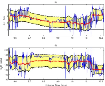
Fig. 2. (a): Vertical displacement 1z∗ of the particles with re-spect to their launch on the flight track, where z∗₌H0ln(p0/p) (p0=1000 hPa,H0=5850 m). In red: average displacement for the diffusive motion withD₌0.01 m2s−1. The yellow region spans one standard deviation from the average. In blue: displacement for a single deterministic particle with no diffusion. Results are shown for backward integration overτ₌38 days and one portion of the 27 January 2000 flight.(b): Same as (a) but for the reconstructed N₂O mixing ratio.

Reverse integrations of particles trajectories initialised along each transect have been performed with TRACZILLA, a modified version of the trajectory code FLEXPART (Stohl et al., 2002) which uses ECMWF (European Center for Medium range Weather Forecast) winds at 1◦horizontal res-olution and on 60 hybrid levels with 3-h resres-olution obtained by combining analysis available every 6 h with first guesses at intermediate times. The modifications from FLEXPART advection scheme consists mainly in discarding the interme-diate terrain following coordinate system and in performing a direct vertical interpolation of winds, linear in log-pressure, from hybrid levels. The vertical velocities used in this study are computed by the FLEXPART preprocessor using a mass conserving scheme in the hybrid ECMWF coordinates. A small correction due to a missing term in FLEXPART has been introduced but has virtually no impact. The model uses a fixed time step ofδt₌900 s. Halving it has no impact on our results. Unless stated differently, the reconstruction are performed by releasingN₌1000 particles every 4 s along the flight track that is about with the same frequency than the N2O measurements. We use the GPS ER-2 data and the on-board pressure sensor to locate the launching point, respec-tively horizontally and vertically. By launching the particles exactly on the flight track and also by performing a partial first time step to the nearest discretized time of the model, we take into account the short-time fluctuations in flight al-titude with which tracer fluctuations are correlated (Sparling and Bacmeister, 2001).

Assignment of N2O and O3was performed att0−τ loca-tion from three-dimensional fields produced by REPROBUS (REactive Processes Ruling the Ozone BUdget in the Strato-sphere). REPROBUS is a three-dimensional chemical-transport model (CTM) with a comprehensive treatment of gas-phase and heterogeneous chemical processes in the stratosphere (Lef`evre et al., 1994, 1998). Long-lived species, including ozone, are transported by a semi-Lagrangian scheme (Williamson, 1989) forced by the 6-hourly ECMWF wind analysis. The model is integrated on 42 hybrid pressure levels that extend from the ground up to 0.1 hPa, with a hor-izontal resolution of 2◦. For the experiments presented here REPROBUS was initialised on 15 October 1999. Chemi-cal species (including N2O) were initialised from October zonal means obtained after a 5-year simulation driven by GCM winds. The ozone field was reinitialised on 1 Decem-ber 1999 from the three-dimensional O3 analysis computed at ECMWF.

4 Tracer reconstruction from random trajectories

Figure 2 shows how the diffusive reconstruction differs from the standard single particle deterministic reconstruction. The particles emitted from a single point are diffused backward in time and spread spatially as seen in the upper panel. After reaching their initial locations they sample a range of N2O values. This sampling varies much less from one point to the next than any individual trajectory, thus providing a much smoother reconstruction, as seen in the lower panel. The dif-fusive reconstruction is not, however, just a smoothed version of the single particle reconstruction. This latter should be seen as one possible realisation among many that contributes to the statistical average of the diffusive reconstruction. The small wiggles on the diffusive reconstruction are fluctuations due to the finite sampling of N particles per point. Their amplitude is proportional to√D/N.

(5)

9 10 11 12 13 14 15 50

100 150 200 250 300

(a)

20000311 :N2O Consortium, ER−2

N 2

O (ppbv)

ER−2 N 2O REPROBUS

9 10 11 12 13 14 15 50

100 150 200 250 300

(b)

N₂O recons. D=0.01 m2/s τ= 2 days

N 2

O (ppbv)

9 10 11 12 13 14 15 50

100 150 200 250 300

(c) N

2O recons. D=0.01 m

2_{/s τ= 7 days}

N 2

O (ppbv)

9 10 11 12 13 14 15 50

100 150 200 250 300

(d)

N2

O (ppbv)

9 10 11 12 13 14 15 50

100 150 200 250 300

(e)

N2

O (ppbv)

9 10 11 12 13 14 15 50

100 150 200 250 300

(f) N

2O recons. D=0.01 m

2_{/s τ= 47 days}

N2

O (ppbv)

9 10 11 12 13 14 15 50

100 150 200 250 300

(g)

N2

O (ppbv)

9 10 11 12 13 14 15 50

100 150 200 250 300

(h)

N₂O recons. D=0.01 m2/s τ=147 days

N2

O (ppbv)

50 100 150 200 250 300 50

100 150 200 250 300

(i)

N

2O recons. τ=47 days

N2

O recons.

τ

=147 days

Fig. 3. (a): Observed N2O values and REPROBUS simulation for the 11 March 2000 flight.(b–h): Sequence of reconstructed transects with D₌0.01 m2s−1and increasing value ofτ(2, 7, 11, 24, 47, 88 and 147 days). Magenta marks and dotted lines indicate the crossing of the sheet of polar vortex air. The observed values are also plotted as a thick green curve in panels (d) and (g).(i): Reconstructed N2O atτ=147 days against reconstructed N₂O atτ₌47 days.

9 10 11 12 13 14 15 0.5

1 1.5 2 2.5 3 3.5

20000311 : NOAA OZONE PHOTOMETER

O3

(ppmv)

(a)

Universal Time (hour) ER−2 O

3 REPROBUS

9 10 11 12 13 14 15 0.5

1 1.5 2 2.5 3 3.5

O

3 recons. D=0.01 m

2_{/s τ= 7 days}

O3

(ppmv)

Universal Time (hour) (b)

9 10 11 12 13 14 15 0.5

1 1.5 2 2.5 3 3.5

O

3 recons. D=0.01 m

2_{/s τ= 88 days}

O3

(ppmv)

Universal Time (hour) (c)

Fig. 4. Left panel: observed O3values and REPROBUS simulation for the 11 March 2000 flight. Central and right panels: reconstructed transects withD₌0.01 m2s−1 andτ₌7 and 147 days.

curve has reached a stable shape for all details that changes only weakly and slowly asτ increases further. For compar-ison, the observed values of N2O are also shown in two of the panels. The calculation comes up toτ₌147 days, that is more than 4 months backward, using an initialisation date

(6)

Time (hour)

N 2

O (ppbv)

Envelops D=0.1 m2/s p=10−3 h2/ppbv

(a)

0 0.1 0.2 0.3 0.4 0.5 135

140 145 150 155 160 165

Time (hour)

N2

O (ppbv)

Envelops D=0.01 m2/s p=10−3 hour2/ppbv

(c)

0 0.1 0.2 0.3 0.4 0.5 135

140 145 150 155 160 165

Time (hour)

N 2

O (ppbv)

(b)

0 0.1 0.2 0.3 0.4 0.5 135

140 145 150 155 160 165

Time (hour)

N2

O (ppbv)

(d)

0 0.1 0.2 0.3 0.4 0.5 135

140 145 150 155 160 165

Fig. 5. The four panels show the calculation of the roughness function on N2O reconstruction for the same segment of flight using two values of diffusionDand two values ofp. (a): D₌0.1 m2s−1andp₌10−3h2ppbv−1. (b):D₌0.1 m2s−1andp₌10−4h2ppbv−1.

(c):D₌0.01 m2s−1andp₌10−3h2ppbv−1. (d):D₌0.01 m2s−1andp₌10−4h2ppbv−1. The analysed curve (red) is bounded above and below by two envelope curves (magenta) tracing the tips of upper and lower osculating parabolas with parameterp. The positive area (green) between the two shifted envelope curves (blue) measures the roughnessφ (p).

Hence, unlike single trajectory reconstruction, diffusive reconstruction is to a large extent insensitive to the recon-struction timeτ. This latter must be larger than an offset time required to generate large amplitude gradient from the smooth tracer field used at the initial time. The insensitiv-ity toτ arises from the fact that Eq. (3) is valid for any time

sand that N2O is basically transported by REPROBUS too, albeit with a very different numerical method.

In the absence of diffusion, tracer gradients are expected to grow exponentially in time at a rate given by the average isentropic strain (Haynes and Anglade, 1997). With diffu-sion, the size of tracer jumps is bounded by√γmax/Dwhere

γmax is the maximum strain. Hence, the offset time is ex-pected to depend weakly onD, as lnD. It is also clear that the Green function dependence onyin Eq. (3) gets smoother asτ₌t₋sincreases, and consequently that the reconstruction is only sensitive to the largest scales of the initial tracer dis-tribution whenτis large. The intensity of gradients is mainly a property of the advection, not of the initial distribution of the tracer (Falkovich et al., 2001). The detailed discussion of the predictability of tracer gradients is deferred to another work.

Reconstructions of O3are shown for comparison in Fig. 4. Unlike N2O, O3 is not a conserved tracer within the

po-lar vortex where it is depleted by chlorine catalyzed chem-istry. During March 2000, REPROBUS has not been able to destroy enough ozone inside the polar vortex, hence the large deviation observed on the left panel of Fig. 4. This effect is accented in our calculation which does not take into account any chemistry, so that reconstructed O3exhibits a sustained backward growth asτ increases. The fluctuations are, how-ever, preserved like for N2O. We can also argue that the slow decrease of reconstructed N2O within the polar vortex seen in Fig. 3 is due to the combined effect of sources and Brewer-Dobson circulation. This indicates that N2O reconstructions are basically limited by the overturning time of the Brewer-Dobson circulation, a fairly slight constrain in practice.

5 Roughness

(7)

10 11 12 13 14 100

150 200 250

300 20000127 :N2O Consortium, ER−2

N2

O (ppbv)

(a)

10 11 12 13 14 100

150 200 250 300

N₂O recons. D=1 m2s−1 τ= 38 days

N2

O (ppbv)

(b)

10 11 12 13 14 100

150 200 250 300

N₂O recons. D=10−1 m2s−1 τ= 38 days

N2

O (ppbv)

10 11 12 13 14 100

150 200 250 300

N2

O (ppbv)

(d)

10 11 12 13 14 100

150 200 250 300

N2

O (ppbv)

(e)

10 11 12 13 14 100

150 200 250 300

N2

O (ppbv)

Universal Time (hour) (f)

10 11 12 13 14 20

30 40 50

std dev (N

2

O) (ppbv)

Standard deviation D=10−2 m2s−1 τ= 38 days

(g)

10−5 10−4 10−3 10−2 10−1 100 10−2

10−1 100 101 102

roughness (hour ppbv)

ER−2 D=10−1 m2s−1 D=10−2 m2s−1 D=10−3 m2s−1

10−5 10−4 10−3 10−2 10−1 100 100

101 102

p (hour2/ppbv)

ER−2 D=10−1 m2s−1 D=10−2 m2s−1 D=10−3 m2s−1 inside vortex

outside vortex (h)

(i) dip

outside vortex

inside inside

dip

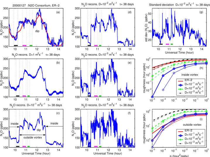
Fig. 6. Reconstructions and roughness for the 27 January 2000 flight. (a): Observed (blue) and REPROBUS (red) N2O. (b–f): N2O

reconstructions forD₌1,0.1,0.01,0.001 and 0.0001 m2s−1atτ₌38 days.(g): Standard deviation of N2O within theNparticles released from each location. (h): Roughness for observed and reconstructed transects as indicated in the legend, and for the flight segment located inside the polar vortex. Thick lines: shift isσ₌3 ppbv; thin lines: shift is 2σ. (i): Same as (h) but for the flight segment outside the polar vortex. Three structures are identified in the figure. The peaks in N2O and O3near 12h are due to a dip of the ER-2 and are removed from roughness analysis.

but it is not always possible to identify such structures, espe-cially when stirring is strong. If we give up this idea, a second way consists in using a statistical measure of the fluctuations as a basis for the comparison. In Legras et al. (2003), com-parisons based on spectra and increment variance have been discussed but these measures are sensitive to the small-scale noise and need to be applied to a pre-filtered signal. Legras et al. also introduced a new measure called the roughness function. We refine here this notion to take into account the small-scale instrumental noise without need to pre-filter the signal.

Our definition of roughness is provided by the following algorithm for a discrete curve described by a list ofKpoints

{xi, yi}with an assumed uncertainty±σ:

1. For each value ofp>0 and for each valuexc=xi,yp+(xi)

is defined as the smallest yc such that the parabola

2p(y₋yc)=(x−xc)2lies entirely above the curve

join-ing the points{xi, yi−σ}.

2. Similarly,y_p−(xi)is defined as the largestyc such that

the inverted parabola, defined by turningpinto−p, lies entirely below the curve joining the points{xi, yi+σ}.

3. The two envelope curves y_p+(xi) and yp−(xi)

are then used to define the roughness function

φ (p)₌_K1 PK_i₌₁max(0, y_p+(xi)−y−p(xi)).

The reason for using a parabolic smoothing function is that arbitrary rescaling of the units of xi and yi preserves

(8)

10 11 12 13 14 0.5

1 1.5 2 2.5 3 3.5

4 20000127 :OZONE PHOTOMETER

O3

(ppmv)

(a)

10 11 12 13 14 0.5

1 1.5 2 2.5 3 3.5 4

O

3 recons. D=1 m

2_s−1_{τ= 38 days}

O3

(ppmv)

(b)

10 11 12 13 14 0.5

1 1.5 2 2.5 3 3.5 4

O

3 recons. D=10 −1

m2s−1 τ= 38 days

O3

(ppmv)

10 11 12 13 14 0.5

1 1.5 2 2.5 3 3.5 4

O₃ recons. D=10−2 m2s−1 τ= 38 days

O3

(ppmv)

(d)

10 11 12 13 14 0.5

1 1.5 2 2.5 3 3.5 4

O

3 recons. D=10

−3_m2_s−1_{τ= 38 days}

O3

(ppmv)

(e)

10 11 12 13 14 0.5

1 1.5 2 2.5 3 3.5 4

O

3 recons. D=10 −4

m2s−1 τ= 38 days

O3

(ppmv)

10 11 12 13 14 0.2

0.4 0.6 0.8 1 1.2

std dev (O

3

) (ppmv)

Standard deviation D=10−2 m2s−1 τ= 38 days

(g)

10−6 10−5 10−4 10−3 10−2 101

102 103

ER−2 D=10−1 m2s−1 D=10−2 m2s−1 D=10−3 m2s−1

10−6 10−5 10−4 10−3 10−2 250

500 1000 2000

p (hour2/ppbv)

ER−2 D=10−1 m2s−1 D=10−2 m2s−1 D=10−3 m2s−1 dip

dip

inside vortex

outside vortex (h)

(i)

Fig. 7.Same as Fig. 6 but for O3andσ=10 ppbv.

both side. The distance between the two envelope curves is then a measure of roughness. We do not want, however, this measure to be dominated by noise at small scale. This is accounted in steps 1 and 2 above by shifting the upper and lower envelope curves, respectively down and up, by the measurement precisionσ, and by calculating the roughness function as a discretized version of the positive area between the two shifted envelope curves. Figure 5 illustrates the al-gorithm for two curves obtained with two values ofD. The dependence of roughness upon scale is described by varying

pwith multiplicative steps. It can be shown that calculating the envelope curves reduces to a Legendre transform which is performed using a fast algorithm (Lucet, 1997).

6 Analysis of SOLVE flights

We first present a detailed analysis of the 27 January 2000 flight which spans both the inside and the outside of the vor-tex and displays a number of interesting structures. Figures 6 and 7 shows the measured and reconstructed transects on 27

January 2000 for both N2O and O3andτ₌38 days, with five values ofDranging from a large valueD₌1 m2_s−1_{, akin to} radar estimates, to the molecular valueD₌10−4_m2_s₋1_.

(9)

the third one (green) is presumably the trace of a filament expelled from the polar vortex. For all these structures, the three smallest values ofD reconstruct excessive amplitude with respect to the observations andD_≈0.1 m2s−1provides a better fit. It is also clear that the edge of the polar vortex is too steep for the three smallest values ofD. Hence, on the edge and outside the polar vortex, the turbulent diffusion must be fairly large to account for the observed structures.

It is more difficult to associate observed and reconstructed structures inside the vortex for timet >13:00 UT but the vi-sual analysis now reveals thatD₌0.1 m2s−1 reconstructs a too smooth transect compared to the observation, suggesting that turbulent diffusion is smaller inside the vortex. Taking this into account, roughness has been calculated separately inside and outside the vortex (removing also the dip section) and also for two different values of the offset, one times and two times the relative precision of measurement. The two families of roughness curves displayed in Figs. 6 and 7 show that the small-scale fluctuations, for both N2O and O3, scale best in agreement withD_≈0.1 m2s−1outside the vortex and withD_≈0.001 m2s−1inside. The inside value, which is in-deed very small, must be tempered by the small length of the branch inside the vortex during this flight.

The 27 January 2000 flight is, however, the only one to ex-hibit a significant level of tracer fluctuations inside the polar vortex. All the 8 flights done entirely within the polar vor-tex exhibit very few tracer fluctuations when the ER-2 flies on level legs (on a slightly climbing trajectory actually), as if the vortex was very well mixed during this winter except for a few minor intrusions (Jost et al., 2002) or anomalous diabatic events. In fact, strong sudden warmings which are the main source of variability within the vortex did not occur during 2000 Arctic winter before mid-March. As a result, the comparison of observed and reconstructed transects is also a test for the transport errors due to the analysed winds used in the reconstruction. Figure 8 compare observed and reconstructed transects for 7 March 2000. Except near the dip, the observed transects for both N2O and O3do not ex-hibit any other structures than small-scale fluctuations over the constant level legs. These fluctuations exceed only occa-sionally the precision for N2O but can be considered as sig-nificant for O3which is measured with better accuracy. It is also visible from the N2O reconstruction that the reconstruc-tion enhances a number of structures at scales larger than 100 km (about 8 min of flight) that are absent from the obser-vations. In particular, a spurious maximum is obtained near 11:00 UT. Through the cascade process of chaotic advection, these structures generate small-scale fluctuations requiring a diffusivityD_≈0.1 m2s−1 to fit the roughness of the obser-vations. The O3 reconstruction does not exhibit the same amount of spurious mesoscale structures as N2O and hence generates less small-scale structures, resulting into a value ofD_≈0.01 m2s−1fitting observed roughness. The spurious structure near 11:00 UT is, however, seen in the standard de-viation. Our interpretation of this discrepancy is that the

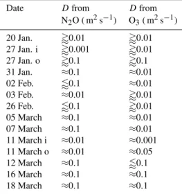
spu-Table 1.Table of estimated Lagrangian diffusivity based on rough-ness curves for the 10 processed flights of the campaign and the return flights of 16 and 18 March. The two flights of 27 January 2000 and 11 March 2000 have been split into legs inside (i) and outside (o) the polar vortex. All the other flights between 20 Jan-uary and 12 March are inside the polar vortex. The two flights on 16 and 18 March are within the surf zone.

Date Dfrom Dfrom

N2O ( m2s−1) O3( m2s−1)

20 Jan. '0.01 '0.01 27 Jan. i '0.001 '0.01 27 Jan. o '0.1 '0.1 31 Jan. _≈0.1 _≈0.01 02 Feb. /0.1 _≈0.01 03 Feb. _≈0.01 '0.01 26 Feb. /0.1 '0.01 05 March _≈0.1 _≈0.01 07 March _≈0.1 _≈0.01 11 March i _≈0.01 _≈0.001 11 March o _≈0.01 _≈0.05 12 March _≈0.1 /0.1 16 March _≈0.1 _≈0.1 18 March _≈0.1 _≈0.1

rious structures in the N2O reconstruction are due to spuri-ous vertical transport in the vertical N2O gradient and that the lower sensitivity of O3is due to its weaker vertical gra-dient measured by the height-scale_[O3_]∂p/∂_[O3_]≈128 hPa compared to 56 hPa for N2O at 60 hPa inside the polar vortex in early March. It is worth noticing that the reconstruction tends to generate less spurious structures than REPROBUS itself; this result might be due to the fact that REPROBUS uses 6-hourly analysed winds while our reconstructions are based on 3-hourly winds (see Sect. 9 below). There are also indications that we are able to reconstruct the small maxi-mum denoted as E in Fig. 8, just before the dip, which has been identified as an intrusion of mid-latitude air by Jost et al. (2002) and Konopka et al. (2004).

Table 1 summarizes the estimates ofD based on rough-ness for N2O and O3, and checked by visual inspection, for all the flights of the SOLVE campaign from Kiruna. It is ap-parent that previous results are mostly confirmed during the whole campaign with the noticeable exception of 11 March 2000 flight during which fairly small diffusion was observed outside the polar vortex in the N2O reconstructions.

(10)

8 10 12 14 50 100 150 200 250

20000307 :N2O Consortium

N2

O (ppbv)

(a)

8 10 12 14 50 100 150 200 250 N

2O recons. D=0.1 m 2_s−1

N2

O (ppbv)

(d)

8 10 12 14 50 100 150 200 250 N

2O recons. D=0.01 m 2_s−1

N2

O (ppbv)

(e)

8 10 12 14 50

100 150 200 250

N₂O recons. D=0.001 m2s−1

N2

O (ppbv)

8 10 12 14 10

20 30 40

std dev (N

2

O) (ppbv)

Standard deviation D=0.01 m2s−1

(b)

10−5 10−4 10−3 10−2 10−1 100 10−4

10−2 100 102

p (hour2/ppbv)

ER−2 D=10−1 m2s−1 D=10−2 m2s−1 D=10−3 m2s−1

8 10 12 14 1

1.5 2 2.5 3

3.5 20000307 :OZONE

O 3

(ppmv)

(g)

8 10 12 14 1 1.5 2 2.5 3 3.5

O₃ recons. D=0.1 m2s−1

O3

(ppmv)

(j)

8 10 12 14 1 1.5 2 2.5 3 3.5 O

3 recons. D=0.01 m 2_s−1

O3

(ppmv)

(k)

8 10 12 14 1 1.5 2 2.5 3 3.5 O

3 recons. D=0.001 m 2_s−1

O3

(ppmv)

Universal Time (hour) (l)

8 10 12 14 0.05 0.1 0.15 0.2 0.25 0.3

std dev (O

3

) (ppmv)

(h)

10−6 10−5 10−4 10−3 10−2 100

101 102 103

p (hour2/ppbv)

(i)

ER−2 D=10−1 m2s−1 D=10−2 m2s−1 D=10−3 m2s−1 (c)

dip dip dip

dip

E

E E

E

Fig. 8.Reconstructions and roughness for the 07 March 2000 flight inside the polar vortex. Left six panels for N2O and right six panels for O3.(a): Observed (blue) and REPROBUS (red) N2O.(d, e, f): N2O reconstructions forD=0.1, 0.01 and 0.001 m2s−1atτ=34 days.(b): Standard deviation of N2O among theNparticles released from each location. (c): Roughness for observed and reconstructed transects as indicated in the legend. Thick lines: shift isσ₌3 ppbv; thin lines: shift is 2σ.(g–l): Same as (a–h) but for O3andσ=10 ppbv.

7 Local variations of turbulent diffusion

As already noticed in Section 4, the 11 March 2000 flight crossed a sheet of polar air at some distance outside the vor-tex edge. This sheet is the remain of a fairly broad streamer emitted from the vortex by 28 February 2000, 13 days earlier. On 11 March, its signature was very faint in the ECMWF analysed potential vorticity (not shown) but it was still very well preserved in the N2O field. Its weak signature in the O3 field is due to the weak horizontal O3gradient in the region where it originates from.

Figure 10 shows an enlargement of the sheet crossing for the observed and reconstructed transects. The flight was mainly along mean tracer gradients and the observed sheet was met 325 km after crossing the vortex edge. The sheet is 120 km large and the striking feature is the asymmetry of its two edges. The south edge is smooth and fits very well an error function with width 32 km. The north edge is steep with a width of about 2.5 km. The reconstruction succeeds in reproducing the sheet albeit it is slightly displaced south-ward by 104 km but the asymmetry of the sheet cannot be reproduced with a single value of the diffusivity which gen-erates the same slope on both edges. The observed south slope of 1.49 ppbv km−1 lies between that forD₌0.1 and

0.01 m2s−1, respectively 1.22 and 2.64 ppbv km−1, closer to the first one. The observed north slope is as steep as that for

D₌0.001 m2s−1. Hence, a variation of more than one order of magnitude for the Lagrangian turbulent diffusion occurs over a short distance of about 100 km across the sheet.

It would not be surprising to observe such variations in the instantaneous turbulent diffusion which is expected to be very intermittent in time and space, but the persistence of sharp variations in the averaged Lagrangian diffusivity indi-cates the presence of a transport barrier. Noting that large fluctuations, compatible with low diffusion, are observed be-tween the filament and the vortex edge, it is tempting to sug-gest that the dynamical vortex edge does not coincide in this case with the chemical edge but is located right in the center of the sheet.

8 Relation between diffusion and dispersion

(11)

8 10 12 14 180

200 220 240 260 280

300 20000316 :N2O Consortium

N2

O (ppbv)

(a)

8 10 12 14 180

200 220 240 260 280 300

N2

O (ppbv)

(d)

8 10 12 14 180

200 220 240 260 280 300

N2

O (ppbv)

(e)

8 10 12 14 180

200 220 240 260 280 300

N2

O (ppbv)

Universal Time (hour) (f) 8 10 12 14

10 20 30 40

std dev (N

2

O) (ppbv)

(b)

10−5 10−4 10−3 10−2 10−1 100 100

102

p (hour2/ppbv)

ER−2 D=10−1 m2s−1 D=10−2 m2s−1 D=10−3 m2s−1

8 10 12 14 0

1 2 3

4 20000316 :OZONE

O3

(ppmv)

(g)

8 10 12 14 0

1 2 3 4

O3

(ppmv)

(j)

8 10 12 14 0

1 2 3 4

O3

(ppmv)

(k)

8 10 12 14 0

1 2 3 4

O3

(ppmv)

Universal Time (hour) (l)

8 10 12 14 0.2

0.4 0.6 0.8 1

std dev (O

3

) (ppmv)

10−6 10−5 10−4 10−3 10−2 103

104

p (hour2/ppbv)

ER−2 D=10−1 m2s−1 D=10−2 m2s−1 D=10−3 m2s−1 (c)

(h)

(i)

Fig. 9.Same as Fig. 8 but for the 16 March 2000 flight outside the polar vortex andτ₌29 days.

9.2 9.4 9.6 9.8 10 100

150 200 250

20000311 :N2O Consortium, ER−2

N2

O (ppbv)

9.2 9.4 9.6 9.8 10 100

150 200 250

N

2O recons. D=0.1 m

2_s−1_τ_{= 32 days}

N2

O (ppbv)

9.2 9.4 9.6 9.8 10 100

150 200 250

N

2O recons. D=0.01 m

2_s−1_τ_{= 32 days}

N2

O (ppbv)

9.2 9.4 9.6 9.8 10 100

150 200 250

N

2O recons. D=0.001 m

2_s−1_τ_{= 32 days}

N2

O (ppbv)

Universal Tme (hour) (a)

(b)

(c)

(12)

50 100 150 200 250 300 350 400 450 500 −20

−15 −10 −5 0 5

Time (hour)

log

10

(inertial volume (km

3))

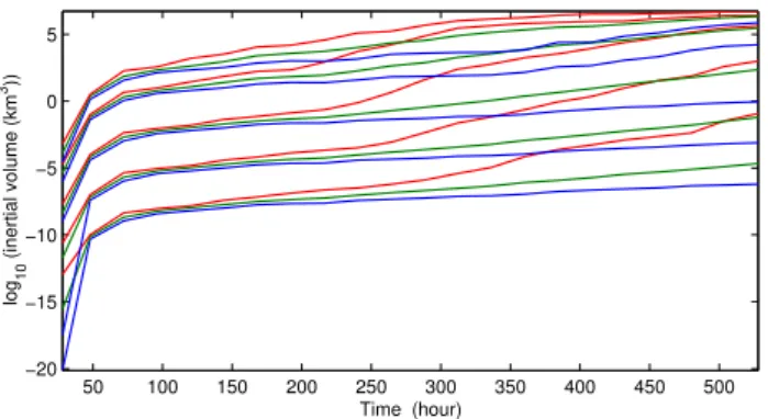
Fig. 11.Inertial volume calculated for the cloud ofNparticles emit-ted from the flight track every 4 seconds. The inertial volume is calculated by diagonalizing the inertia matrix of the cloud and tak-ing the square-root of the product of the diagonal terms. Families of curves from bottom to top: D₌10−8m2s−1 D₌10−6m2s−1 D₌10−4m2s−1 D₌10−2m2s−1 D₌10−1m2s−1. Green: av-erage log(volume); blue: 5% percentile of the distribution; red: 95% of the distribution. The distribution consists in 500 points over a selected 2000 s section of the 27 January 2000 flight.

2004), mixing is parametrized as a function of the deforma-tion of a grid of points advected by the flow.

Since turbulent diffusion is estimated here independently of any relation with dispersion, it is interesting to compare both quantities.

8.1 Onset of dispersion

First we check the consistency of our numerical calcula-tions with respect to the dynamics of advection and diffusion. Starting from a spatialδ-distribution, diffusion initially dom-inates and the inertial axis of the cloud ofNparticles grow as

D1/2t1/2. This applies here to all axes even if diffusion only acts in the vertical direction because the time stepδt is such that3δt₌O(1). This first stage ends when the cloud reaches a sizeℓd≈D1/2γ−1/2 for which diffusion equilibrates with

strain in one direction, after which expansion of the cloud pursues exponentially with a rate of the orderγ as a pancake or a filament (depending on the number of unstable direc-tions) while the smaller transverse dispersion remains of the order ofℓd.

The duration t∗ of the first stage satisfies D1/2t∗1/2 _∼ D1/2γ−1/2 and hence should be independent ofD. This is checked in Fig. 11 showing the growth of the inertial volume for a wide range of diffusivity values, including unrealistic sub-molecular values. The diffusive stage for all cases ends at the samet∗_≈3 days. The subsequent growth rate of the in-ertial volume is bounded by two curves showing the 5% and 95% percentiles of the distribution. The growth is exponen-tial as long as the largest size of the cloud remains small with respect to the characteristic scale of strain variation and the cloud retains an ellipsoidal shape. This linearity condition is more easily satisfied for the 5% percentile which corresponds

to a growth rate of 0.26 days−1_{. The upper 95% percentile} grows initially at a higher rate of 0.63 days−1. For the two largest diffusions tested here, the size of the cloud rapidly vi-olates the linearity condition and the growth weakens as the cloud distorts and mixes with itself.

8.2 Lyapunov exponents

A geometric measure of deformation induced by strain is provided by the Lyapunov exponents (Pierrehumbert and Yang, 1993). For non diffusive motion, they describe the transformation of an infinitesimal spherical cloud surround-ing a particle at timet0 into an ellipsoid at timet1in a lo-cal reference frame relative to the particle. If δx(t )is an infinitesimal deviation at time t, its evolution is described by the tangent linear operatorMasδx(t1)=M(t0, t1)δx(t0) and the local finite-time Lyapunov exponentsλi are related

to the eigenvaluesσi ofMtMby 2λi=1/(t1−t0)lnσi where

superscripttdenotes transposition. A convenient way to cal-culate the local Lyapunov exponents is by finite difference using a small initial perturbation in three orthogonal direc-tions and performing, at regular intervals, an estimate of the growth of length, surface and volume, followed by an ortho-normalization procedure that regenerates an initial trihedron for the following interval (for more details, see Benettin et al. (1980); Ott (1993)). It can be shown (Goldhirsch et al., 1987) that, after a transient time, this method provides the three lo-cal Lyapunov exponentsλ1≧λ2≧λ3. SinceMcan be calcu-lated as a by-product of the procedure for short times, it has been checked that this is true fort1−t0>20 days. The norm used in the orthogonalization takes into account the aspect ratio of stratospheric structures by magnifying the vertical di-rection by a factorαwith respect to the horizontal directions. Doing so, we define a distance in terms of tracer difference rather than in terms of metric separation. Although infinite time Lyapunov exponents are independent on the norm, fi-nite time exponents and convergence to the large time limit depend on it. The Lyapunov exponents are calculated over the durationτ(that isτ₌t1−t0) near the single trajectory ob-tained forD₌0 and the orthogonalization interval is one day. For backward evolution in time, the smallest exponentλ3 describes the exponential elongation of line segments, while

λ1+λ2 describes the growth rate of surface elements and

λ1+λ2+λ3describes the growth rate of the volume. Since the flow is close to incompressible, the sum of the three ex-ponents should be close to zero. Three cases can hold:

1. λ1≈λ2>0, λ3≈−λ1−λ2 which means that sheets are formed ift >0 and filaments ifτ <0.

2. λ1>0 and λ2≈λ3<0 which means that sheets are formed ift <0 and filaments ifτ >0

(13)

9 10 11 12 13 14 15 50

100 150 200 250 300

N₂O recons. D=0.01 m2s−1 τ= 32 days

N2

O (ppbv)

9 10 11 12 13 14 15 10

20 30 40 50 60

Standard deviation D=0.01 m2s−1 τ= 32 days

std dev (N

2

O) (ppbv)

9 10 11 12 13 14 15 −0.5

0 0.5

Lyapunov exponents for τ = 32 days

FTLE (day

−1

)

(a)

(b)

(c)

Fig. 12. (a)N2O reconstruction for the 11 March 2000 flight with D₌0.01 m2s−1 andτ₌32 days. (b) N₂O standard deviation of theNparticles within each diffusive ensemble. (c)Lyapunov ex-ponents, blue:λ1, green: λ2, red: λ3, black: λ1+λ2+λ3. The location of the polar air sheet crossings is outlined.

For diffusive motion and backward in time, the negative exponents describe the elongation of the cloud of particles emitted from each point for|τ_|>t∗.

Figure 12 shows the N2O reconstruction and Lyapunov exponent for 11 March 2000 and τ₌32 days. Since the calculation is based on single deterministic trajectories, the Lyapunov exponents are noisy but several properties can be drawn from the figure. There is a clear separation in mag-nitude between the inside of the polar vortex, with typical values smaller than 0.1 day−1and small tracer standard de-viation, and the outside, with typical values of the order of 0.25 day−1 and large tracer standard deviation. Hence, the inside of the polar vortex is much less strained than the out-side. This is in agreement with previous studies of the winter polar stratosphere (Pierce and Fairlie, 1993; Bowman, 1993). Larger dispersion, especially in the vertical, means sampling a wider range of N2O values, and the tracer standard devia-tion is also larger outside the polar vortex than inside. The unfiltered curves of the most negative Lyapunov exponent and the standard deviation are anti-correlated with a coeffi-cient−0.407 which is significant since it is calculated over 8844 points along the flight. The sum of the three Lyapunov exponents is close to zero. In principle, its variation should correlate with the variation of parcel density which can be

9.2 9.4 9.6 9.8 10 50

100 150 200 250 300

N₂O recons. D=0.01 m2s−1 τ= 32 days

N2

O (ppbv)

9.2 9.4 9.6 9.8 10 10

20 30 40 50 60

Standard deviation D=0.01 m2s−1 τ= 32 days

std dev (N

2

O) (ppbv)

9.2 9.4 9.6 9.8 10 −0.5

0 0.5

Lyapunov exponents for τ = 32 days

FTLE (day

−1

)

(a)

(b)

(c)

Fig. 13. Enlargement of Fig. 12 encompassing the first crossing of the polar air sheet.

calculated, but we reach here the limit of our numerics and the correlation is very poor. The sign of the intermediate Lyapunov exponent oscillates around 0 along the flight but its magnitude is always much smaller than the two large negative and positive exponents which almost compensate. Hence, we are essentially in the third case defined above.

Figure 13 shows an enlargement around the sheet of polar air. The small dispersion that characterizes the polar air has been preserved inside the sheet in agreement with its isola-tion from surrounding air. Both edges exhibit a maximum, indicating that strong shear, presumably due to PV jump, has been experienced by the parcels over the last three weeks but there is no distinction between the smooth and the sharp edge. This suggests that the event that led to the smooth south edge is not due to shear induced turbulence but rather to an exterior event such as breaking gravity waves, not unlikely to occur along the cost of Scandinavia.

9 Sensitivity to temporal resolution

(14)

9 10 11 12 13 14 15 50

100 150 200 250

300 20000311 :N2O Consortium, ER−2

N 2

O (ppbv)

ER−2 N₂O REPROBUS

9 10 11 12 13 14 15 50

100 150 200 250

300 std analysis + fcst, 1 degree & 3 hours

N 2

O (ppbv)

9 10 11 12 13 14 15 50

100 150 200 250

300std analysis + fcst, 1/2 degree & 3 hours

N2

O (ppbv)

9 10 11 12 13 14 15 50

100 150 200 250

300 std analysis, 1 degree & 6 hours

N2

O (ppbv)

9 10 11 12 13 14 15 50

100 150 200 250

300 2−day forecast, 1 degree & 6 hours

N2

O (ppbv)

9 10 11 12 13 14 15 50

100 150 200 250

300 ERA40, 1 degree & 3 hours

N2

O (ppbv)

Universal Time (hour) (a)

(b)

(c)

(d)

(e)

(f)

Fig. 14. Comparison of observed N2O and reconstructions for different resolutions of the advecting wind. (a) Observed N2O and

REPROBUS prediction. (b): Reconstructed N2O using 3-hourly analysed and first guess winds on a 1◦latitude-longitude grid which is the standard setting for all other figures. (c): Same as (b) but using winds on a 0.5◦grid. (d): Same as (b) but using only the 6-hourly analysed winds. (e): Same as (d) but replacing the analysed winds by 6-hourly forecast winds generated twice-daily from the 48 and 54 hours forecasts. (f): Same as (b) but using the ERA-40 reanalysis instead of the operational analysis. All reconstructions are done with D₌0.01 m2s−1andτ₌32 days.

implemented in FLEXPART (Stohl et al., 2002) and inher-ited in TRACZILLA. A number of other Lagrangian stud-ies in the literature have used instead 6-hourly winds based solely on analysis. The main reason for this choice seems practical since the ECMWF 6-hourly analysis or re-analysis are mirrored and easily available from many locations. It is, however, questionable that the 6-hour archiving period, which has been chosen to provide accurate climatology, is optimum to perform off-line transport calculations. This led us to investigate the effect of changing the temporal resolu-tion of advecting winds onto the reconstrucresolu-tion and estimated turbulent diffusion. An other motivation was a recent work (Stohl et al., 2004) showing that forecasted winds are much less diffusive than analysis. Hence, we have also tested the effect of replacing analysed winds by forecasted winds.

We have performed a series of reconstructions for the same case, namely that of 11 March 2000 which is already well documented in this study, and for a single value of diffusiv-ityD₌0.01 m2s−1by varying the field of advecting winds. The reference reconstruction, shown in Fig. 14b is that per-formed with 3-hourly winds, one-degree horizontal resolu-tion and 60 hybrid levels in the vertical. Figure 14c shows the reconstruction obtained by halving the horizontal resolution of advecting winds to 0.5◦. The reconstruction is strikingly insensitive to this spatial refinement in agreement with pre-vious observations (Waugh and Plumb, 1994; Methven and

Hoskins, 1999) and the fact that ECMWF analysed winds bear little variance at such small scales in the lower strato-sphere. Notice also that near the pole the 1◦_{longitude-latitude}

(15)

These results indicate that off-line transport calculations are highly sensitive to the lack of resolution of the wind fluc-tuations in 6-hourly analysis. Flucfluc-tuations are mostly seen in the vertical wind calculated from the divergence field, no-toriously noisy in the analysis, using the mass conservation. Whatever the true timescale of a given fluctuation, sampling the wind field everyxhours makes it persistent overxhours. As a result, vertical displacements are overestimated and in turn, eddy transport along vertical tracer gradients is also overestimated. In the limit of very short-lived fluctuations, it can be shown easily that vertical eddy transport is propor-tional to the sampling interval. For our prospect of measuring turbulent diffusion, the excess transport leads to overestimate Lagrangian diffusion in order to smooth out the excess fluc-tuations in the reconstructed tracer.

Not only the fluctuations in the 6-hourly winds are under-sampled, they are also to a large extend spurious as demon-strated from the comparison between analysed and forecast winds. In spite of the efforts to filter out gravity waves during assimilation, the analysed winds contain a significant level of spurious motion which is damped during the forecast as the model relaxes to its attractor (Kalnay, 2003). This spurious motion presumably consists mainly in short-period gravity waves. Wavy structures with scales of the order of several tens to a few hundreds km are often seen over the displace-ments of the cloud of parcels emitted from a single location or even in the reconstruction itself. Figure 15 shows such an example.

However, it is still unclear whether 3 h (the maximum fre-quency at which wind datasets are currently available) is a sufficiently short interval to achieve satisfying reconstruc-tions. In fact, the discrepancy between estimates ofDfrom N2O and O3 inside the vortex suggests that this is not the case and that our estimate ofDis still an upper bound of the true value representing unresolved turbulent motion.

10 Conclusions

We have shown that the sensitivity of Lagrangian reconstruc-tion to the integrareconstruc-tion time of back-trajectories disappears when diffusion is added as a random walk over an ensem-ble of trajectories and reconstruction is based on statistical average over this ensemble. Using the tracer field produced by REPROBUS as initialisation, it takes 2 to 4 weeks for diffusivity varying from 0.1 m2s−1to 0.001 m2s−1to reach a stage where small-scale structures are essentially invariant under extension of the reconstruction time.

The comparison of ER-2 measurements of N2O and O3 with reconstructions performed with varying diffusivity pro-vides an estimate of turbulent diffusivity of the order of 0.1 m2s−1in the surf zone and one order of magnitude less, at least, inside the polar vortex, based on the statistical dis-tribution of tracer fluctuations. When well-defined structures are identified in the observations and the reconstructions, a

−1000 0

1000

−1500 −1000 −500 0 500 1000 −0.7 −0.6 −0.5 −0.4 −0.3 −0.2 −0.1 0 0.1 0.2 0.3

x (km) Parcel 31 cloud at τ = 22 days

y (km)

z (km)

Fig. 15. Distribution of the cloud of points at τ₌22 days for a parcel along the 11 March 2000 flight track. Calculation is done withD₌10−4m2s−1in order to reduce lateral dispersion and to magnify the wavy pattern. It can be checked that dispersion occurs as a filament.

local estimate of diffusivity is possible, and large variations of more than one order of magnitude have been observed across the width of a polar vortex sheet.

The dispersion measured by Lyapunov exponent is much reduced inside the polar vortex compared to outside. There-fore, models that parametrize mixing based on deformation, like CLAMS (Konopka et al., 2004) would correctly predict less mixing inside the polar vortex than outside. However, the absence of correlation between diffusion and dispersion on the two edges of the polar air sheet on 11 March 2000 is an indication that such parametrization may miss numerous mesoscale features.

The estimate of diffusivity within the surf zone is in agree-ment with previous results based on ozone sounding (Legras et al., 2003). The resolution of standard ozone soundings is so coarse that lower diffusivity could not be tested while the ER-2 data are providing a much higher resolution and are much better suited to study the small-scale fluctuations of tracers.

(16)

14 15 16 17 18 19 20 50

100 150 200 250

300 19920104 :ATLAS

N2

O (ppbv)

14 15 16 17 18 19 20 50

100 150 200 250 300

N

2O recons. D=0.1 m

2_{/s τ=35 days}

N2

O (ppbv)

14 15 16 17 18 19 20 50

100 150 200 250 300

N

2O recons. D=0.01 m

2_{/s τ=35 days}

N2

O (ppbv)

Universal Time (hour) 15.2 15.4 15.6 15.8 16 16.2

50 100 150 200 250

N₂O recons.: zoom on vortex edge

N2

O (ppbv)

Universal Time (hour) ER−2 D=0.1 m2/s D=0.01 m2/s

10−4 10−2 100 100

101 102

ER−2 D=0.1 m2/s D=0.01 m2/s

10−4 10−2 100 100

102

p (hour2/ppbv)

ER−2 D=0.1 m2/s D=0.01 m2/s (a)

(b)

(c)

(d)

(e)

(f)

inside vortex

outside vortex dip

dip

inside vortex outside

vortex

outside vortex

Fig. 16. N2O reconstruction for the 4 January 1992 flight during AASEII campaign in the Arctic. (a): Measured N2O along the flight track.(b): Enlargement of the observed and reconstructed curves near the vortex edge.(c–d): N₂O reconstruction withD₌0.1 m2s−1and 0.01 m2s−1. (e): Roughness of observed and reconstructed transects for the flight segments inside the polar vortex. (f): Roughness of observed and reconstructed transects for the flight segments outside the polar vortex

14 15 16 17 18 19 20 0

50 100 150 200 250

300 19920108 :ATLAS

N2

O (ppbv)

14 15 16 17 18 19 20 0

50 100 150 200 250 300

N

2O recons. D=0.1 m

2_{/s τ=39 days}

N2

O (ppbv)

14 15 16 17 18 19 20 0

50 100 150 200 250 300

N

2O recons. D=0.01 m

2_{/s τ=39 days}

N 2

O (ppbv)

Universal Tme (hour) dip dip

A

A C

C

C B

B D

D _B _D

E

E dip dip

(a) _(b) _(c)

Fig. 17.N2O reconstruction for the 8 January 1992 flight during AASEII campaign in the Arctic.(a): Measured N2O along the flight track.

(b–c): N2O reconstruction withD=0.1 m2s−1and 0.01 m2s−1.

are too low by almost 40% but the variations are fairly well reproduced. Like during SOLVE, there is a large contrast in turbulent diffusion between the inside and the outside of the vortex, with non ambiguous indication ofD_≈0.1 m2s−1 rather than 0.01 m2s−1outside the vortex. Figure 16b is an enlargement of the vortex edge corresponding to Fig. 9 of Balluch and Haynes (1997), showing that the observed N2O agrees better with our large diffusion rather than with the small value. Among the two other cases studied by Balluch and Haynes (1997), the sheet is entirely missed in our re-construction of 7 May 1993 flight due to the very short track and Fig. 17 shows the reconstructions of the 8 January 1992

(17)

with Balluch and Haynes (1997) and Waugh et al. (1997). These studies were based on a very small amount of data and it is quite possible that they sampled domains of small diffu-sion around the polar vortex. The sample of cases outside the polar vortex is also limited in the SOLVE campaign, and fur-ther studies are required to establish the spatial and temporal variations of turbulent diffusion in the lower stratosphere.

The reconstructions are found to be sensitive to the quality of the wind fields used for the advection. In particular, the ECMWF analysis seems to contain a significant amount of short-lived fluctuations which induce spurious transport, es-pecially if advecting winds are interpolated between 6-hourly standard ECMWF archived winds.

This spurious effect is probably also affecting transport in REPROBUS. For instance the overestimation of N2O within the polar vortex on 11 March 2000 (see Fig. 3) is also found in the CLAMS model when mixing is set at a too high value (Konopka et al., 2004, Fig. 8). Our reconstruc-tion based on 3-hourly winds reduces the spurious mixing and hence decreases the value of N2O towards the observed value. The fact that slightly lower values than observed are obtained in Fig. 3(i) could be attributed to errors in the initial REPROBUS field or too strong diabatic descent within the vortex.

The turbulent diffusivity estimated in this study is the com-bination of the unresolved turbulent motion (the “true turbu-lent diffusivity”) and the diffusion required to filter out the structures induced by the spurious motion contained in the analysed winds. The second effect is likely to hinder the first one as suggested by the comparison of results obtained with N2O and O3. It is also possible that chemical reactions contribute to smooth the spatial fluctuations of O3 but it is not easy to conceive a possible mechanism since depletion chemistry does not tend to relax O3to an equilibrium value and ClO fluctuations should rather increase the ozone fluctu-ations (Edouard et al., 1996).

Our results indicate that the state-of-the-art in off-line transport studies, which is mainly based on 6-hourly anal-ysed winds, is far from being satisfactory. A significant im-provement is provided by interleaving first guesses to provide 3-hourly winds but it is yet unclear that these winds do not contain significant signature of high-frequency fluctuations as aliases, and hence are still inducing excess transport with respect to what would be found by performing on-line cal-culations. This latter solution does not seem practical with an operational weather forecast model but archiving winds at higher resolution could be considered, at least for test purpose over a limited period of time. Another possibility would be to archive time-averaged winds instead of instan-taneous snapshots. The fact that the high frequency fluctua-tions are to some large extend a spurious effect of the assim-ilation could be perhaps circumvented by using winds from short-time forecast, as suggested by the strong improvement shown in Fig. 14e. Finally, a number of models, including CLAMS, are using in the stratosphere vertical winds

calcu-lated from the local heating rate and the vertical profile of po-tential temperature. Although such winds are not providing automatic mass conservation they seem to reconstruct better the observed tracer, at least in Fig.12 of Konopka et al. (2004) for 07 March 2000. These questions will be investigated in further work.

Acknowledgements. We acknowledge D. F. Hurst, H.-J. Jost, E. C.

Richards, C. R. Webster, J. W. Elkins, S. M.. Schauffler and E. L. Atlas for provided data from ACATS, ARGUS, ALIAS, WAS and ozone instruments on board the ER-2 during the SOLVE cam-paign. We acknowledge A. Tuck for useful discussions and advices.

Edited by: P. Haynes

References

Alisse, J.-R., Haynes, P., Vanneste, J., and Sidi, C.: Quantification of stratospheric mixing from turbulence microstructure measure-ments, Geophys. Res. Lett., 27, 2621–2624, 2000.

Appenzeller, C., Davies, H., and Norton, W.: Fragmentation of stratospheric intrusions, J. Geophys. Res., 101, 1453–1456, 1996.

Balluch, M. and Haynes, P.: Quantification of lower stratospheric mixing processes using aircraft data, J. Geophys. Res., 102, 23 487–23 504, (97JD00 607), 1997.

Benettin, G., Galgani, L., Giagilli, A., and Strelcyn, J.-M.: Lya-punov characteristic exponents for smooth dynamical systems and for Hamiltonian systems; a method for computing all of them. I: Theory, Meccanica, pp. 9–80, 1980.

Bowman, K. P.: Large-Scale Isentropic Mixing Proprieties of the Antarctic Polar Vortex From Analyzed Winds, J. Geophys. Res., 98, 23,013–23,027, 1993.

Edouard, S., Legras, B., Lef`evre, F., and Eymard, R.: The effect of small-scale inhomogeneities on ozone depletion in the Arctic., Nature, 384, 444–447, 1996.

Falkovich, G., Gawe¸dski, K., and Vergassola, M.: Particles and fields in fluid turbulence, Rev. Mod. Phys., 73, 913–975, 2001. Fukao, S., Yamanaka, M., Ao, N., Hocking, W., Sato, T.,

Ya-mamoto, M., Nakamura, T., Tsuda, T., and Kato, S.: Seasonal variability of vertical eddy diffusivity in the middle atmosphere. Three-year observations by the middle and upper atmosphere radar, J. Geophys. Res., 99, 18 973–18 987, 1994.

Goldhirsch, I., Sulem, P.-L., and Orszag, S. A.: Stability and Lya-punov stability of dynamical systems: a differential approach and a numerical method, Physica D, 27, 311–337, 1987.

Haynes, P. and Anglade, J.: The vertical-scale cascade of atmo-spheric tracers due to large-scale differential advection, J. Atmos. Sci., 54, 1121–1136, 1997.

Haynes, P. and Vanneste, J.: Stratospheric tracer spectra, J. Atmos. Sci., 61, 161–178, 2004.

Holzer, M. and Hall, T.: Transit-time tracer-edge distributions in geophysical flows, J. Atmos. Sci., 57, 3539–3558, 2000. Hurst, D., Schauffler, S., Greenblatt, J., Jost, H., Herman, R.,