Annales
Geophysicae
First results of electric field and density observations by Cluster
EFW based on initial months of operation
G. Gustafsson1, M. Andr´e1, T. Carozzi1, A. I. Eriksson1, C.-G. F¨althammar4, R. Grard5, G. Holmgren8, J. A. Holtet3, N. Ivchenko4, T. Karlsson4, Y. Khotyaintsev1, S. Klimov6, H. Laakso5, P.-A. Lindqvist4, B. Lybekk3, G. Marklund4, F. Mozer2, K. Mursula7, A. Pedersen3, B. Popielawska9, S. Savin6, K. Stasiewicz1, P. Tanskanen7, A. Vaivads1, and
J-E. Wahlund1
1Swedish Institute of Space Physics, Uppsala Division, Uppsala, Sweden 2Space Sciences Laboratory, Berkeley, USA
3University of Oslo, Norway
4Alfv´en Laboratory, Stockholm, Sweden
5Space Science Department, ESTEC, Noordwijk, The Netherlands 6Space Research Institute, Moscow, Russia
7University of Oulu, Finland 8University of Uppsala, Sweden
9Space Research Centre, Warsaw, Poland
Received: 11 April 2001 – Revised: 3 July 2001 – Accepted: 6 July 2001
Abstract. Highlights are presented from studies of the
electric field data from various regions along the CLUS-TER orbit. They all point towards a very high coherence for phenomena recorded on four spacecraft that are sepa-rated by a few hundred kilometers for structures over the whole range of apparent frequencies from 1 mHz to 9 kHz. This presents completely new opportunities to study spatial-temporal plasma phenomena from the magnetosphere out to the solar wind. A new probe environment was con-structed for the CLUSTER electric field experiment that now produces data of unprecedented quality. Determination of plasma flow in the solar wind is an example of the capability of the instrument.
Key words. Magnetospheric physics (electric fields) –
Space plasma physics (electrostatic structures; turbulence)
1 Introduction
With its four-point measurements, Cluster is uniquely well adapted to study the small-scale plasma structures in space and time in key plasma regions. To fully utilize this opportu-nity, the Cluster Electric Field and Wave (EFW) instrument has been designed for detailed study of phenomena on spatial scales corresponding to the separation distance of the four spacecraft and their interpretation in terms of the role they play on a more global scale in shaping the properties of dif-ferent regions along the orbit. Combined with the rigorous Correspondence to:G. Gustafsson
pre-launch testing and calibration programme, the novel de-sign of the probe environment enables EFW to measure elec-tric fields with sensitivity that is unprecedented in this region of space. In this paper, we present some of the first results from EFW and show some of the unique features of this in-strument. EFW data are also analysed and presented in other papers in this issue (Andr´e et al., 2001; Pedersen et al., 2001). EFW uses two pairs of spherical probes deployed on wire booms in the spin plane to measure the electric field (Gustafs-son et al., 1997). The probe-to-probe separation is 88 m. We also use measurements of the potential of the spherical probes to the spacecraft, which is a measure of the plasma density (Pedersen et al., 1995; Pedersen et al., 2001 this issue). Data from the fluxgate magnetometer are used to support the analysis of the electric field data (Balogh et al., 1997).
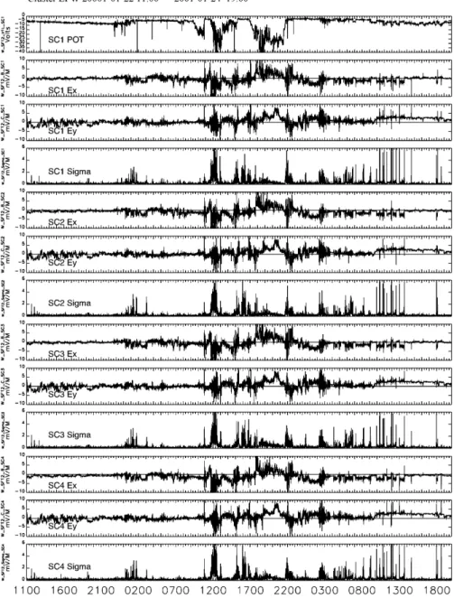
To demonstrate the overall similarity between recordings from the four spacecraft, the electric field and density obser-vations for a full orbit (57 h) are shown in Fig. 1. It is clear from the figure that signals from the four spacecraft look very similar on this time scale. Perigee is located at the center of the panels at 15:50 UT, 23 January 2001 and apogee is near the beginning and end of the panels. The local time of apogee was approximately 14:30 LT.
Fig. 1. A full orbit (57 hours) of EFW data from 22 January, 11:00 UT to 24 January, 19:00 UT. “Pot” is the probe-to-spacecraft voltage, while the other parameters are spin-period averages. EXandEY are the electric field components in the directions of the projections of
the GSEXandY axes in the spin-plane, deviating a few degrees from the true GSEXY plane, while “Sigma” is the RMS deviation of the spin-fits, thus providing information about variations above the spin frequency. The figure shows raw data from onboard processing and a few glitches can be seen in the data.
produced by EFW.
The electron density and gradient of electron density are fundamental parameters where EFW can routinely produce spacecraft potential data with a time resolution of 0.2 s. These data can be related to the electron density with good precision (Escoubet et al., 1997; Pedersen et al., 1995). A preliminary calibration curve for the Cluster instruments for this relation is discussed in Sect. 3.
Electric field waveforms with frequencies below the spin frequency (250 mHz), in many cases, show very close simi-larities between the four Cluster spacecraft in several of the
plasma regions along the Cluster orbit. This opens the possi-bility for in depth studies of the structures. A few examples of structures with very high coherence (0.90 to 0.95) between the four spacecraft are discussed in Sect. 4.
Crossings of auroral field lines by Cluster show high am-plitude electric field variations. Fields of 100 mV/m have been seen that correspond to 1 V/m in the ionosphere. A case of a convergent electric field was identified with a steep plasma density gradient. This case suggests an upward con-tinuation of the quasi-static U-shaped potential which is as-sociated with auroral arcs, as discussed in Sect. 6.
Data from the Cluster instruments offer tremendous pos-sibilities for studying the magnetopause. In Sect. 7, a few examples of waves near the magnetopause are discussed pri-marily based on electric field data. Waves in the lower hybrid range of frequencies (approximately 10 Hz) are suggested to be important for diffusion across the magnetopause and for onset of the reconnection. An event from the dawn side mag-netopause is demonstrated. Kinetic Alfv´en and drift waves are also identified in the magnetopause region and a case is discussed. It is argued that waves below the proton gyrofre-quency could be identified as kinetic Alfv´en waves with a wide range of spatial scales. The third example is a sur-face wave at the magnetopause with a wavelength of 6 000 km moving with a phase velocity of 190 km/s anti-sunward along the magnetopause.
A comparison was made between the plasma flow veloc-ity measured in the upstream solar wind (at ACE spacecraft) during a northward turning of the magnetic field and the flow velocities estimated from the electric and magnetic field data from Cluster. The comparison of flows show that the elec-tric field, its offset, and the spacecraft potential on Cluster are calibrated to an accuracy that is better than 10% for the example shown in Sect. 8.
Large electric field turbulence is observed at the cusp/magnetosheath interface. Both the orbit and the elec-tric field data permit, for the first time, detailed studies of this turbulence. An example is discussed in Sect. 9.
2 The EFW instrument
2.1 Introduction
The Electric Field and Wave (EFW) instrument on Cluster consists of 4 spherical probes, 8 cm in diameter, at the end of long wire booms in the spin plane with a separation of 88 m between opposite probes. Each sphere can be oper-ated in voltage mode (to obtain the average electric field be-tween the probes in the spin plane) or current mode (to obtain the density). The voltage or current bias of the probes rela-tive to the spacecraft is programmable and a current-voltage sweep can be made in both current and voltage modes for diagnostic purposes and to obtain the temperature and den-sity of the ambient plasma. The analog signals pass through anti-aliasing filters before they enter the two 16-bit analog to digital converters operated at 36 000 samples/s. The con-verters give a one-bit resolution for the low pass filters of 22µV/m, and 0.15µV/m for the band pass filter. The digi-tal output is finally routed via a 1 Megabyte internal memory to the telemetry. EFW has very flexible flight software with
several programmable features, thus enabling a wide range of possibilities outside the standard operations described in this paper.
2.2 Output data rate
EFW has 4 output data rates, namely 1440, 15 040, 22 240 and 29 440 bits/s. These data rates are coordinated by the Master Science Plan and internally within the Wave Exper-iment Consortium (WEC). The telemetry packaging of the EFW data is made by the Digital Wave Processor (DWP) in-strument (Wooliscroft et al., 1997).
2.3 Modes of operation
Each of the probes can operate in voltage or current mode. Together with the 4 output data rates and 5 filters (low pass filters at 10, 180, 4000, 32 000 Hz, and a 50–8000 Hz band pass filter), this presents the opportunity for many combina-tions. The operation is primarily restricted by the telemetry available. There are, however, two main modes of opera-tion. In normal mode telemetry (1440 bits/s), two electric field components in the spin plane are low-pass filtered at 10 Hz and sampled at 25 samples/s. With burst mode teleme-try, the standard operational mode uses the same probe con-figuration but sampled at 450 samples/s and using the 180 Hz filter at a data rate of 15 040 bits/s. For both modes, the spacecraft potential at 5 samples/s and spin-fit electric field data (4 s resolution, see below) are available in housekeep-ing data. Spacecraft potential is important as it is a function of the electron density. The frequency range above 180 Hz can, however, only be recorded by the 1 Megabyte memory for short periods of time, but simultaneously with the normal and burst modes above.
In burst mode, the data rates of 22 240 and 29 440 bits/s may be used to transfer 3 or 4 signals sampled at 450 sam-ples/s, respectively, at the expense of telemetry for STAFF and WHISPER. The signals from the probes through the 0– 180 Hz filters can be measured either relative to the space-craft or differentially between the two probes. The signals passing the 50–8000 Hz filters are only measured differen-tially with an additional gain of 148. All other signals are measured relative to the spacecraft (i.e. 10 Hz, 4 kHz and 32 kHz). However, for the signal sampled at a rate of 25 samples/s (using 10 Hz filters), the potential difference be-tween pairs of opposite probes is calculated on board before transmission to the ground. There is also a frequency counter with a 10–200 kHz filter with a zero-crossing counter and an average-amplitude detector to monitor the power and fre-quency of the waves near the plasma frefre-quency.
potential. This information is normally available at 5 sam-ples/s during data acquisition intervals, and at approximately 0.2 samples/s when only housekeeping data is available. As the spacecraft potential varies with the plasma density, this provides a density estimate in tenuous plasmas (Pedersen et al., 2001, this issue). In particular, it is very useful for iden-tifying boundary transitions, and has been used extensively, for example on the Cluster quicklook parameter web page. 2.5 Langmuir probe measurements
The spherical sensors can be operated as current-collecting Langmuir probes to provide information on the plasma den-sity and electron temperature. For this mode, the pre-amplifier is switched to a low impedance input and the probe is given a bias voltage rather than a bias current as for the electric field mode. The bias voltage is referred to as the satellite ground, though the variations in the spacecraft po-tential can be detected by another probe pair in electric field mode and errors from this source are consequently corrected. Ideally, a positively biased probe collects an electron current that is proportional to the plasma density, provided that the electron temperature is constant. Thus, variations in density will result in corresponding variations in the probe current. Also in this mode, it is important to control the photoelec-trons in order to minimise the errors that they cause. This mode is, therefore, primarily useful in denser plasmas en-countered by Cluster (e.g. solar wind, magnetosheath, plas-masphere). Probe bias sweeps in this mode are also very useful for monitoring the photoelectron saturation current of the probes, as well as for providing the plasma density and electron temperature (in the denser plasmas). Such sweeps are usually performed about once every two hours. It is also possible to do voltage mode (bias current) sweeps.
2.6 New design of probe environment
The sensor geometry is different from that flown on earlier missions and it produces a significantly improved measure-ment of the electric field. In previous instruments, each sphere was immediately adjacent to surfaces that were part of the boom wire and that were bootstrapped to certain po-tentials with respect to the sphere. Since these guards and stubs were adjacent to each sphere, there was an unavoidable
success of the new design is witnessed by the unprecedently small spurious sunward electric field observed by EFW (of the order of afew tenths of mV/m) and the low noise lev-els and clean data of the WHISPER and WBD instruments (D´ecr´eau et al., 2001, this issue, Gurnett et al., 2001, this issue).
3 The use of spacecraft potential for high time
resolu-tion plasma density measurements
Each electric field probe is biased with a current which forces electrons to the probe and brings the probe from its positive floating potential (no bias current) to a potential close to that of the ambient plasma. The probe can then serve as a refer-ence for the spacecraft potential which is a function of emit-ted photoelectrons and the ambient electron density, and a weak function of the electron energy.
The spacecraft-to-probe potential difference,VS−VP, has
previously been calibrated against plasma density on several spacecraft (Escoubet et al., 1997; Nakagawa et al., 2000; Scudder et al., 2000). Once calibrated, this technique is com-plementary to other plasma measurements since it is possi-ble to measure density variations with a time resolution of the order of 0.1 s, which is particularly important for Clus-ter boundary crossings. An additional advantage is the large density range covered, from approximately 10−3 cm−3 to about 10+2cm−3.
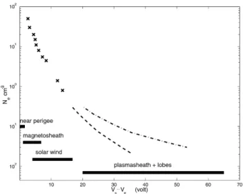
A calibration of spacecraft potential measurements on Cluster has been done by data from the active plasma sounder Whisper (Fig. 2). So far, the calibration has only been car-ried out forVS−VP up to+15 volts, corresponding to plasma densities of the order of 0.8 cm−3. Values ofV
S −VP up
to+60 volts have been measured over the polar caps and the lobes. For these values ofVS −VP, the plasma
den-sity is of the order of 10−3cm−3and its determination will depend more on the electron energy than for smaller values ofVS −VP observed in the plasma sphere, magnetosheath
and the solar wind. Later comparisons with calibrated par-ticle experiments will make it possible to relateVS−VP to
Space-craft potential observations are used in several of the studies that follow.
4 Examples of high coherence wave events along the
Cluster orbit
4.1 Examples from spin-fit data
The four spacecraft Cluster mission provides the first oppor-tunity to determine the 3D, time-dependent plasma charac-teristics. The present nominal inter-spacecraft separation is 600 km in regions with the tetrahedron configuration, which determines the scales for study with the four spacecraft. A major consideration for wave observations in a fast-flowing medium is the Doppler effect. Waveform data from the four spacecraft in a tetrahedral configuration allow for the correc-tion of this effect when the wavelength is comparable with the inter-spacecraft separation. If the wavelength is small in comparison to this distance, then the determination of the wave normal directions on the four spacecraft yield informa-tion about the source locainforma-tion.
By looking at the electric field data from the four satel-lites over time periods of a few hours, it is easy to find struc-tures that look similar from all four instruments not only near large-scale boundaries. Cross-correlation of spin averaged (4 s) electric field data over 3 h intervals may be as high as 0.95 between all four satellites. To obtain more detailed in-formation on the coherency between spacecraft waveforms with periods longer than about 50 s, electric field events are selected from regions of 6−16REduring the days between 19 and 23 January 2001. The orbit during this period had an apogee at about 14:30 LT.
There are four main frequency ranges available for electric field observations by EFW: the continuous spin-fit averaged data (4 s), normal mode data sampled at 25 samples/s, burst mode data sampled at 450 samples/s and internal burst mode data with sampling rates up to 36 000 samples/s over short periods of time. Very often, high coherence between mea-surements in all these sampling ranges can be found between all four spacecraft.
Assuming that Cluster instruments observe plain waves of the form exp (kr−ωt,) one can see that the phase difference observed by each pair of satellites is1ϕ =k1r, where1r
is the inter-spacecraft vector separation. From the observed phase shift, one can determine thekvector of the wave and
the phase velocity. This information is then used to find the Doppler shift correction for the wave frequency1ϕ=kv.
Events are selected in regions with large fluctuations in the electric field. The events are shown here to demonstrate the fact that on time scales of 50 s or longer, signatures with very high correlation between observations on the four spacecraft are found in many regions of the Cluster orbit. In Fig. 3, the
Y-component (approximately in the GSEY direction) of the electric field for 8 events is shown. TheX-component was not included here, but shows very much the same behaviour (see also Fig. 1 for an overview of 23 January).
Fig. 2. Calibration of the spacecraft to-probe-potential difference (VS−VP) in solar wind with electron densities measured by
Whis-per(crosses). Dotted lines indicate the expected range of (VS−VP)
in the plasmasheath and lobes, to be calibrated later with particle experiments.
Most of the events show periodic waveform structures with one or more dominant peaks in the frequency range from less than 1 to 15 mHz, as shown in Table 1. During two of the events, 19 January, 07:10–07:44 UT and 23 January, 17:10–22:54 UT, there is a rather abrupt change from one fre-quency to a higher one, with the coherency equally high in both frequency ranges. Examples of two solitary structures are also included. A single pulse was observed on 23 January at 10:50 UT and a bipolar event was observed 23 January at 13:00. The pulse in the event on 23 January, 10:42–11:03 UT is a signature of compression. A solar wind shock was ob-served on ACE at approximately 10:00 UT with the param-eters of densityN = 10 cm−3, velocityv =550 km/s and magnetic field atB = 12 nT. Cluster was in the magneto-sphere inside the magnetopause before compression and was brought into the magnetosheath.
These wave events were chosen to illustrate that high co-herence electric field events between Cluster spacecraft oc-cur in many regions along the orbit and for many different waveforms. Further studies will be made to obtain the de-tailed characteristics and sources of these wave phenomena, by including data from other instruments on Cluster and data from possible ground-based effects.
Fig. 3.Time series plots from 8 events based on spin-averagedY-component electric field data. The overlay data from up to four spacecraft show good coherence over distances of several hundred km. Note that the time is given in hours and decimal of hours.
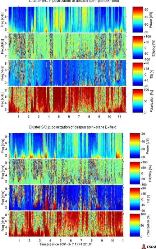
polarization concurrently from two of the Cluster spacecraft. The data was recorded when Cluster was in the solar wind and shows some distinct localized patches of electrical activ-ity. There is no obvious correlation in the activity between the spacecraft measurements, indicating a spatial extent of less than the spacecraft separation.
The polarization parameters are defined according to
I =D |EX|2+ |EY|2/2E (1)
v=(pV )/(2I ) (2)
φ=arctan(U/Q)/2 (3)
Table 1.Wave event characteristics
Event Location SC 1 Region Spectrum Phase
19 Jan 00:24 UT, 6.10RE Auroral oval or Single peak at Approx. const.
00:00–00:43 UT [−2.59, 0.66, 5.48]GSE Plasmasphere 2 mHz but irregular
19 Jan 04:24 UT, 10.46RE Plasmasheath/lobe 4 Peaks at 1, 0.05 Hz for
04:01–04:52 UT [1.17, 5.63, 8.74]GSE boundary 2, 5, 8 mHz 0–180◦
19 Jan 07:30 UT, 13.14RE Magnetosphere 2 Peaks at 10, 0.04 Hz for
07:10–07:44 UT [4.06, 8.37, 9.28]GSE lobe/plasmasheath 1.5 mHz 0–180◦
19 Jan 13:08 UT, 16.65RE Solar wind/ Peak at Approx. const.
13:03–13:14 UT [8.47, 11.61, 8.41]GSE magnetosheath 15 mHz but irregular
19 Jan 13:34 UT, 16.85RE Solar wind Peak at 2 mHz 0.09 Hz for
13:28–13:45 UT [8.76, 11.78, 8.28]GSE 0–1806◦
23 Jan 10:50 UT, 8.71RE Magnetosphere/ A single Const phase
10:42–11:03 UT [5.18, 0.32,−6.99]GSE magnetosheath structure to 0.06 Hz
23 Jan 13:00 UT, 6.01RE Near Southern Bidirectional
12:51–13:12 UT [1.74,−1.61,−5.78]GSE auroral oval structure
23 Jan 20:00 UT, 7.74RE North auroral oval 90 min period 0.09 Hz for
17:10–22:54 UT [−1.15, 2.73, 7.15]GSE to magnetosheath and 0.8 mHz 0–180◦
Q=D|EX|2− |EY|2 E
(5)
U=2DRE EXEY ∗ E
(6)
V =2DI m EXEY ∗ E
(7) andEX, EY are electric field components in GSM
coordi-nates and the bracketshidenote time averaging (we assume a time dependence of∝exp(+iωt). The four parameters of the electric field in the spin plane areI the power,v the de-gree of ellipticity,φthe tilt angle, andpthe degree of polar-ization. The sign ofvis such that positive values correspond to a positive sense of rotation of the electric field along the
Z-axis. The tilt angle is relative to the positiveX-axis. They are related to the Stokes parameters but do not necessarily refer to the transverse electric field components of an elec-tromagnetic wave.
A remarkable feature of the polarization spectra of this electrical activity is that for any given time and spacecraft, the polarization is virtually identical over the entire fre-quency band of the EFW burst mode. By comparison, at times when low electric power is observed, no particular po-larization is favored as expected, indicating good instrumen-tal conditions for such polarization measurements. Further-more, the ellipticity shows that the electric field is consis-tently linearly polarized to within a few percent with no ex-ceptions.
5 EFW observations in the plasmasphere
Near the perigee passes, the Cluster spacecraft have quick en-counters with the inner magnetosphere down toL=4, dur-ing which the satellites often skim the plasmapause region.
This boundary usually appears as a steep density decline, typically at aboutL = 3−6, but for disturbed conditions it may move withinL=3, whereas for very quiet conditions it can expand toL=12 (Laakso and Jarva, 2001).
Under magnetically quiet conditions (approximately
Kp < 3), the Cluster satellites usually cross the plasma-pause and enter the plasmasphere. This region, consisting of thermal plasma escaping from the ionosphere, appears as a dense torus around the Earth, where the charged particles rotate around the Earth at the same angular velocity as the Earth. This corotation of the plasmasphere is accompanied by an earthward pointing corotation electric field that forms closed equipotentials encircling the Earth (Volland, 1984). In fact, in a quasi-static model, the plasmapause can be de-fined as the last closed equipotential in a steady-state mag-netosphere with a constant convection field (Lemaire and Gringauz, 1998).
For increasing magnetic activity, magnetospheric convec-tion is enhanced and the locaconvec-tion of the flow separatrix moves rapidly earthward. In such conditions, the outer plasmas-phere becomes strongly structured, and plasmaspheric mate-rial will appear beyond the plasmapause. Such dense plasma elements become detached from the plasmasphere and drift away under the influence of the magnetospheric convection (Carpenter and Lemaire, 1997).
Fig. 4.Polarization plots of internal memory burst data. The panels of polarization are from top to bottom, respectively, the total powerI, the degree of ellipticityv, the tilt angleφ, and the degree of polarizationp.
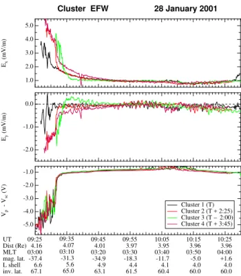
crossing, soon after 10:30 UT. The panels from top to bottom are the electric fieldEXandEY components in the magnetic
field line coordinate system and the potential difference be-tween a biased probe and the spacecraft; the field line coor-dinates are defined so that theZcoordinate is along the mag-netic fieldB, theXcoordinate is in the plane of the magnetic
field line and perpendicular toZ, pointing generally towards the equator, and theYcoordinate completes the frame of ref-erence and points generally westward.
plasma-pause is known to experience large changes in its geocentric distance (Laakso and Jarva, 2001). The density profiles may look quite similar, but a closer examination of the observa-tions reveals plenty of discrepancies in the region just out-side the plasmapause. Such irregularities are quite common for disturbed intervals, and this example was taken during moderate geomagnetic disturbances, as indicated by the pre-liminary AE index (data not shown here).
TheEXcomponent is responsible for the corotation flow,
and at this altitude, the corotation electric field (Ecor) is
ex-pected to be 0.9–1.0 mV/m and its value varies with distance (r) asr2; the corresponding drift velocity is about 2 km/s eastward. The top panel shows that outside the plasma-pause, the convection electric fieldEconis significantly larger than Ecor, and the convection direction is primarily
east-ward, as expected in this local time sector. TheEY
com-ponent, displayed in the middle panel, yields roughly the ra-dial drift velocity so that a negative value indicates an out-ward drift velocity. It vanishes in the plasmasphere, but from the outer plasmaspheric regions into the convecting magne-tosphere, it becomes increasingly important. The differences between the electric field measurements on the four satellites are quite remarkable, which only tells us that the outer plas-masphere is dynamically a very interesting plasma region, which deserves more multi-point measurement intervals with the Cluster satellites.
6 Large-amplitude auroral electric fields observed by
Cluster near perigee
Large-amplitude electric fields represent a common feature on auroral field lines at altitudes above a few thousand kilo-meters, as shown by a number of spacecraft such as Dynam-ics Explorer 1, Viking, Polar and FAST and in the return cur-rent region at altitudes as low as 800 km, as was first shown by Freja (Marklund et al., 1997). In many studies, such ob-servations have been interpreted in terms of quasi-static field-aligned electric fields (directed upward and downward in the upward and downward current regions, respectively) located below or partly below the spacecraft. In a recent study, large-amplitude electric fields observed by Polar were interpreted as signatures of Alfv´en waves carrying enough Poynting flux to produce intense auroral arcs (Wygant et al., 2000).
The objective of the present study is to investigate the elec-tric field on and adjacent to auroral field lines using data ob-tained near perigee, where the four Cluster spacecraft are aligned roughly as pearls on a string. With a time separa-tion of a few minutes between the Cluster spacecraft passing across the auroral field lines, the spatial and temporal char-acteristics of the electric fields can be investigated in much greater detail than from the single satellite observations re-ported in the past. The long-term objective of this study is to gain insight about the energy transport between the magne-tosphere and the auroral ionosphere, whether it may be de-scribed by a quasi-static current circuit or by an Alfv´en wave scenario. This is a fundamental question which, however,
Cluster EFW 28 January 2001
5.0 4.0 3.0 2.0 1.0 Ex (mV/m)
09:25 09:35 09:45 09:55 10:05 10:15 10:25 Time (UT) -2.0 -1.0 0.0 Ey (mV/m)
09:25 09:35 09:45 09:55 10:05 10:15 10:25 Time (UT) -5.0 -4.0 -3.0 -2.0 -1.0 Vp - V sc (V)
Cluster 1 (T) Cluster 2 (T + 2:25) Cluster 3 (T – 2:00) Cluster 4 (T + 3:45)
09:25 4.16 03:00 -37.4 6.6 67.1 09:35 4.07 03:10 -31.3 5.6 65.0 09:45 4.01 03:20 -34.9 4.9 63.1 09:55 3.97 03:30 -18.3 4.4 61.5 10:05 3.95 03:40 -11.7 4.1 60.4 10:15 3.96 03:50 -5.0 4.0 60.0 10:25 3.96 04:00 +1.6 4.0 60.0 UT Dist (Re) MLT mag. lat. L shell inv. lat.
Fig. 5.Observations by the EFW experiment in the inner magneto-sphere on 28 January 2001, 09:25–10:30 UT. The two electric field components in the field line coordinate system and the differential potential measurements are shown. The plasmapause is crossed by Cluster1 at ∼09:32 UT and by the other three spacecraft within ±4 min of that time, as shown by the legend in the bottom panel.
requires the detailed analysis of magnetic field and particle data, in addition to the electric field data. This analysis is outside the scope of this initial study.
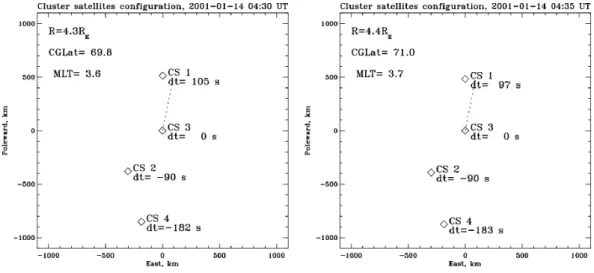
Fig. 6.Relative positions of the four Cluster spacecraft in a plane perpendicular toBat 04:30 and 04:35 UT on 14 January 2001. Vertical and horizontal axes represent distances in the geomagnetic poleward and eastward directions. Spacecraft 3 is located at the center. The time differences (dt) between the four spacecraft to that of spacecraft 3 are indicated at the spacecraft positions. The geocentric distance, corrected geomagnetic latitude and magnetic local time for spacecraft 3 are given at the top, left. The dotted line indicates the direction of the velocity component perpendicular toBfor spacecraft 3.
of roughly 40–50 km. In the upper four panels of Fig. 7, one can see the sunward component of the electric field in the spin plane versus time after 04:27 UT for each of the four spacecraft, followed by four plots of the duskward electric field component and four plots of the negative of the satellite potential as derived from the EFW data (for a description of the EFW instrument, see above).
To be able to directly compare the data between the four spacecraft, the time lines for satellite 1, 2, and 4 have been shifted relative to the reference time line for satellite 3 by the numbers given in Fig. 6. Note that the entry and the exit out from the region which is characterized by the pres-ence of small-scale irregular electric field variations and a de-crease in the satellite potential (dede-crease in plasma density), is roughly the same for spacecraft 2, 3, and 4 and somewhat displaced for spacecraft 1. This might be explained by an equatorward motion of the auroral oval during the time span between the oval entries by spacecraft 1 and spacecraft 3. The time between the entry and the exit of the region which is characterized by irregular electric fields and decreases in the satellite potential is roughly the same for all spacecraft, around 700 s, which corresponds to a 350 km distance in the ionosphere or a latitudinal width of 3.2◦. Polar UVI im-ager data from this time and the local time sector (not shown here) around 03:30 MLT indicate an oval width of 5–6◦and that the equatorward edge of the oval is located at 69.5◦. This is in good agreement with the location of the Cluster space-craft at the entry into the region of irregular fields. Thus, the irregular electric fields seem to dominate within the central and equatorward portions of the oval, i.e. primarily within the large-scale region 2 upward field-aligned currents. Note that the sunward electric field component is much weaker on spacecraft 4 than on spacecraft 1–3. The same is true for the satellite potential which is much weaker (larger electron
density) and flatter on spacecraft 4 than on spacecraft 1–3. What persistent or repetitive features observed by two or more spacecraft can we distinguish from these electric fields and satellite potential traces? Moving from left to right, the entry into the oval is characterized by the onset of electric field fluctuations and a slow decrease in the negative of the satellite potential. Next, a region of very bursty electric fields reaching magnitudes exceeding 100 mV/m on spacecraft 4 (duskward component) are observed by spacecraft 3 almost simultaneously at aroundT =260 s (marked with a vertical line A in Fig. 7) and about 10 s and 25 s later on space-craft 2 and spacespace-craft 1, respectively. The most pronounced and persistent feature is the intense converging electric field structure seen by spacecraft 1, 2, and 3 at aroundT =375 s (marked with line B in the figure). It is colocated with a steep gradient in the satellite potential, and thus, a gradient in the plasma density (most pronounced on spacecraft 3). The fact that the field is convergent indicates that the structure is re-lated to an upward field-aligned current, presumably associ-ated with an arc. The peak electric field reaches 90 mV/m on spacecraft 2 and 3 and 55 mV/m on spacecraft 1. The width of the structure ranges between 10 and 15 km mapped to the ionosphere, which is consistent with the characteristic scale size of discrete auroral arcs. Finally, between 730 and 780 s (marked with the vertical lines C and D, respectively, in Fig. 7) on spacecraft 2, 3 and 4 and about 25 s later on space-craft 1, a small positive duskward electric field is observed, i.e. the electric field has the same direction as that which is typical of the polar cap. This duskward electric field interval was preceded by a region of irregular electric fields.
In summary, the characteristics of the auroral electric field at an altitude of about 3.3RE have been examined based
Figure 7
A B C D
Fig. 7.Electric field and satellite potential data from near-perigee auroral field line crossings by the four Cluster spacecraft on 14 January 2001. The time axis is seconds relative to 04:27 UT on spacecraft 3, while the time axes for the other spacecraft have been shifted. The vertical lines A–D at 260, 375, 730 and 780 s, respectively, are included to facilitate the location of regions described in the text.
aligned roughly as pearls on a string. The geophysical data available indicate that the crossing took place during the re-covery phase of an auroral substorm peaking in activity about half an hour prior to the crossing. Although there are dif-ferences seen particularly in the electric field fine structure, common large-scale features are seen both in the electric field and in the satellite potential that persist during the time span of 287 s between the crossings of spacecraft 1 and spacecraft 4. The entry and the exit of the region characterized by
re-Fig. 8. An example of a magnetopause crossing (between 10:15– 10:25 UT) where the spacecraft entered the magnetosheath and re-turned three minutes later. The figure demonstrates the detailed be-haviour of the spacecraft potential (plasma density), electric field and plasma flow near the boundary.
gion of bursty electric fields reaching above 100 mV/m on spacecraft 4 located about 50 km equatorward of the conver-gent electric field structure. Moreover, a region of irregular electric fields followed by an increase in the duskward elec-tric field component was observed near the poleward edge of the oval where the electric field was changing to that which is characteristic of the polar cap.
The most pronounced feature was a convergent electric field structure seen by spacecraft 1–3, but most pronounced on spacecraft 2 and 3 with peak values of 90 mV/m which, if mapped to the ionosphere, would amount to almost 1 V/m. The structure, with a width of 10–15 km mapped to the iono-sphere, was colocated with a steep gradient in the plasma density and presumably associated with the upward field-aligned current of a discrete arc within region 2. The fact that this structure retained its major features for more than three minutes strongly suggests that it represents the upward
solar wind at approximately 07:00 LT. The solar wind speed was 320 km/s and the plasma density 5 cm−3. The magnetic
fieldBZcomponent varied from north to south with a
mag-nitude of 3–4 nT.
Some of the passages of Cluster into the magnetosheath showed a positiveBZand others have a negative value. The
latter case is chosen as an example in Fig. 8. The upper panel demonstrates that the density increased to magnetsheath val-ues at 10:17:40, about 10 s beforeBZ started to turn
south-ward. The most interesting part is thatEY is positive in the
current layer which can be estimated to be in the−XandY
direction. The current layer, as seen in the magnetic measure-ments (not shown here), was at about 10:17:50 to 10:18:10 for the magnetopause inward motion, and at 10:20:35 to 10:20:55 for the outward motion. This indicates thatE•I
is positive and that electromagnetic energy is transformed to kinetic energy, a signature of reconnection.
The outward motion of the magnetopause does not have the same electric field signature and it is difficult to estimate
E•I. The density drops in the current layer and there appears to be no dense plasma inside the current layer in this case.
This example is meant to illustrate the tremendous possi-bilities of studying the magnetopause with complete analy-sis of magnetic and electric fields, and particles on all four spacecraft.
7.2 Multipoint observations of waves in the lower hybrid frequency range near the magnetopause
amplitude V -30 -25 -20 -15 -10 -5
Start: 2001-01-14 15:02:00.0 minutes
2.0 3.0 4.0 5.0 6.0 7.0
Interval: 328.0s q0 [-32,-4 V]
q1 [-32,-4 V] q2 [-32,-4 V]
q3 [-32,-4 V]
fft(q4)
Start: 2001-01-14 15:02:00.0 Interval: 328.0s minutes
2.0 3.0 4.0 5.0 6.0 7.0
frequency[Hz] 0 2 4 6 8 10 power [(mV/m)^2/Hz] 1 0.1 0.01 0.001 0.0001 1E-05 1E-06 fft(q8)
Start: 2001-01-14 15:02:00.0 Interval: 328.0s minutes
2.0 3.0 4.0 5.0 6.0 7.0
frequency[Hz] 0 2 4 6 8 10 power [(mV/m)^2/Hz] 1 0.1 0.01 0.001 0.0001 1E-05 1E-06 fft(q12)
Start: 2001-01-14 15:02:00.0 Interval: 328.0s minutes
2.0 3.0 4.0 5.0 6.0 7.0
frequency[Hz] 0 2 4 6 8
10 power [(mV/m)^2/Hz] 1
0.1 0.01 0.001 0.0001 1E-05 1E-06 fft(q16)
Start: 2001-01-14 15:02:00.0 Interval: 328.0s minutes
2.0 3.0 4.0 5.0 6.0 7.0
frequency[Hz] 0 2 4 6 8
10 power [(mV/m)^2/Hz] 1
0.1 0.01 0.001 0.0001 1E-05 1E-06 fft(q20)
Start: 2001-01-14 15:02:00.0 Interval: 328.0s minutes
2.0 3.0 4.0 5.0 6.0 7.0
frequency[Hz] 0 2 4 6 8 10 power [(nT)^2/Hz] 1 0.1 0.01 0.001 0.0001 1E-05 1E-06 1E-07 1E-08 1E-09
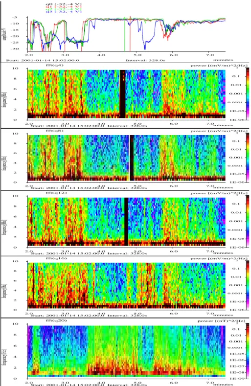
Fig. 9.Data from the four Cluster spacecraft near the dusk magnetopause. The top panel is the negative of the spacecraft potential, panels 2–5 are the electric field data from spacecraft 1–4 and the bottom panel is the magnetic field data obtained by STAFF.
for some time. Satellite 4 leaves the magnetosheath for about half a minute after 15:05:00. Panels 2–5 show EFW electric field data from satellites 1 to 4 at frequencies up to 10 Hz. It is clear that broadband (in the satellite frame) waves are seen on all spacecraft at the density gradients and in the lower density magnetosphere and boundary layer regions. (The signal up to around 1 Hz in this figure is partly due to the quasi-static electric field) In particular, note the waves
Fig. 10. Electric field component and spacecraft potential at a se-quence of magnetopause crossings. Strong electric field turbulence is co-located with the boundary crossings (density gradients).
in the magnetosheath.
In these regions, the proton gyrofrequency and the lower hybrid frequency are about 0.3 and 10 Hz, respectively. Cur-rents at the magnetopause, density gradients, and shear in the quasi-static electric field (Sibeck et al., 1999, and references therein) can cause waves in this frequency range. An impor-tant question is how much of the broadband emissions in the satellite frame is due to true time variations, and how much is caused by a Doppler shift due to the moving magnetopause. Detailed studies (see Andr´e et al., 2001, this issue) indicate that in the magnetopause frame, both are essentially static, and also time varying. In addition, electric field structures can be present. Future investigations will include estimates of the wave polarization using single satellites, and tests of the coherence of signals between satellites, to study the gen-eration, the frequency in the frame of the moving topause, and the importance for transport across the magne-topause of these waves.
7.3 Kinetic Alfv´en and drift waves at the magnetopause Low-frequency turbulence extending from well below the ion gyrofrequencyfci up to the lower hybrid frequencyflh
is of considerable interest for space plasmas since it con-tains a large wave power, but its nature and origin is not well understood. The ELF turbulence is observed by the satellites in all active regions of the magnetosphere, and in particular, at the magnetopause layer, where it is expected to play an important role in the processes of reconnection, diffusion, mass and energy transport. Earlier studies of broadband turbulence measured in the auroral zone by Freja (Stasiewicz et al., 2000) and in the high-latitude boundary layer by Polar (Stasiewicz et al., 2001) indicate that this turbulence consists of short spatial scale dispersive Alfv´en waves, which are Doppler shifted in the satellite frame by plasma motion with respect to the satellite. Similar analy-sis has been carried out on Cluster data for an event from multiple boundary crossings. During a single passage on 31
Fig. 11.Electric field power at time 10:26 UT.
December 2000, 120 magnetopause crossings were recorded during several hours, from 09:00–16:00 UT. These magne-topause crossings are characterized by strong density gra-dients where the density increases from a magnetospheric value of 0.1 cm−3to about 10 cm−3in the magnetosheath over a distance of 500–1000 km. An example is shown in Fig. 10. The curve (scp) with the potential shows that the spacecraft was in a region with high density plasma (mag-netosheath) when an outward boundary motion moved the satellite into the magnetosphere and then back toward the magnetosheath at 10:29 UT. The structure at 10:26 UT corre-sponds to a partial inward/outward boundary motion. Using data from the four spacecraft we can estimate the boundary speed to be 170 km/s and the thickness of the density ramp to be 1000 km for the first crossing. The electric field in Fig. 10 exhibits strong turbulence during the boundary cross-ings. Turbulent fields of 5 mV/m are larger than the DC field of 2 mV/m, and are clearly co-located within the density gra-dients. The power spectrum of the electric field measured around 10:26 UT is shown in Fig. 11. The electric field spec-trum shows a power-law dependence.
Fig. 12. Spacecraft potential and electric field data. Top panel shows the negative of the satellite potential. The middle panel shows the radial component of the electric field which has been lowpass filtered at 0.1 Hz. There is a data gap around 15:05 UT. The bottom panel shows the spectrogram of the non-filtered electric field.
shifted dispersive Alfv´en waves at small perpendicular wave-lengths. Further studies are needed to assess the generation mechanism of these waves and structures, and their role in the process of energy/mass transport and diffusion across the magnetosphere.
7.4 Example of magnetopause surface wave with a period of several tens of seconds
Here we show an example where Cluster satellites observe multiple magnetopause crossings with periods of several tens of seconds (Pc3 time scale). The magnetopause crossings were at 14:50–15:20 UT, on 14 January 2001 in the early afternoon sector (∼15 MLT). Using data from all 4 space-craft we show that multiple crossings are caused by an anti-sunward propagating surface wave. We estimate the char-acteristic spatial scales of the wave and the magnetopause itself. In terms of the magnetopause, here we mean the re-gion where the plasma changes its character from magneto-spheric to magnetosheath-like, which is seen as a jump in the satellite potential. This does not necessarily agree with a magnetopause current region.
Figure 12 shows an overview of the magnetopause cross-ing as seen by one spacecraft. The top panel shows the nega-tive of the spacecraft potential; we can distinguish regions of magnetospheric plasma (large negative values) and magne-tosheath plasma (small negative values). The sharp transition between the two indicates that the magnetospheric plasma is most likely on the closed field lines. Data from ion and elec-tron instruments confirm this (not shown). The middle panel shows the radial component of the electric field (positive is outwards). We can see that the lowest electric field values are within the magnetosphere, but not in the direct
neighbour-Fig. 13.For all four spacecraft, potential and the radial component of electric field, lowpass filtered at 0.06 Hz.
hood of the magnetopause (jump in the spacecraft potential). However, near the magnetopause crossing, we see large neg-ative values of the electric field inside the magnetosphere. The correspondingE×Bvelocity is of the order of 200 km/s
anti-sunward that is comparable to the plasma velocity in the magnetosheath. Similar electric fields has been seen by Geo-tail (Mozer et al., 1994). The bottom panel shows the electric field spectrogram where we can see increased wave activ-ity at the magnetopause in the frequency range both above and below the proton gyrofrequency (it is between 0.2 and 0.4 Hz). From the top panel of Fig. 12 around 15:03 UT, we can identify four magnetopause crossings with a period of about 30–40 s. The same crossings can be identified as os-cillations in the electric field. However, the electric field data show several additional oscillations of the same period be-fore crossings can be seen in the satellite potential, i.e. during this period the electric field can be used as the remote sensor of the magnetopause disturbances. We will study closer the magnetopause crossings that are clearly seen in the satellite potential.
Fig. 14. Top panel shows the satellite potential of all four spacecraft for an outbound magnetopause crossing at 15:02:10 UT, 14 January 2001. During this day, the EDI instrument on spacecraft 2 significantly affected the spacecraft potential in low density plasma (−V scbelow about−20V). The middle panel shows the potential structure as a function of distance. The velocity has been obtained from the time when the spacecraft potentials cross−15V value. The obtained velocity in GSE coordinates isv =(−103,14,26)km/s. The bottom panel is a combined plot:X-axis is in the direction antiparallel to the velocity of the magnetopause,Y-axis is perpendicular toXand the magnetic field (thus in the plane of the magnetopause).The satellite trajectory is projected onto this plane and colored according to−V scvalues. In addition, the black lines show the direction of the electric field.
plasma sheet ion with a characteristic energy of 4 keV. To proceed with phase velocity estimates, we have to look in more detail at separate magnetopause crossings. In Fig. 14, we zoom into one outbound magnetopause cross-ing at about 15:02:10 UT. The top panel shows that most of the change in the satellite potential occurs within a time pe-riod of less than a second. The spatial scale is shown in the middle panel. It is obtained by estimating the velocity of the magnetopause along its normal direction, which in this case, is 107 km/s, from the times at which −V sc at all 4 spacecraft pass the 15V level. The assumption is made that the magnetopause on the scale of satellite separation is flat and moves with a constant velocity. We can see that most of the satellite potential change is within a distance of less than 100 km. This is comparable to the gyroradius of 100 eV magnetosheath protons, which is about 70 km. In the bot-tom panel, we show the electric field data around the mag-netopause crossing in the reference frame moving with the magnetopause (withoutV×Bcorrection). The electric field
has been calculated assuming that its component parallel toB
is zero. One can see the large electric fields inside the magne-tosphere which have both tangential and normal components with respect to the magnetopause. During this crossing, the field becomes small approximately 100 km before the
mag-netopause; however, during other crossings, the field can be large until the magnetopause itself is reached. At the magne-topause itself, the field is strong but very variable.
From the difference in magnetopause velocity directions for the inbound and outbound crossings we can see that the multiple crossings, are consistent with surface waves that propagate anti-sunward along the magnetopause. Therefore, we would like to observe the wave structure in the refer-ence frame that moves with the phase velocity of this face wave. We estimate the direction and size of the sur-face wave phase velocity such that it is in the plane defined by the inbound and outbound crossings and is consistent with both of them. Here, for simplicity, we take only two crossings (at 715 s and 730 s). The obtained phase veloc-ity is about 190 km/s anti-sunward along the magnetopause,
v =(−144,79,89)km/s in GSE, and is comparable to the magnetosheath plasma velocity. We can compare the angles between this phase velocity and the magnetopause normals at the outbound (55◦) and inbound (69◦) crossings. We see that the outbound crossing is slightly steeper.
In Fig. 15, we plot a combined plot, in the same way as in the bottom panel of Fig. 14, to show the electric field and potential in the frame of reference of the surface wave (E
Fig. 15.A combined plot: X-axis is in the direction antiparallel to the phase velocity,v=(−144,79,89)km/s GSE, of the surface wave along the magnetopause,Y-axis is perpendicular toXand the magnetic field (thus in the plane of the magnetopause). The satellite trajectory is projected onto this plane and colored according to−V scvalues. In addition, the black lines show the direction of the electric field.
Spacecraft 1, 2 and 3 project close to each other since the plane defined by them is close to being parallel with the mag-netopause plane. One should note the different scaling on the axis. The wavelength of the surface wave along the magne-topause is of the order of 6000 km. In the regions of the magnetopause crossings the electric field inside the magne-tosphere is almost perpendicular to the phase velocity of the surface wave without large variations in the electric field di-rection. Thus, the electric field does not follow large varia-tions in the normal direction of local magnetopause crossings (as we see from above, this variation can be more than 60◦) but tends to agree with the normal direction of the “mean” (undisturbed) magnetopause.
Further studies of this and similar magnetopause crossings should address the questions of whether these surface waves with periods of several tens of seconds are driven by the so-lar wind or generated through KelvHelmholtz type of in-stabilities. What is the source of the large electric field just inside the magnetopause and does it map to the ionosphere? Does this electric field contribute to the convection potential drop?
7.5 Solar wind and magnetosheath flows
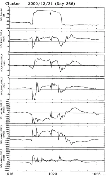
An example is given of a period of more than three hours, during which the Cluster spacecraft were in the magne-tosheath and solar wind (Fig. 16). The data from all four spacecraft are similar for this time interval. For simplicity, only the data from spacecraft 4 is illustrated. During the plotted time interval, the ACE spacecraft was in the upstream solar wind, where it measured an average plasma density of about 6 particles/cm3and a flow speed of 310 km/s. At about 19:35 UT, ACE observed an abrupt northward turning of the interplanetary magnetic field, which arrived at Cluster near 21:00 UT to modify the fields as discussed below.
The top graph is the spacecraft potential, which is a func-tion of plasma density. It shows that spacecraft 4 was in the magnetosheath between about 19:49:30–20:03:30 UT and again between about 21:45:30–22:40:00 UT. During the
re-mainder of the figure, spacecraft 4 was in the solar wind, where the average spacecraft potential of about 7 volts cor-responds to an average density of about 7 particles/cm3 (which compares to the average ACE density of about 6 par-ticles/cm3).
The second and third panels give the spin period averaged electric field components in the GSE X- andY-directions. The field was turbulent in the magnetosheath and relatively quiet in the solar wind. The central feature of this electric field data is thatEXandEY were correlated, as they
gener-ally are in the solar wind and magnetosheath. This correla-tion can be understood by assuming that the total flow veloc-ity in the GSE-Zdirection, VTOTZ, is 0 (as it generally is in
the magnetosheath and solar wind). Then,
V T OTZ=0=vk(BZ/B)+(EXBY −EYBX)/B2 (8)
This equation may be viewed as giving the parallel flow, vk, as a function of the field quantities. Substituting this func-tion into expressions for VTOTX and VTOTY gives, after
setting the parallel electric field to zero,
V T OTX=EY/BZ (9)
V T OTY = −EX/BZ (10)
These two equations show thatEX,EY, andBZcorrelate
with each other. Thus, the correlation of the electric field components is a consequence of the total flow being approx-imately constant and confined to the ecliptic plane. A further consequence of this correlation is that the total flow (not just theE×Bcomponent of the flow) is obtained from the
ra-tios of field quantities given in Eqs. (9) and (10) and that are plotted in the lowest two panels of Fig. 16.
Several conclusions may be reached from the lowest two plots:
Fig. 16.Example of flow velocities for a period of more than three hours, during which the Cluster spacecraft were in the magnetosheath and solar wind.
2. In the magnetosheath, theX-component of the flow is reduced by a factor of about 4 relative to that in the so-lar wind. The magnetosheath flow appears much less turbulent than the fields from which it was obtained. 3. In the solar wind, near 21:00, the electric fields changed
sign but the solar wind flow velocity did not. This is proof that the calibration offsets in the field measure-ments are correct.
4. The averageY-component of the flow in the solar wind was about+60 km/s, which is consistent with the ex-pectations associated with the aberration angle of the solar wind flow.
This study shows that the electric field, its offsets, and the spacecraft potential have been calibrated to an absolute accu-racy of better than 10% in this and several similar examples.
TheZ-component of the magnetic field has been similarly calibrated.
8 Turbulent boundary layer
Figure 17.
Fig. 17. An outbound turbulent boundary layer crossing by Cluster on 2 February 2001. Panels (a) and (e) showEXbi-spectrogram and
integrated spectrum at 16:00–17:30 UT, respectively. Panel (b) displays a waveletEX spectrogram in the range of 3–20 mHz, inferred
cascades are depicted by black lines. Panel (c) demonstrates the electric fieldEX waveform and panel (d) the magnetic field. Note, in
particular, that the magnetic field drops to very low values in a few cases. Insert 1 in panel (d) shows the most characteristic example of the cascade-likeEY wavelet spectrogram at 16:10–16:25 UT (see text for details).
described in Savin et al. (2001) (see there also the respective references).
In Fig. 17, we depict an outbound TBL crossing of the Cluster spacecraft 1 at high latitudes. In panel (d), the mag-netic field|B|summary plot illustrates a very common TBL signature of “diamagnetic bubbles” with magnetic field drops down to a few nT. We have studied the spacecraft potential behaviour that reflects plasma density fluctuations induced by the “diamagnetic bubbles”. While having generally the same character as the electric field components, these fluc-tuations have no such characteristic peculiarities as the mag-netic field components described by Savin et al. (2001). We think this is due to the strong dominance of the transverse waves in the TBL while the density variations are connected with the compressible fluctuations.
In panel (c) of Fig. 17, we depict theEXwaveform in the
GSE frame. One can see that the general electric field activ-ity tends to correlate with the|B|gradients in the panel (d).
Panel (b) displays a wavelet colour-coded spectrogram ofEX
in the frequency band 0.3–20 mHz. Panels (a) and (e) rep-resent a wavelet bi-spectrogram and wavelet integrated spec-trum, respectively, in the bands 0.6–99 and 0.35–170 mHz (see the wavelet description below).
We start from the panel (b) description. Wavelet analysis is a powerful tool to investigate turbulent signals and short-lived structures. In order to examine the transient non-linear signal in the TBL, we have performed the wavelet transform with the Morlett wavelet:
W (a, t )=CX nf (ti)
to 200 mHz and then followed by intensive wave-trains at higher and higher frequencies. The lower intensity branch descends to a few mHz resembling a reverse cascade. An-other reverse cascade (instant) is depicted on the right part of Insert 1. In panel (b), we would like to outline the processes at about 0.4–2 and 5–9 mHz, where the maximums near the two lowest frequencies are visible throughout the TBL, i.e. the region of the “diamagnetic bubbles” in panel (d). Their junction and intensification seem to trigger a direct cascade. Both continuous and spiky (i.e. low and high frequency) ac-tivities in panel (b) correspond to maximums in the integrated spectrum in panel (e), (note that the latter was calculated for 16:00–17:30 UT). In the high frequency disturbances on panel (e) two characteristic slopes are seen: −1.027 at 0.006–0.08 Hz and−2.01 at 0.08–0.2 Hz. The slope at the higher frequency corresponds to the self-consistent plasma turbulence and is similar to the one observed in the magneto-tail. The lower frequency part may be related to the “flicker” noise and is also a general feature of non-linear systems near a state of self-organized criticality. The transient wave-trains, visible in panel (b) at 5–10 mHz should provide the mean for the energy transfer towards the higher frequencies, in con-trast to the chaotic quasi-homogeneous processes at higher frequencies. The electric field spectral slopes remarkably re-semble that of the magnetic spectra in the TBL from Polar and Interball-1 data (Savin et al., 2001).
We would like to do a further test for possible self-organization in the TBL processes. We use the wavelet-based bicoherence to check if the wave-trains at different frequen-cies really constitute the coherent interactive system with multi-scale features. In the SWAN software, for the wavelet analysis, the bicoherence is defined as:
b2 a1, a2= |B a1, a2|2/
n X
|W a1, ti W a2, ti|2
X
|W a, ti|2 o
(12) withB(a1, a2)representing the normalized squared wavelet
bi-spectrum:
B a1, a2=
X
W∗ a, tiW a1, tiW a2, ti (13)
theW (a, t )is the wavelet transform according to (11) and the sum is performed, satisfying the following rule:
1/a =1/a1+1/a2 (14)
order non-linearity in the system. We will not discuss here the weaker higher-order non-linear effects, which might also contribute to the TBL physics.
In panel (a) of Fig. 17, we present a bicoherence spectro-gram for GSE EX in the Cluster outbound TBL. The
fre-quency plane (f1,f2) is limited by the signal symmetry
con-siderations and by the frequency interval of the most charac-teristic TBL slope of∼1 in panel (e). As we mentioned in the previous paragraph, the bicoherence in the TBL displays the second and higher harmonic non-linear generations and, most likely, the 3-wave processes. We assume cascade-like signatures in Fig. 17 when the bicoherence at the sum fre-quency,f = f1+f2, has comparable a value with that of
point (f1,f2). In the case of the horizontal-spread maximum,
it implies that the wave at sum frequency interacts with the same wave at the initial frequency (say,fA) in the following 3-wave process:f3=fA+f, etc.; the initial wave spectrum
can be smooth, resulting in the continuous bi-spectral maxi-mum. One can see the most characteristic picture of the syn-chronized 3-wave processes in a rather wide frequency band in the horizontalspread maximum at ∼6-9 mHz in panel (a). It corresponds to a maximum and plateau on panel (e) and to the most intensive wave-trains in panel (b) at 16:10– 17:06 UT with the cascade-like features (see also Insert 1 and the discussion above). A maximum that is not continuous at ∼1–2 mHz (maximum at∼16:10–17:00 UT in panel (b)). A horizontal maximum is also present at∼0.6 mHz at the low-est frequency in panel (a) (while it is quite narrow in panel (a), we have checked that it is present on the lower frequency bi-spectrograms; see also panels (b) and (e)). A weak hor-izontal maximum in panel (a) at 3.5 mHz could correspond to a cascade-like event in panel (b) at∼17:13 UT. Numer-ous wave-trains in panel (b) at 15–19 mHz can contribute to the corresponding horizontal maximum in panel (a). Most of these maximums are also present in the spacecraft potential bi-spectrograms (not shown), with the most prominent ones are at 2–3 and 0.6 mHz.
mHz) fluctuations might resonate with the cusp flux tubes and provide a possible link to correlated solar wind interac-tions with the dayside magnetopause and cusp ionosphere.
We would like to emphasize that our consideration of the non-linear cascade scenario, while in agreement with the Interball-1 and Polar case studies, is a very likely hypothe-sis, which could be further checked using multi-spacecraft data at least for the lower frequencies. In addition, verifi-cation of wave vector sums conservation in 3(4)-wave non-linear processes, wave mode identifications, group velocity determinations, data transformations into de Hoffman-Teller or magnetopause frames, etc. are foreseen the verification of our hypothesis. For that study plasma moments and magnetic fields at the highest time resolution will be needed.
9 Summary
The coherence between observations of the electric field from the four Cluster spacecraft is very high, for frequen-cies below the spin period for several regions along the orbit. This preliminary study shows cross-correlation values of 0.9 or higher for the low frequencies, which indicates that true three-dimensional investigations can be carried out for many plasma phenomena. Wave spectra up to several kHz also show similarities that look encouraging for future detailed comparisons between spacecraft. It is also demonstrated that the spacecraft potential, a measure of the plasma density, is very useful for the identification and characterization of rapidly moving boundaries near the magnetopause, which is one of the primary regions for Cluster studies. The potential of four point-measurements are used, in particular, to evalu-ate surface waves with wavelengths of about 6000 km along the magnetopause. In the auroral oval region, the four satel-lite observations give important information on electric field structures. The preliminary study presented here indicates that the electric field structure on auroral field lines retained its major features for more than three minutes. This suggests that it represents the upward continuation of a quasi-static U-shaped potential contour associated with an auroral arc. The persistency of the structure provides support for a quasi-static auroral potential structure that extends at least to a geocentric distance of 4.3RE.
The large potential for three-dimensional investigations in several regions along the orbit is demonstrated and it may be expected that studies based not only on electric field data but also on observation from the full complement of instru-ments on board Cluster will open the way for great scientific discoveries.
Acknowledgements. Work on turbulent boundary layer was
par-tially supported by the grant INTAS 97-1612. We appreciate D. Lagoutte and his colleagues from LPCE/CNRS in Orleans for pro-viding the SWAN software used for the wavelet transform analysis. Magnetic field data from the FGM instrument (A. Balogh), electron density data from the Whisper instrument (P. D´ecr´eau) and search coil magnetic field data from the STAFF instrument (N. Cornilleau-Wehrlin) used in this study is greatly acknowledged.
Topical Editor M. Lester thanks H. Alleyne and P. Stauning for their help in evaluating this paper.
References
Andr´e, M., Behlke, R., Wahlund, J.-E., et al.: Multi-spacecraft ob-servations of broadband waves near the lower hybrid frequency at the Earthward edge of the magnetopause, Ann. Geophysicae, this issue, 2001.
Balogh, A., Dunlop, M.W., Cowley, W.H., et al.: The Cluster mag-netic field investigation, Space Sci. Rev., 79, 65–92, 1997. Carpenter, D. L. and Lemaire, J.: Erosion and recovery of the
plas-masphere in the plasmapause region, Space Sci. Rev., 80, 153– 179, 1997.
D´ecr´eau P. M. E., Fergeau,, P., Krasnosels’kikh, V., et al.: Early results from the WHISPER instrument on Cluster: an overview, Ann. Geophysicae, this issue, 2001.
Escoubet, C. P., Pedersen, A., Schmidt, R., and Lindqvist, P.-A.: Density in the magnetosphere inferred from the ISEE-1 space-craft potential, J. Geophys. Res., 102, 17, 595–609, 1997. Gurnett, D. A., Pickett, J. S., Huff, R. L., et al.: First results from
Cluster wide-band plasma wave investigation, Ann. Geophysi-cae, this issue, 2001.
Gustafsson, G., Bergstr¨om, R., Holback, B. et al.: The electric field and wave experiment for the Cluster mission, Space Sci. Rev., 79, 137–156, 1997.
Laakso, H. and Jarva, M.: Evolution of the plasmapause position, J. Atmos. Sol. Terr. Phys., in press, 2001.
Laakso, H., Pfaff, R., and Janhunen, P.: Polar Observations of Elec-tron Density Distribution in the Earth’s Magnetosphere, J. Geo-phys. Res., submitted, 2000.
Lemaire, J. F. and Gringauz, K. I.: The Earth’s Plasmasphere, Cam-bridge Univ. Press, CamCam-bridge, 1998.
Marklund, G., Karlsson, T., and Clemmons, J.: On low-altitude par-ticle acceleration and intense electric fields and their relationship to black aurora, J. Geophys. Res., 102, 17 509–17 522, 1997. Mozer, F. S., Hayakawa, H., Kokobun, S., Nakamura, M., Okada,
T., Yamamoto, T., and Tsuda, K.: The morningside low-latitude boundary layer as determined from electric and magnetic field measurements on Geotail, Geophys. Res. Lett., 21, 2983, 1994. Nakagawa, T., Ishii, T., Tsuruda, K., Hayakawa H., and Mukai, T.:
Net current density of photoelectrons emitted from the surface of the Geotail spacecraft, Earth Planets Space, 52, 283–292, 2000. Pedersen, A.: Solar wind and magnetosphere plasma diagnostics by
spacecraft electrostatic potential measurements, Ann. Geophysi-cae, 13, 118–121, 1995.
Pedersen, A., Mozer, F., and Gustafsson, G.: Electric field measure-ments in a tenuous plasma with spherical probes, AGU Geophys. Monograph 103, 1–12, 1998.
Pedersen, A., D´ecr´eau P. M. E., Escoubet, C.-P., et al.: Cluster four-point high time resolution information on electron densities, Ann. Geophysicae, this issue, 2001.
Savin, S. P., Borodkova, N. L., Budnik, E. Yu., et al.: Interball tail probe measurements in outer cusp and boundary layers, in Geospace Mass and Energy Flow: Results from the Interna-tional Solar-Terrestrial Physics Program, (Eds) Horwitz, J. L., Gallagher, D. L., and Peterson, W. K., Geophysical Monograph 104, AGU, Washington D.C., pp. 25–44, 1998.