DETERMINATION OF NEAR-OPTIMAL
MILD STEEL WELD BEAD GEOMETRY
USING THE CONTROLLED RANDOM
SEARCH METHOD
JOSEPH I. ACHEBO
Department of Production Engineering University of Benin, Benin City, Nigeria
MONDAY J. OMOREGIE
Department of Production Engineering University of Benin, Benin City, Nigeria
Abstract:
Weld quality is a very important determinant factor in assessing the integrity of any metallic manufactured product. Attempts in the past have been made to improve the quality of weldments through rigorous research has been known to be improved through the optimization of the welding process parameters. Several models have been used to optimize these process parameters by other researchers but in this study, the controlled random search (CRS) method was used. By using CRS method, the objective functions for the combinations of the sixteen experimental runs were calculated, the highest and lowest objective functions were found to be 1.085 and 0.045 respectively.
Further iterations produced an objective function of 0.010, which is lower than the initial lower objective function of 0.045.. This new lower objective function of 0.010 determined the optimal process parameters and weld bead geometry. The result of this iteration shows that the process parameters comprising of a current of 331A, voltage of 27V, welding speed of 124mm/s and welding time of 35.5s were used to obtain the near optimal weld bead geometry which comprises of weld penetration depth of 5.8mm, weld deposition rate of 0.1mm/s, bead width of 4.0 mm, and reinforcement of 2.8mm.. These results compared well with values obtained from literature. The controlled random search method has been found to be a potential tool for optimizing process parameters.
Keywords: Controlled Random Search method, weld bead, Weld penetration depth, Weld deposition rate, Bead width; weld Reinforcement.
1. Introduction
The determination of optimal bead geometry is a usually difficult task, especially in any circumstance where weld performance is of significant importance. Aside from the bead geometry, other output parameters such as weld mechanical properties, weld stress reduction, as well as the weld microstructure can also be optimized using multi-objective optimization tools. Achebo (2011, 2012) has applied some of these tools for the optimization of weld mechanical properties and process parameters.
2. Materials and Methods 2.1. Materials
The experiments were designed based on controlled random search method. The experiments were conducted as per the design matrix using the Taguchi orthogonal array. The Gas Metal Arc welding machine was used to make the weldments. A 80% Ar + 20% CO2 shielding gas was used for the welding. Mild steel plates measuring 40mm x 70mm x10 mm were welded together.
2.2 Methods
2.2.1. Plan of Investigation
The plan was to carry out the research in the following steps (Gunaraj and Murugan, 1999): 1. Identify the important process parameters.
2. Find the upper and lower limits of the process parameters. 3. Develop the design matrix.
4. Conduct the experiments as per the design matrix.
5. Record the responses, viz. deposition rate, bead width, bead penetration and reinforcement. 6. Determine the objective function
7. Apply the controlled random search (CRS) method (see Appendix for the search code)
8. Determination of the optimum process parameters by arriving at the iteration with the lower objective function than the lowest objective function initially obtained.
2.2.2. Identification of the Process Parameters
The following independently controllable process parameters were identified to carry out the experiments: current (A), voltage (V), welding speed (S) and welding time (t).
2.2.3. Finding the Limits of the Process Parameters
The working range of the process parameters was obtained from literature.
The selected process parameters with their limits, units, and notations are given in Table 1.
2.2.4. Developing the Design Matrix
A four parameter, randomly distributed matrix layout was obtained using the Taguchi orthogonal array.
2.2.5. Conducting the Experiment as per the Design Matrix
The experiments were conducted according to the layouts of the design matrix. Each of the experimental runs was conducted five times and the average of the responses was recorded.
2.2.6. Recording the Responses
The weld bead penetration, width and reinforcement were measured from biserted weld beads with the aid of a mico-meter caliper, the weld deposition rate was calculated from existing values as per each experimental run. These responses are recorded in Table 2.
2.2.7. Determination of the Objective Function
The objective function, (OF) obtained by Correia et al (2004) was adopted for this study.
(
)
(
)
(
)
(
( ))
2
2 2 2
exp
exp exp exp
( )
i
i i i t
t t t
i
t t t t
r
r
p
p
d
d
w
w
OF
cp
cd
cw
cr
p
d
d
r
−
−
−
−
=
+
+
+
(1)
Where
( )i
OF = Value of the objective function at the i experiment t
p = Target (desirable) value for the depth of penetration = 5.8 mm
( ) expi
p = Experimental value for the depth of penetration at the i experiment
t
d = Target value for the weld deposition rate = 0.12
exp
d = Experimental value for the weld deposition rate at the ith experiment t
exp
w = Experimental value for the bead width at the ith experiment t
r = Target value for the bead reinforcement =3.0 mm
exp
r = Experimental value for the bead reinforcement at the ith experiment
Cp =0.3, cd= 0.4, cw = 0.1 and cr = 0.2 = Weights that give different status (importance) to each response. The control random search (CRS) Search Code written for this study where the Objective function is also embedded is shown in the appendix
2.2.7. Determination of Weld Deposition Rate
The weld deposition rate used in this study is determined using Eq. (2)
(2)
3. Results and Discussion
In using the controlled random search algorithm to determine the optimal welding conditions, the first stage is to generate a set of random candidate solutions with the range inserted into the controlled random search programme. 16 input welding parameters (or candidate solutions) were developed to carry out the welding operation. The input welding parameters generated by the controlled random search algorithm are as shown in Table 1.
Table 1: Generated Input Parameters for the Welding Operation of Initial Candidate Solution
Expt No
I V
S T
1. 399 30 138 46
2. 416 36 114 28.5
3. 348 32 132 39
4. 433 20 126 32
5. 416 26 138 25
6. 314 22 126 60
7. 297 24 132 42.5
8. 280 24 102 39
9. 331 26 132 39
10. 297 20 102 53 11. 365 24 120 60
12. 365 20 96 42.5
13. 280 40 102 35.5 14. 365 28 132 56.5 15. 348 32 138 25
16. 450 24 108 39
Where I = Current (Ampere), V = Voltage, S = Welding Speed (mm/s), T = Welding Time (s)
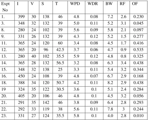
Table 2: Input and Output Parameters and their Objective Function Value
Expt No
I V S T WPD WDR BW RF OF
1. 399 30 138 46 4.8 0.08 7.2 2.6 0.230
2. 416 36 114 28.5 3.9 0.06 9.4 0.7 1.085
3. 348 32 132 39 5.0 0.11 5.2 3.1 0.045
4. 433 20 126 32 3.0 0.06 6.8 2.2 0.578
5. 416 26 138 25 4.2 0.10 6.2 0.6 0582
6. 314 22 126 60 4.6 0.07 8.9 0.5 0.930
7. 297 24 132 42.5 3.2 0.06 7.9 2.4 0.643
8. 280 24 102 39 5.6 0.09 5.8 2.1 0.097
9. 331 26 132 39 4.3 0.12 5.2 1.5 0.277
10. 297 20 102 53 5.2 0.10 9.2 1.9 0.592
11. 365 24 120 60 3.4 0.08 4.5 1.7 0.416
12. 365 20 96 42.5 3.7 0.06 4.7 0.9 0.535
13. 280 40 102 35.5 5.9 0.12 4.8 0.8 0.325
14. 365 28 132 56.5 3.2 0.08 6.3 3.4 0.438
15. 348 32 138 25 3.3 0.11 5.4 3.2 0.344
16. 450 24 108 39 4.8 0.07 6.7 2.9 0.168
Where, WPD = Weld penetration depth; WDR = Weld deposition rate, BW = Bead width; RF = Reinforcement and OF = Objective function value
From Table 2, the welding condition of experiment 3 produced the most satisfactory welding quality, and the welding conditions of experiment number 2 produced the worst quality welds among the initial 16 conditions.
Objective function value of experiment number 3 which is = 0.045 were found to be the minimum objective function value, therefore, for optimization to be reached, an objective function value less than = 0.045 must be attained.
2nd Iteration
In the next step, welding parameter with the greatest objective function value and welding condition with the least objective function value were determined through the results of the experiments on the initial candidate solutions. Three welding conditions were then randomly selected by the controlled random search algorithm from the other fifteen (15) excluding L to comprise a three dimensional simplex and the next search point P was determined by L and the three selected conditions using the equation, . In this equation, is the welding condition selected last, while is the centroid of all the points excluding . For the initial candidate solution, is experiment 2 with objective function value of 1.085 and is experiment 3 with objective function value of 0.045.
Table 3: Table for Second Iteration
Expt No
I V S T WPD WDR BW RF OF
1. 399 30 138 46 4.8 0.08 7.2 2.6 0.230
3. 348 32 132 39 5.0 0.11 5.2 3.1 0.045
4. 433 20 126 32 3.0 0.06 6.8 2.2 0.578
5. 416 26 138 25 4.2 0.10 6.2 0.6 0582
6. 314 22 126 60 4.6 0.07 8.9 0.5 0.930
7. 297 24 132 42.5 3.2 0.06 7.9 2.4 0.643
8. 280 24 102 39 5.6 0.09 5.8 2.1 0.097
9. 331 26 132 39 4.3 0.12 5.2 1.5 0.277
10. 297 20 102 53 5.2 0.10 9.2 1.9 0.592
11. 365 24 120 60 3.4 0.08 4.5 1.7 0.416
12. 365 20 96 42.5 3.7 0.06 4.7 0.9 0.535
13. 280 40 102 35.5 5.9 0.12 4.8 0.8 0.325
14. 365 28 132 56.5 3.2 0.08 6.3 3.4 0.438
15. 348 32 138 25 3.3 0.11 5.4 3.2 0.344
16. 450 24 108 39 4.8 0.07 6.7 2.9 0.168
-17 331 28 108 49.5 4 0.09 7.9 0.8 0.75
The welding conditions which became the next search point obtained from equation are comprised of welding current 331 Amp, welding voltage of 28 V, welding speed 138mm/min and welding time 49.5sec. The weld penetration depth, weld deposition rate, bead width, and reinforcement obtained after welding with this parameters (331Amp, 28V,138mm/min, and 49.5sec) are 4, 0.09, 7.9 and 0.8 respectively with the objective function value of 0.75 which is less than the value of = 1.085. Therefore experiment number 2 corresponding to was eliminated from the candidate solution set, and the welding conditions of point was included (2 left for 17 to come in as shown in Table 3).
3rd Iteration
The welding condition of experiment number 6 now correspond with point with the objective function value of 0.930 and welding condition of experiment 3 corresponds to L with objective function value of 0.045.
Three points generated by the controlled random search algorithm to join experiment 3 in the simplex are experiment 1, 17 and 9. Thus the simplex comprised of the welding conditions of experiments 3, 1, 17 and 9. Experiment 9 being the pole of the experiment. The centroid G was calculated from the points 3, 1, and 17.
Table 4: Table for Third Iteration
Expt No
I V S T WPD WDR BW RF OF
1. 399 30 138 46 4.8 0.08 7.2 2.6 0.230
3. 348 32 132 39 5.0 0.11 5.2 3.1 0.045
4. 433 20 126 32 3.0 0.06 6.8 2.2 0.578
5. 416 26 138 25 4.2 0.10 6.2 0.6 0582
7. 297 24 132 42.5 3.2 0.06 7.9 2.4 0.643
8. 280 24 102 39 5.6 0.09 5.8 2.1 0.097
9. 331 26 132 39 4.3 0.12 5.2 1.5 0.277
10. 297 20 102 53 5.2 0.10 9.2 1.9 0.592
11. 365 24 120 60 3.4 0.08 4.5 1.7 0.416
12. 365 20 96 42.5 3.7 0.06 4.7 0.9 0.535 13. 280 40 102 35.5 5.9 0.12 4.8 0.8 0.325 14. 365 28 132 56.5 3.2 0.08 6.3 3.4 0.438
15. 348 32 138 25 3.3 0.11 5.4 3.2 0.344
16. 450 24 108 39 4.8 0.07 6.7 2.9 0.168
17 331 28 108 49.5 4 0.09 7.9 0.8 0.75
The welding parameters which became the next search point obtained from equation are comprised of welding current 388 Amp, welding voltage 34 V, welding speed 120mm/min and welding time, 50.7sec. The output parameters generated from the welding process are weld penetration depth = 4.2, weld deposition rate 0.11, bead width = 8.2, and reinforcement = 2.9 with an objective function of 0.438 which has a smaller value than the value of = 0.930. Therefore experiment number 6 corresponding to the is eliminated from the candidate solution set, and the welding conditions of point is included (6 left for 18 to come in as shown in Table 4).
4th Iteration
The welding conditions of experiment number 17 correspond with point and the objective function value is 0.750. The welding conditions of experiment number 3 correspond with point , and the objective function value is 0.045. Experiments 3, 15, 18 and 1 are the welding conditions randomly selected to constitute the simplex. The pole of the simplex is the welding parameters of experiment number 1 and the centroid G is calculated from conditions of experiments number 3, 15 and 18.
Table 5: Fourth Iteration
Expt No
I V S T WPD WDR BW RF OF
1. 399 30 138 46 4.8 0.08 7.2 2.6 0.230
3. 348 32 132 39 5.0 0.11 5.2 3.1 0.045
4. 433 20 126 32 3.0 0.06 6.8 2.2 0.578
5. 416 26 138 25 4.2 0.10 6.2 0.6 0582
7. 297 24 132 42.5 3.2 0.06 7.9 2.4 0.643
8. 280 24 102 39 5.6 0.09 5.8 2.1 0.097
9. 331 26 132 39 4.3 0.12 5.2 1.5 0.277
10. 297 20 102 53 5.2 0.10 9.2 1.9 0.592
11. 365 24 120 60 3.4 0.08 4.5 1.7 0.416
12. 365 20 96 42.5 3.7 0.06 4.7 0.9 0.535
13. 280 40 102 35.5 5.9 0.12 4.8 0.8 0.325
14. 365 28 132 56.5 3.2 0.08 6.3 3.4 0.438
15. 348 32 138 25 3.3 0.11 5.4 3.2 0.344
16. 450 24 108 39 4.8 0.07 6.7 2.9 0.168
18. 388 34 120 50.7 4.2 0.11 8.2 2.9 0.438 19. 324 35 122 30.5 3.6 0.1 5.1 2.4 0.284
The welding parameters which became the next search point obtained from equation are comprised of welding current 324 Amp, welding voltage of 35 V, welding speed 122mm/min and welding time, 30.5sec. The weld penetration depth is 3.6, weld deposition rate is 0.1, bead width is 5.1, and reinforcement 2.4 and the objective function value of 0.284 which has a smaller value than the value of = 0.750. Therefore experiment number 17 which correspond with , is eliminated from the candidate solution set and the welding conditions of experiment number 19 which is is included (see Table 5).
Iteration 5
The welding condition of experiment 7 now correspond with point with the objective function value of 0.643 and welding condition of experiment 3 corresponds to L with objective function value of 0.045.
Table.6: Fifth Iteration
Expt No
I V S T WPD WDR BW RF OF
1. 399 30 138 46 4.8 0.08 7.2 2.6 0.230
3. 348 32 132 39 5.0 0.11 5.2 3.1 0.045
4. 433 20 126 32 3.0 0.06 6.8 2.2 0.578
5. 416 26 138 25 4.2 0.10 6.2 0.6 0582
8. 280 24 102 39 5.6 0.09 5.8 2.1 0.097
9. 331 26 132 39 4.3 0.12 5.2 1.5 0.277
10. 297 20 102 53 5.2 0.10 9.2 1.9 0.592
11. 365 24 120 60 3.4 0.08 4.5 1.7 0.416
12. 365 20 96 42.5 3.7 0.06 4.7 0.9 0.535 13. 280 40 102 35.5 5.9 0.12 4.8 0.8 0.325 14. 365 28 132 56.5 3.2 0.08 6.3 3.4 0.438
15. 348 32 138 25 3.3 0.11 5.4 3.2 0.344
16. 450 24 108 39 4.8 0.07 6.7 2.9 0.168
18. 388 34 120 50.7 4.2 0.11 8.2 2.9 0.438
19 324 35 122 30.5 3.6 0.1 5.1 2.4 0.284
20. 405 20 106 46 4.8 0.1 4.5 3.2 0.056
The welding parameters which became the next search point obtained from equation are comprised of welding current 405 Amp, welding voltage of 20 V, welding speed 106mm/min and welding time, 46sec. The output parameters generated from the welding process are weld penetration depth = 4.8, weld deposition rate 0.1, bead width = 4.5, and reinforcement = 3.2 with an objective function of 0.056 which has a smaller value than the value of = 0.643. Therefore experiment number 7 corresponding to the is eliminated from the candidate solution set, and the welding conditions of point is included (7 left for 20 to come in as shown in Table 6).
6th Iteration
The welding condition of experiment 10 now correspond with point with the objective function value of 0.592 and welding condition of experiment 3 corresponds to with objective function value of 0.045.
Table 7: Table of Sixth Iteration
Expt No
I V S T WPD WDR BW RF OF
1. 399 30 138 46 4.8 0.08 7.2 2.6 0.230
3. 348 32 132 39 5.0 0.11 5.2 3.1 0.045
4. 433 20 126 32 3.0 0.06 6.8 2.2 0.578
5. 416 26 138 25 4.2 0.10 6.2 0.6 0582
8. 280 24 102 39 5.6 0.09 5.8 2.1 0.097
9. 331 26 132 39 4.3 0.12 5.2 1.5 0.277
11. 365 24 120 60 3.4 0.08 4.5 1.7 0.416
12. 365 20 96 42.5 3.7 0.06 4.7 0.9 0.535
13. 280 40 102 35.5 5.9 0.12 4.8 0.8 0.325
14. 365 28 132 56.5 3.2 0.08 6.3 3.4 0.438
15. 348 32 138 25 3.3 0.11 5.4 3.2 0.344
16. 450 24 108 39 4.8 0.07 6.7 2.9 0.168
18. 388 34 120 50.7 4.2 0.11 8.2 2.9 0.438
19 324 35 122 30.5 3.6 0.1 5.1 2.4 0.284
20. 405 20 106 46 4.8 0.1 4.5 3.2 0.056
21. 291 35 142 46 3.8 0.09 6.4 2.8 0.293
The welding parameters which became the next search point obtained from equation are comprised of welding current 291 Amp, welding voltage of 35 V, welding speed 142mm/min and welding time, 46sec. The weld penetration depth is 3.8, weld deposition rate is 0.09, bead width is 6.4, and reinforcement 2.8 and the objective function value of 0.293 which has a smaller value than the value of = 0.592. Therefore experiment number 10 which correspond with , is eliminated from the candidate solution set and the welding conditions of experiment number 21 which is is included (see Table 7).
7th Iteration
The welding condition of experiment number 5 now correspond with point with the objective function value of 0.582 and welding condition of experiment 3 corresponds to L with objective function value of 0.045.
Three points generated by the controlled random search algorithm to join experiment 3 in the simplex are experiment 14, 19 and 1. Thus the simplex comprised of the welding conditions of experiments 3, 14, 19 and 1. Experiment 1 being the pole of the experiment. The centroid G is calculated from the points 3, 14, and 19.
Table 8: Table of Seventh Iteration
Expt No I V S T WPD WDR BW RF OF
1. 399 30 138 46 4.8 0.08 7.2 2.6 0.230
3. 348 32 132 39 5.0 0.11 5.2 3.1 0.045
4. 433 20 126 32 3.0 0.06 6.8 2.2 0.578
8. 280 24 102 39 5.6 0.09 5.8 2.1 0.097
9. 331 26 132 39 4.3 0.12 5.2 1.5 0.277
11. 365 24 120 60 3.4 0.08 4.5 1.7 0.416
12. 365 20 96 42.5 3.7 0.06 4.7 0.9 0.535
13. 280 40 102 35.5 5.9 0.12 4.8 0.8 0.325
14. 365 28 132 56.5 3.2 0.08 6.3 3.4 0.438
15. 348 32 138 25 3.3 0.11 5.4 3.2 0.344
16. 450 24 108 39 4.8 0.07 6.7 2.9 0.168
18. 388 34 120 50.7 4.2 0.11 8.2 2.9 0.438 19 324 35 122 30.5 3.6 0.1 5.1 2.4 0.284
20. 405 20 106 46 4.8 0.1 4.5 3.2 0.056
21. 291 35 142 46 3.8 0.09 6.4 2.8 0.293
The welding parameters which became the next search point obtained from equation are comprised of welding current of 292 Amp, welding voltage of 33 V, welding speed 119mm/min and welding time of 38sec. The weld penetration depth is 5.6, weld deposition rate is 0.11, bead width is 7.8, and reinforcement 3 and the objective function value of 0.244 which has a smaller value than the value of = 0.582. Therefore experiment number 5 which correspond with , is eliminated from the candidate solution set and the welding conditions of experiment number 22 which is is included (see Table 8).
8th Iteration
The welding condition of experiment 4 now correspond with point with the objective function value of 0.578 and welding condition of experiment 3 corresponds to with objective function value of 0.045.
Three points generated by the controlled random search algorithm to join experiment 3 in the simplex are experiment 11, 9 and 14. Thus the simplex comprised of the welding conditions of experiments 3, 11, 9 and 14. The pole of the simplex is the welding parameters of experiment number 14 and the centroid G is calculated from parameters of experiments number 3, 11 and 9.
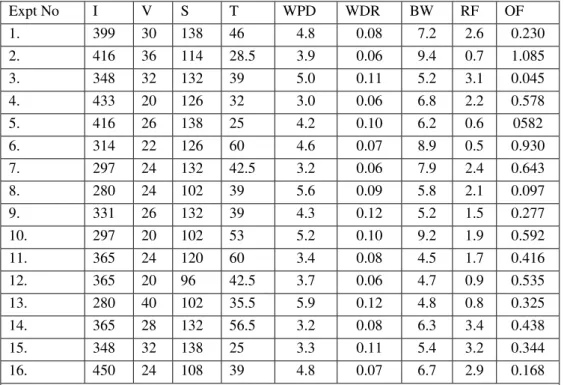
Table 9:Table of Eighth Iteration
Expt No
I V S T WPD WDR BW RF OF
1. 399 30 138 46 4.8 0.08 7.2 2.6 0.230 3. 348 32 132 39 5.0 0.11 5.2 3.1 0.045 8. 280 24 102 39 5.6 0.09 5.8 2.1 0.097 9. 331 26 132 39 4.3 0.12 5.2 1.5 0.277 11. 365 24 120 60 3.4 0.08 4.5 1.7 0.416 12. 365 20 96 42.5 3.7 0.06 4.7 0.9 0.535 13. 280 40 102 35.5 5.9 0.12 4.8 0.8 0.325 14. 365 28 132 56.5 3.2 0.08 6.3 3.4 0.438 15. 348 32 138 25 3.3 0.11 5.4 3.2 0.344 16. 450 24 108 39 4.8 0.07 6.7 2.9 0.168 18. 388 34 120 50.7 4.2 0.11 8.2 2.9 0.438 19 324 35 122 30.5 3.6 0.1 5.1 2.4 0.284 20. 405 20 106 46 4.8 0.1 4.5 3.2 0.056 21. 291 35 142 46 3.8 0.09 6.4 2.8 0.293
22. 292 33 119 38 5.6 0.11 7.8 3 0.244
23. 331 27 124 35.5 5.8 0.1 4.0 2.8 0.010
The welding parameters which became the next search point obtained from equation are comprised of welding current of 331 Amp, welding voltage of 27 V, welding speed 124mm/min and welding time of 35.5secs. The weld penetration depth is 5.8, weld deposition rate is 0.1, bead width is 4.0, and reinforcement 2.8 and the objective function value of 0.010 which has a smaller value than the value of = 0.578. Therefore experiment number 4 which correspond with , is eliminated from the candidate solution set and the welding conditions of experiment number 23 which is is included (see Table 9).
This iteration gives a satisfactory weld quality, since the step 7 have been satisfied which state that stop criterion is satisfied when the value of the objective function is less than a predefined small number of 0.045, then stop; otherwise return to Step 3. Therefore, = 0.01 is the near-optimal value for the optimization since it is less than the minimum value of the objective function obtained from the initial candidate solution.
The final candidate solution consist of welding parameters of experiment numbers 1, 3, 8, 9, 11, 12, 13, 14, 15, 16, 18, 19, 20, 21, 22, and 23 as shown in Table 9
Table 10: Result of Initial Candidate Solutions
Expt No I V S T WPD WDR BW RF OF
1. 399 30 138 46 4.8 0.08 7.2 2.6 0.230
2. 416 36 114 28.5 3.9 0.06 9.4 0.7 1.085
3. 348 32 132 39 5.0 0.11 5.2 3.1 0.045
4. 433 20 126 32 3.0 0.06 6.8 2.2 0.578
5. 416 26 138 25 4.2 0.10 6.2 0.6 0582
6. 314 22 126 60 4.6 0.07 8.9 0.5 0.930
7. 297 24 132 42.5 3.2 0.06 7.9 2.4 0.643
8. 280 24 102 39 5.6 0.09 5.8 2.1 0.097
9. 331 26 132 39 4.3 0.12 5.2 1.5 0.277
10. 297 20 102 53 5.2 0.10 9.2 1.9 0.592
11. 365 24 120 60 3.4 0.08 4.5 1.7 0.416
12. 365 20 96 42.5 3.7 0.06 4.7 0.9 0.535
13. 280 40 102 35.5 5.9 0.12 4.8 0.8 0.325
14. 365 28 132 56.5 3.2 0.08 6.3 3.4 0.438
15. 348 32 138 25 3.3 0.11 5.4 3.2 0.344
16. 450 24 108 39 4.8 0.07 6.7 2.9 0.168
Results of the Next Iteration
17. 331 28 108 49.5 4 0.09 7.9 0.8 0.750
18. 388 34 120 50.7 4.2 0.11 8.2 2.9 0.438
19. 324 35 122 30.5 3.6 0.1 5.1 2.4 0.284
20. 405 20 106 46 4.8 0.1 4.5 3.2 0.056
21. 291 35 142 46 3.8 0.09 6.4 2.8 0.293
22. 292 33 119 38 5.6 0.11 7.8 3 0.244
23. 331 27 124 35.5 5.8 0.1 4.0 2.8 0.01
Findings
The findings of the study are as follows:
A near optimal value was found in the 8th iteration. The welding parameters determined in the 8th iteration as the optimal welding parameters are welding current of 331 Amp, welding voltage of 27 V and welding speed of 124mm/min. The corresponding values of the output parameter of the weld bead geometry are: weld penetration depth is 5.8, weld deposition rate is 0.1, bead width is 4.0, and reinforcement 2.8. The result is satisfactory with the optimal condition found in the 8th iteration even with the slight difference with the established values.
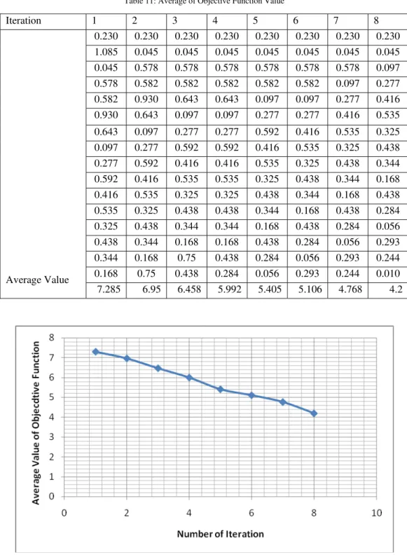
Table 11: Average of Objective Function Value
Figure 1:Chart of decreasing value of objective function obtained from controlled random search procedure iterations
On examination of the chart in Fig. 1, it is seen that the average value of objective functions in the current candidate solutions reduces as iteration proceeds. This occurs as a result of replacing the maximum objective function value with the smaller objective function value that is obtained from subsequent iteration.
The controlled random search algorithm as explained in this work is effective in finding near optimal conditions. However, the convergence performance after reaching near optimal condition diminishes drastically. Therefore, continuing experiment with controlled random search algorithm after finding the near optimal condition is ineffective.
From the data presented and discussed, the output parameters developed by welding with each welding conditions does not follow a general course, therefore, a model cannot be developed between the welding input parameters and the output parameters in the use of controlled random search algorithm.
Iteration 1 2 3 4 5 6 7 8
Average Value
0.230 0.230 0.230 0.230 0.230 0.230 0.230 0.230 1.085 0.045 0.045 0.045 0.045 0.045 0.045 0.045 0.045 0.578 0.578 0.578 0.578 0.578 0.578 0.097 0.578 0.582 0.582 0.582 0.582 0.582 0.097 0.277 0.582 0.930 0.643 0.643 0.097 0.097 0.277 0.416 0.930 0.643 0.097 0.097 0.277 0.277 0.416 0.535
4. Conclusion
In this study the controlled random search method was used to find the near optimal welding parameters and weld bead geometry of a mild steel weldment. Sixteen experimental runs were carried out. For each experimental run, mean values of the measured bead geometry were determined. Also, the corresponding objective functions were determined. The controlled random search method was able to determine a near optimal set of process parameters by determining an objective function lower than the initial or first least objective function value obtained. This low objective function was arrived at after several iterations were made. The near optimal process parameters were found acceptable as they fall within the values found in literature. In this study a step by step approach of using the controlled random search method was followed. It has been discovered that welding process parameters can be effectively optimized using this method when compared with other optimization methods.
References
[1] Achebo, J. I. (2011)’ Optimization of GMAW Protocols and Parameters for Improving Weld Strength Quality’ delivered at the 2011 World Congress on Engineering: International Conference of Manufacturing Engineering and Engineering Management, Imperial College, London , July 6 – 7, 2011 (available online at http://www.iaeng.org/publication/WCE2011/).
[2] Achebo, J.I. (2012) Optimization of Fluence Energy in Relation to Weld Properties based on Vogel Approximation Method. delivered at the 2012 World Congress on Engineering: International Conference on Mechanical Engineering, Imperial College, London , July 4 – 6, 2012 (available online at www.iaeng.org/publication/WCE2012/WCE2012_pp1830-1834.pdf).
[3] Correia, D.S. Goncalves, C.V. Junior, Sebastiao S.C. and Ferraresi, V.A. (2004). GMAW Welding Optimization using genetic Algorithms. J. of the Braz. Soc. of Mech. Sci. and Eng. XXVI (1), pp. 28-33.
[4] Gunaraj, V., and Murugan, N. (1999). Application of response surface methodology for predicting weld bead quality in submerged arc welding of pipes. Journal of Materials Processing Technology 88, pp. 266–275.
[5] Kim, D. Kang, M. and Rhee, S. (2005). Determination of optimal welding conditions with a controlled random search procedure. Supplement to the Welding Journal, August, pp. 125s – 130s.
[6] Pal, S; Malviya, S.K; Pal, S.K and Samantaray, A. K (2009). Optimization of quality characteristic parameters in an pulsed metal inert gas welding process using grey-based Taguchi method. Int. J. Adv. Manuf. Technol. 44, pp. 1250-1260. DOI 10:1007/s00170-009-1931-0.
[7] Patil, S.R. and Waghmare, C.A. (2013). Optimization of MIG welding parameters for improving strength of welded joints. International Journal of Advanced Engineering Research and Studies. 11(IV), pp. 14-16.
[8] Sreeraj, P., Kannan, T. and Maji, S. (2013). Prediction and Optimization of weld bead geometry in Gas Metal Arc Welding process using RSM and fmincon. Journal of Mechanical Engineering Research. 5 (8), pp. 154 – 265. DOI: 10:5897/JMER 2013.0292. [9] Sudhakaran R., Senthil Kumar K. M. [2011] Effect of Welding Process Parameters on Weld Bead Geometry and Optimization of
Process Parameters to Maximize Depth to Width Ratio for Stainless Steel Gas Tungsten Arc Welded Plates Using Genetic Algorithm, European Journal of Scientific Research, 62 (1), pp.76-94
Appendix: CRS Search Code
Public Class Form1
Dim Crs_table AsNew Dictionary(OfInteger, Single)
Dim Vup, Vlo, Iup, Ilo, Fup, Flo, Tup, Tlo, Tin AsSingle Dim DeHeight, DeWidth, DePenetration AsSingle
Dim count AsInteger : Dim var_list AsNew Dictionary(OfString, Single)
PrivateSub GroupBox1_Enter(sender AsObject, e As EventArgs) Handles GroupBox1.Enter
EndSub
PrivateSub Table1BindingNavigatorSaveItem_Click(sender AsObject, e As EventArgs) Handles
Table1BindingNavigatorSaveItem.Click
Me.Validate()
Me.Table1BindingSource.EndEdit()
Me.TableAdapterManager.UpdateAll(Me.Database1DataSet)
EndSub
PrivateSub Form1_Load(sender AsObject, e As EventArgs) HandlesMyBase.Load
'TODO: This line of code loads data into the 'Database1DataSet.Table1' table. You can move, or remove it, as needed.
EndSub
PrivateSub Table1_CellContentClick(sender AsObject, e As DataGridViewCellEventArgs) Handles
Table.CellContentClick
EndSub
PrivateSub crs_ini() ' suplies value to the dictionary and other needed variable
With Table
For i AsInteger = 0 To .RowCount - 2
Crs_table.Add(.Item(0, i).Value, .Item(7, i).Value)
Next EndWith
Vup = CSng(txtVup.Text) Vlo = CSng(txtVlo.Text) Iup = CSng(txtCup.Text) Ilo = CSng(txtClo.Text) Fup = CSng(txtFup.Text) Flo = CSng(txtFlo.Text) Tup = CSng(txtTimeUp.Text) Tlo = CSng(txtTimeLo.Text) Tin = CSng(txtTimeInterval.Text) DeHeight = CSng(TextBox6.Text) DeWidth = CSng(txtObjLo.Text) DePenetration = CSng(TextBox8.Text)
EndSub
PrivateSub crs()
1: Dim list AsNew List(OfInteger) list.Clear()
Dim ran AsNew Random
' TextBox1.AppendText(ran.NextDouble & vbCrLf)
TextBox1.AppendText(Crs_table.Values.Min & vbCrLf)
Dim min = Crs_table.Values.Min
Dim key AsInteger
ForEach item In Crs_table
If item.Value = min Then
key = item.Key list.Add(key)
EndIf Next
TextBox1.AppendText(" min key "& key & vbCrLf)
For i AsInteger = 0 To 2
Dim tem AsInteger = key
DoUntil (tem <> key And list.Contains(tem) = False)
tem = ran.Next(Crs_table.Keys.Min, Crs_table.Keys.Max + 1)
Loop
Next
Dim meanF = (CSng(Table.Item(1, list(0)).Value) + CSng(Table.Item(1, list(1)).Value) + CSng(Table.Item(1, list(2)).Value)) / 3
Dim meanV = (CSng(Table.Item(2, list(0)).Value) + CSng(Table.Item(2, list(1)).Value) + CSng(Table.Item(2, list(2)).Value)) / 3
Dim meanS = (CSng(Table.Item(3, list(0)).Value) + CSng(Table.Item(3, list(1)).Value) + CSng(Table.Item(3, list(2)).Value)) / 3
Dim meanT = (CSng(Table.Item(4, list(0)).Value) + CSng(Table.Item(4, list(1)).Value) + CSng(Table.Item(4, list(2)).Value)) / 3
Dim F = meanF * 2 - Table.Item(1, list(3)).Value
Dim V = meanV * 2 - Table.Item(2, list(3)).Value
Dim S = meanS * 2 - Table.Item(3, list(3)).Value
Dim T = meanT * 2 - Table.Item(4, list(3)).Value
TextBox1.AppendText("v = "& V &" F = "& F &" S = "& S & vbCrLf)
ForEach item In Crs_table
TextBox1.AppendText(item.Key &" "& item.Value & vbCrLf)
Next
TextBox1.AppendText(" list of random keys"& vbCrLf)
ForEach item In list
TextBox1.AppendText(item & vbCrLf)
Next
count = Math.Abs(Table.Item(10, Table.RowCount - 2).Value) + 1
Database1DataSet.Tables(0).Rows.Add(count, F, V, S, T, Nothing, Nothing, Nothing) var_list.Clear()
EndSub
PrivateSub Example()
Database1DataSet.Table1.Clear()
With Database1DataSet.Tables(0).Rows .Add(1, 20.4, 19, 8, 2.0, 0.0, 1.5, 28.5) .Add(2, 19.1, 24, 5, 1.2, 4.6, 5.0, 0.5) .Add(3, 16.5, 21, 7, 1.7, 0.0, 3.7, 17.7) .Add(4, 13.9, 18, 9, 0.5, 0.0, 1.5, 29.3) .Add(5, 17.8, 19, 3, 3.2, 0.0, 2.2, 26.7) .Add(6, 12.6, 21, 6, 1.8, 0.0, 2.5, 22.3) .Add(7, 11.3, 23, 6, 1.5, 0.0, 2.0, 23.8) .Add(8, 15.2, 20, 4, 2.0, 3.6, 5.0, 0.4) .Add(9, 21.7, 20, 9, 1.4, 0.0, 1.0, 32.0) .Add(10, 16.5, 21, 7, 2.1, 0.0, 3.0, 20.4)
EndWith EndSub
PrivateFunction obj(ByVal i AsInteger) AsSingle
obj = ((DeHeight - CSng(Table.Item(4, i).Value) ^ 2) + (DeWidth - CSng(Table.Item(5, i).Value) ^ 2) + (DePenetration - CSng(Table.Item(6, i).Value) ^ 2))
PrivateSub Button3_Click(ByVal sender As System.Object, ByVal e As System.EventArgs) Handles
Button3.Click
Me.Database1DataSet.Table1.Clear()
EndSub
PrivateSub Button2_Click(ByVal sender As System.Object, ByVal e As System.EventArgs) Handles
Button2.Click
Me.Validate()
Me.Table1BindingSource.EndEdit()
Me.TableAdapterManager.UpdateAll(Me.Database1DataSet)
EndSub
PrivateSub Table1BindingNavigatorSaveItem_Click_1(ByVal sender As System.Object, ByVal e As
System.EventArgs)
Me.Validate()
Me.Table1BindingSource.EndEdit()
Me.TableAdapterManager.UpdateAll(Me.Database1DataSet)
EndSub
PrivateSub Table1BindingNavigatorSaveItem_Click_2(ByVal sender As System.Object, ByVal e As
System.EventArgs)
Me.Validate()
Me.Table1BindingSource.EndEdit()
Me.TableAdapterManager.UpdateAll(Me.Database1DataSet)
EndSub
PrivateSub Table1BindingNavigator_RefreshItems(ByVal sender As System.Object, ByVal e As
System.EventArgs)
EndSub
PrivateSub Button4_Click(ByVal sender As System.Object, ByVal e As System.EventArgs) Handles
Button4.Click Example()
EndSub
PrivateSub Button1_Click(ByVal sender As System.Object, ByVal e As System.EventArgs) Handles
Button1.Click crs_ini()
EndSub
PrivateSub Button6_Click(ByVal sender As System.Object, ByVal e As System.EventArgs) Handles
Button6.Click crs()
PrivateSub Button7_Click(ByVal sender As System.Object, ByVal e As System.EventArgs) Handles
Button7.Click
Dim listC, listV, listS AsNew List(OfDouble) : Dim ran AsNew Random Randomize()
Dim val, lim1 AsDouble
Vup = CSng(txtVup.Text) Vlo = CSng(txtVlo.Text) Iup = CSng(txtCup.Text) Ilo = CSng(txtClo.Text) Fup = CSng(txtFup.Text) Flo = CSng(txtFlo.Text)
lim1 = Vup
val = CDbl(txtVlo.Text)
DoUntil (val > lim1)
listV.Add(val)
val += CDbl(txtVint.Text)
If val = lim1 Then
listV.Add(val)
EndIf Loop
val = 0 lim1 = Iup
val = CDbl(txtClo.Text)
DoUntil (val > lim1)
listC.Add(val)
val += CDbl(txtCint.Text)
If val = lim1 Then
listC.Add(val)
EndIf
Loop
val = 0 lim1 = Fup
val = CDbl(txtFlo.Text)
DoUntil (val > lim1)
listS.Add(val)
val += CDbl(txtFint.Text)
If val = lim1 Then
listS.Add(val)
EndIf Loop
val = 0
Dim k, l, m AsInteger
For i AsInteger = 0 ToCInt(txtSample.Text)
l = ran.Next(1, listS.Count) m = ran.Next(0, listC.Count)
count = Math.Abs(Table.Item(0, Table.RowCount - 1).Value) + 1
Database1DataSet.Tables(0).Rows.Add(count, listC.Item(m), listV.Item(k), listS.Item(l), Nothing,
Nothing, Nothing, Nothing)
Next EndSub
PrivateSub Button8_Click(ByVal sender As System.Object, ByVal e As System.EventArgs) Handles
Button8.Click
Dim objV AsSingle
For i AsInteger = 0 To Table.RowCount - 1
If Table.Item(0, i).Value = TextBox2.Text Then
objV = obj(i)
Table.Item(7, i).Value = objV
EndIf Next EndSub
PrivateSub Button5_Click(ByVal sender As System.Object, ByVal e As System.EventArgs) Handles
Button5.Click
Dim objV AsSingle
For i AsInteger = 0 To Table.RowCount - 1
objV = obj(i)
Table.Item(7, i).Value = objV
Next EndSub
PrivateSub Button9_Click(ByVal sender As System.Object, ByVal e As System.EventArgs) Handles
Button9.Click
IfCSng(txtSample.Text) < 2 Then
MsgBox("Sample size not specified")
Exit Sub EndIf
For i AsInteger = 0 To Table.RowCount - 1
If Table.Item(5, i).Value = ""Then
MsgBox("Data not properly entered")
Exit Sub EndIf
Next
For i AsInteger = 0 To Table.RowCount - 1 ' Updating crs_table
If Crs_table.Keys.Contains(Table.Item(0, i).Value) = FalseThen
Crs_table.Add(Table.Item(0, i).Value, Table.Item(7, i).Value)
EndIf Next
Dim max AsSingle : Dim maxk AsInteger
For i AsInteger = CInt(txtSample.Text) To Crs_table.Count - 1
For j AsInteger = 0 To Crs_table.Count - 1
If max = Crs_table.Values(j) Then
maxk = Crs_table.Keys(j)