Global scale modeling of melting and isotopic evolution of Earth's mantle

(1)

GMDD

8, 9553–9587, 2015

Global scale modeling of melting

and isotopic evolution of Earth’s

mantle

H. J. van Heck et al.

Title Page

Abstract Introduction

Conclusions References

Tables Figures

◭ ◮

Back Close

Full Screen / Esc

Printer-friendly Version

Interactive Discussion

Discussion

P

a

per

|

Discussion

P

a

per

|

Discussion

P

a

per

|

Discussion

P

a

per

|

Geosci. Model Dev. Discuss., 8, 9553–9587, 2015 www.geosci-model-dev-discuss.net/8/9553/2015/ doi:10.5194/gmdd-8-9553-2015

This discussion paper is/has been under review for the journal Geoscientific Model Development (GMD). Please refer to the corresponding final paper in GMD if available.

Global scale modeling of melting and

isotopic evolution of Earth’s mantle

H. J. van Heck1,2, J. H. Davies1, T. Elliott3, and D. Porcelli4

1

School of Earth and Ocean Sciences, CardiffUniversity, Main Building, Park Place, Cardiff, CF10 3AT, Wales, UK

2

Department of Earth Sciences, Utrecht University, Heidelberglaan 2, 3584 CS Utrecht, the Netherlands

3

Department of Earth Sciences, University of Bristol, Wills Memorial Building, Queen’s Road, Bristol BS8 1RJ, UK

4

Department of Earth Sciences, University of Oxford, South Parks Road, Oxford OX1 3AN, UK

Received: 21 August 2015 – Accepted: 28 August 2015 – Published: 3 November 2015

Correspondence to: H. J. van Heck ([email protected])

(2)

GMDD

8, 9553–9587, 2015

mantle

Title Page

Tables Figures

◭ ◮

Back Close

Full Screen / Esc

Discussion

P

a

per

|

Discussion

P

a

per

|

Discussion

P

a

per

|

Discussion

P

a

per

|

Abstract

Many outstanding problems in solid Earth science relate to the geodynamical explana-tion of geochemical observaexplana-tions. Currently, extensive geochemical databases of sur-face observations exist, but satisfying explanations of underlying mantle processes are lacking. One way to address these problems is through numerical modelling of mantle 5

convection while tracking chemical information throughout the convective mantle. We have implemented a new way to track both bulk compositions and concentrations of trace elements in a finite element mantle convection code. Our approach is to track bulk compositions and trace element abundances via particles. One value on each particle represents bulk composition, and can be interpreted as the basalt component. 10

In our model, chemical fractionation of bulk composition and trace elements happens at self-consistent, evolving melting zones. Melting is defined via a composition-dependent solidus, such that the amount of melt generated depends on pressure, temperature and bulk composition of each particle. A novel aspect is that we do not move particles that undergo melting; instead we transfer the chemical information carried by the particle 15

to other particles. Molten material is instantaneously transported to the surface layer, thereby increasing the basalt component carried by the particles close to the surface, and decreasing the basalt component in the residue.

The model is set to explore a number of radiogenic isotopic systems but as an exam-ple here the trace elements we choose to follow are the Pb isotopes and their radioac-20

tive parents. For these calculations we will show: (1) The evolution of the distribution of bulk compositions over time, showing the build up of oceanic crust (via melting-induced chemical separation in bulk composition); i.e. a basalt-rich layer at the surface, and the transportation of these chemical heterogeneities through the deep mantle. (2) The amount of melt generated over time. (3) The evolution of the concentrations 25

(3)

GMDD

8, 9553–9587, 2015

mantle

Title Page

Tables Figures

◭ ◮

Back Close

Full Screen / Esc

Discussion

P

a

per

|

Discussion

P

a

per

|

Discussion

P

a

per

|

Discussion

P

a

per

|

1 Introduction

A big question in solid Earth sciences is: What are the interior dynamics of the mantle? A related question that might help to find answers is: What processes are respon-sible for the geochemical heterogeneity observed in magmatic outputs (recorded in databases, e.g. Lehnert et al., 2000). Some aspects of the geochemical observations 5

are constraints on mantle dynamics, because the dynamics are partly responsible for the heterogeneity in geochemical observations. Therefore progress can be made by introducing geochemistry to (numerical) mantle convection models (as in Christensen and Hofmann, 1994; van Keken and Ballentine, 1998; Xie and Tackley, 2004a; Huang and Davies, 2007b; Brandenburg et al., 2008).

10

In the Earth’s mantle, chemical heterogeneities in bulk composition and trace el-ement concentration and isotope composition are continuously created by melting. Oceanic crust is produced by partial melting at oceanic spreading centres where most mantle melting occurs, and also where most chemical heterogeneity is generated. This heterogeneous material is brought into the deeper mantle via subduction of oceanic 15

lithosphere. Here it mixes. To a lesser extent, melting also happens on continents and beneath oceanic lithosphere to create ocean island basalts (OIB), providing a sec-ond mechanism for creating heterogeneity. This makes melting a first order feature to be implemented in thermo-chemical convection codes. In addition to this continuous generation of heterogeneities, chemically distinct material might have survived for bil-20

lions of years, originating much earlier in Earth history e.g. linked to core formation processes, mantle magma oceans, or asteroid bombardment.

Numerical mantle convection codes have been developed that are capable of track-ing chemical heterogeneities (for an overview see Tackley, 2007). Although different techniques each have advantages (level-set Samuel and Evonuk, 2010, field tracking 25

(4)

GMDD

8, 9553–9587, 2015

mantle

Title Page

Tables Figures

◭ ◮

Back Close

Full Screen / Esc

Discussion

P

a

per

|

Discussion

P

a

per

|

Discussion

P

a

per

|

Discussion

P

a

per

|

In this paper, we will deal with global scale convection, melting, and the tracking of heterogeneities resulting from melting. Christensen and Hofmann (1994) were the first to demonstrate a method to track the evolution of recycled oceanic crust and its influence on the chemistry of the mantle. After that study was published, many fol-lowed a similar approach, either tracking preset heterogeneities (e.g. Davies, 2002; 5

Zhong and Hager, 2003; Nakagawa and Tackley, 2004), or having the chemical het-erogeneities emerge via melting during the calculation at fixed melting zones (Walzer and Hendel, 1999; Davies, 2002; Huang and Davies, 2007a, b, c), moving melting zones that follow force-balanced plates or imposed plate motions (Brandenburg and van Keken, 2007a; Brandenburg and Van Keken, 2007b; Brandenburg et al., 2008), 10

or freely moving melting location via a melting phase diagram (De Smet et al., 1998; Van Thienen et al., 2004; Xie and Tackley, 2004a, b; Nakagawa et al., 2009, 2010).

In addition to tracking of bulk compositions, it is also possible to track the distribution and evolution of trace element abundances. Of particular interest are both parent and daughter isotopes of radiogenic systems. Since the radiogenic parents decay in a very 15

predictable manner (following known decay constants) their relative abundances com-pared to their daughter isotopes can be used as clocks. Different elements behave di_fferently during partial melting (via di_fferent partition coe_fficients), so when the tech-niques of tracking and melting are implemented the system of segregation and decay can be tracked. We follow the well studied Uranium–Thorium–Lead system (U-Th-Pb), 20

as has previously been done in a similar way in: Christensen and Hofmann (1994); Xie and Tackley (2004a); Brandenburg et al. (2008).

For purely thermal convection, numerous analytical solutions exist, which can be used to benchmark numerical codes. (For example Rayleigh–Taylor instabilities; Nu-Ra scalings; corner flow.) In this way, numerical codes can be checked for accuracy 25

(5)

GMDD

8, 9553–9587, 2015

mantle

Title Page

Tables Figures

◭ ◮

Back Close

Full Screen / Esc

Discussion

P

a

per

|

Discussion

P

a

per

|

Discussion

P

a

per

|

Discussion

P

a

per

|

use this theory and compare its predictions to the outcome of newly performed numer-ical calculations.

In this paper, we present the details of a newly implemented method of melt and chemical heterogeneity tracking in a global scale convection code. We will show a good fit of our model data to the analytical prediction of Pb-isochron ages as function of 5

melting age distribution functions. Through this we validate our implementation.

2 Methods

In this section we first describe the numerical code and calculation setup before pre-senting more details about using particles to track bulk and trace element compositions. Then we move on to describe the implementation of melting, including changes in man-10

tle bulk compositions and fractionation of trace elements. We conclude this section by providing some details about the initial setup of the trace elements, as done for the calculation presented.

2.1 Fluid flow convection

We use TERRA, a parallel, well-established, benchmarked, spherical convection code 15

(6)

GMDD

8, 9553–9587, 2015

mantle

Title Page

Tables Figures

◭ ◮

Back Close

Full Screen / Esc

Discussion

P

a

per

|

Discussion

P

a

per

|

Discussion

P

a

per

|

Discussion

P

a

per

|

Assuming incompressibility and the Boussinesq approximation the equations for con-vective flow in the mantle can be expressed non-dimensionally as:

∇ ·u=0, (1)

∇ ·(µ(u_i,j+uj,i))− ∇p=RaTeˆ, (2)

∂T

∂t +∇ ·(Tu)=∇

2_T

+H′ ₍₃₎

5

where length is non-dimensionalised by D the depth of the mantle; time is non-dimensionalised byD2κ−1(κ the thermal di_ffusivity), and temperature by△T the tem-perature drop across the domain.

The other variables and parameters are; u velocity, µ dynamic viscosity, p pres-sure, T temperature, ˆe the radial unit vector,Ra the Rayleigh number (=αρg△T D

3

µκ ;α

10

thermal expansion,ρ reference density,g gravity acceleration),t time,H′ is the non-dimensional internal heating, equal to: _ρcH

p, whereH is the heat generation rate per unit volume andcp is the specific heat at constant pressure. Material movement is driven by buoyancy forces resulting from horizontal differences in density as expressed in the momentum equation (Eq. 2). Temperature is advected with the material flow, diffuses 15

and is produced internally as described by Eq. (3); Eq. (3) describes the advection of temperature with the material flow, and its diffusion, and the heat produced internally; while Eq. (1) is the continuity equation which ensures conservation of mass. Equa-tions (1) and (2) are solved using finite elements, while Eq. (3) is solved via a finite volume method.

20

2.2 Calculation setup

Resolution was chosen such that radial resolution was∼22 km. Lateral resolution was

(7)

GMDD

8, 9553–9587, 2015

mantle

Title Page

Tables Figures

◭ ◮

Back Close

Full Screen / Esc

Discussion

P

a

per

|

Discussion

P

a

per

|

Discussion

P

a

per

|

Discussion

P

a

per

|

ity increased by a factor of 30 at a depth of 660 km. Dimensional values used are listed in Table 1.

To mimic most of Earth’s evolution we ran the calculation over a time corresponding to several billions of years. The calculation started at a time 3.6 Ga and ran forward until present day. By doing so we skip the first billion year of the Earth’s evolution. This is 5

done because in Earth’s early evolution, mantle temperatures were most likely higher than they are at present, leading to lower viscosity and higher vigour in the convection. Numerically this type of convection would be harder to solve for accurately. Moreover, the style of convection and so whether or not it can be treated using the same sort of model is also uncertain. We note that the viscosity is not temperature-dependent in the 10

actual simple case presented here, and so the starting time could be older.

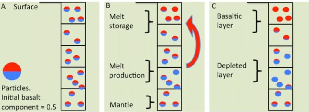
2.3 Particles and bulk composition

We use particles for tracking chemical information, and thus for dealing with melting. A schematic illustration of how this works is given in Fig. 1. The particles are advected using a second order Runge–Kutta advection scheme. Each particle is linked to an 15

array to carry the particle information. Three values are used to indicate the particles position; one to indicate the mass that the particle represents; one to track at what time the particle last produced or received melt; one to track the bulk composition; and one for the abundance of each isotope which is tracked in the system. Using the setup presented in this paper that means that each particle is linked to an array with 13 num-20

bers. The mass that a particle represents is attributed at initialisation as the volume of the node, multiplied by the density, divided by the number of particles attributed to that node. After initialisation, the mass a particle represents is only changed when the particle is split, or merged with another particle (i.e. for numerical, not physical rea-sons. See Sect. 2.4 for more details.). Bulk composition is tracked by a single number 25

(8)

sec-GMDD

8, 9553–9587, 2015

mantle

Title Page

Tables Figures

◭ ◮

Back Close

Full Screen / Esc

Discussion

P

a

per

|

Discussion

P

a

per

|

Discussion

P

a

per

|

Discussion

P

a

per

|

tion above. This includes on initialisation giving all particles a value of 0.6, representing a homogeneous partly fertile mantle.

2.4 Splitting and merging

In order to keep proper coverage of particles throughout the mantle, we sometimes need to split and merge particles. Particles were split whenever less than a threshold 5

number of particles are present in a grid cell. The threshold for the calculations pre-sented here was three. All particles in such cells are split in half, creating two new particles each representing half the original mass. One particle copies the position of the old particle while the other is placed in the same grid cell, mirrored over thez axis. Each new particle receives half of the atoms of each isotope the old particle was car-10

rying, while bulk composition and melting time are simply copied.

Merging of particles is needed sometimes as well. The threshold number of particles required in a grid cell before merging was undertaken can again be varied and was set at 35 in the calculations presented here. When 2 particles merge, their mass and isotopes are simply summed. Which 2 particles are merged is determined by their 15

location in the array allocated to the node, so effectively they are selected ad random. The position of the new particles is the average location determined by weighting the old positions according to the particle masses. The bulk composition is also the mass weighted average of the two original compositions. The melting time of the new particle is copied from one of the old particles picked at random. We note that these rules 20

for splitting and merging particles conserves the global bulk composition, mass and isotope abundances.

2.5 Trace elements

We track the evolution of different trace elements through the domain, focussing on sev-eral isotopes of Uranium (U), Thorium (Th) and Lead (Pb).238U, 235U, and232Th are 25

(9)

GMDD

8, 9553–9587, 2015

mantle

Title Page

Tables Figures

◭ ◮

Back Close

Full Screen / Esc

Discussion

P

a

per

|

Discussion

P

a

per

|

Discussion

P

a

per

|

Discussion

P

a

per

|

208

Pb are produced as ultimate decay products.The ratios of these radiogenic (daugh-ter) isotopes to the non-radiogenic 204Pb change as a function of time and parent-daughter ratios. For206Pb/204Pb and207Pb/204Pb, changes of parent-daughter ratios are coupled, since both have parent U isotopes,238U and235U respectively. Thus man-tle sources, in which U is variably fractionated from Pb, evolve to different206Pb/204Pb 5

and 207Pb/204Pb with time, but the slope of the correlation between these two ratios defines the time of U-Pb fractionation. In reality, it is unlikely the mantle comprises dis-crete reservoirs, fractionated at the same time and more plausibly a mixture of sources fractionated at variable times. In this case the slope of an array of206Pb/204Pb and

207

Pb/204Pb ratios for mantle-derived samples still carries age information about man-10

tle evolution (e.g. Allègre et al., 1980), but interpretation of such “pseudo-isochrons” (see Rudge, 2006) is more complex. One potassium isotope (40K) is also tracked since, next to U and Th,40K is the isotope that generates the bulk of the mantle’s internal heating.

For all radioactive parents we first estimate the total amount of each isotope at 15

present day. That is the amount in all reservoirs combined, i.e. the total budget for the Earth. After that is done, we estimate the amount at the start of the calculation (3.6 Ga ago) by adding the amount that has decayed since then, via standard expo-nential decay (Eq. 4):

Xs=Xpd×e△t×λ (4)

20

whereX can be either U, Th, or K;Xs is the abundance at the start of the calculation;

Xpd the abundance at present day;λis the decay constant, and△tis the time between

the time at the start and present day.

2.6 Melting

We now describe the melting algorithm starting with an overview. The melting algorithm 25

(10)

GMDD

8, 9553–9587, 2015

mantle

Title Page

Tables Figures

◭ ◮

Back Close

Full Screen / Esc

Discussion

P

a

per

|

Discussion

P

a

per

|

Discussion

P

a

per

|

Discussion

P

a

per

|

melt and its content of trace elements is calculated for each such particle. This informa-tion is then passed to near surface particles conserving energy, mass, bulk composiinforma-tion and atoms of trace elements. Note that, in contrast to many other implementations, the melting particles are not moved as part of the melting event. We next describe the gen-eral assumptions underlying our algorithm, and then describe the specific choices and 5

give more details.

Our melting relationships follow from 3 assumptions. The first assumption is that the proportion of fusible (or basaltic) material in a particle can be represented by a compo-sitional parameterC. Following a melting event, all or part of this fusible component is removed from the melt-producing particle, thereby depleting it. The degree of melting, 10

F, is given directly by the change in compositionCas follows,

F =Co−Cn, (5)

where, Cn is the new bulk composition and Co is the previous bulk composition, as

recorded at the particle.

The second assumption is that the solidus is dependent on the compositional pa-15

rameter,C. i.e.Ts=f(C), whereTsis the solidus temperature, andf(C) is a function of

C. Physically the functionf(C) must be monotonic, i.e. the solidus temperature must increase steadily as the composition becomes more depleted. Since f(C) is mono-tonic, its inverse function,f−1=g(Ts) (also monotonic) exists. The functionggives the

composition,C, as a function of the solidus temperatureC=g(Ts).

20

The third assumption is that, following the melting event the temperature of the par-ticle will be the temperature of the solidus for its new composition; this is achieved by changing the composition, not the temperature. Melt can be extracted until the residual composition is so refractory (C=0), that no further melting occurs.

Using these assumptions, the degree of melting is explicitly calculated as follows. 25

(11)

GMDD

8, 9553–9587, 2015

mantle

Title Page

Tables Figures

◭ ◮

Back Close

Full Screen / Esc

Discussion

P

a

per

|

Discussion

P

a

per

|

Discussion

P

a

per

|

Discussion

P

a

per

|

actual temperature on the particle, we calculate the new composition of the residue

Cn (assuming it is in thermal equilibrium with its new solidus (T); and only when the

temperature exceeds the solidus.)

Cn=C(T). (6)

Then using Eq. (5) we can calculate the degree of melting,F, using the new compo-5

sition. For numerical reasons we set a threshold forF of at least 0.0001; degrees of melting lower than this are ignored.

For this work we make the simplifying assumption that the functions relating solidus temperature to composition and the inverse are linear; i.e. functionsf andgare linear. This simplification is justified for this work since our goal is to demonstrate and then 10

test the method with a simple semi-analytical model. We also assume that the solidus temperature is a function of pressure, and make the reasonable, simplifying assumption for this work, that it is a linear relationship (see Fig. 2). As a result we get that

Cn=1−

T−(Tm₋1+z×dTm/dz) △TComp

, (7)

where,C_nis the new bulk composition;T the temperature at the particle;T_m₋₁the melt-15

ing temperature at the surface for material of composition ofC=1;z the depth of the particle; dTm/dz the slope of the solidus; and △TComp the compositionally dependent

temperature difference between the solidii for material of composition zero and material of composition one.

The total amount of melt is calculated by multiplying the mass of the particle with 20

(12)

GMDD

8, 9553–9587, 2015

mantle

Title Page

Tables Figures

◭ ◮

Back Close

Full Screen / Esc

Discussion

P

a

per

|

Discussion

P

a

per

|

Discussion

P

a

per

|

Discussion

P

a

per

|

such that a layer of pure basalt forms and all the melt is accommodated. Since not all particles represent the same amount of mass, we are careful to ensure that all melt is stored and mass conservation is obeyed. Note that the melting/residue particle keeps the same mass. This reflects the fact that the melting column subsides (compacts) in the following way: Since basalt is removed, and the particle’s mass is conserved, 5

the removed material is implicitly replaced by depleted material (of compositionC=0, because fusible component is linearly linked to degree of melting, Eq. 5). The basalt is stored higher in the column, where it takes the space of fully depleted material. Any intervening layers are unchanged.

Note, after melting that while the temperature of the melt producing particle in the 10

residue is unchanged (and hence energy is conserved in the melting event), it is in ther-mal equilibrium with its new solidus since its composition has changed appropriately. The implementation presented here does not take the effect of latent heat or thermal advection by melt migration into account. Neglecting this will only have an e_ffect on the thermal evolution of calculations, and then only ones with massive magmatism. The 15

effect on the chemical evolution, considered here, will be minimal. This aspect could be added to the model if future applications required it.

We then bring the trace isotopes with the melt to the surface. For this we assume simple batch melting partitioning,

Am−i=F×

As−i

F +(D_i×(1−F)), (8) 20

whereAm−i is the abundance of isotopei [number of moles] that is moved to the melt;

As₋i the abundance that was present in the solid before melting; F is the degree of melting (Eq. 5); and Di the isotope (and element) specific partition coefficient. Note that the right hand side starts with a multiplication withF, which is not needed when elemental fractionation is described in terms of concentrations. Since our approach 25

(13)

GMDD

8, 9553–9587, 2015

mantle

Title Page

Tables Figures

◭ ◮

Back Close

Full Screen / Esc

Discussion

P

a

per

|

Discussion

P

a

per

|

Discussion

P

a

per

|

Discussion

P

a

per

|

We define a melting age for each particle. This is the most recent time that a particle changes its bulk composition due to melting, either by producing or receiving melt. The particles track their melting age, saving this time as one of their attributes.

2.7 Initialisation of chemistry

The bulk composition is initialised with a C value (bulk composition) of 0.6 for each 5

particle. The initialisation of trace elements is done in terms of concentrations, once attributed to the particles these concentrations are translated to abundances via the masses of the particles. At initialisation we homogeneously depleted the top 30 % of the mantle in all trace elements to 98 %. This was done as an end-member model (e.g. Armstrong, 1968) to account for the removal of heat-forming elements to the continen-10

tal crust before 3.6 Ga. We thus implicitly assume that fluxes to the continental crust are balanced by fluxes back to the mantle, although we do not explicitly model this process or its potentially heterogeneous distribution.

2.7.1 Radioactive parents

Uranium-238 (238U) is initialised via an estimate of238U (mole gram−1) for the present 15

Bulk Silicate Earth.235U is initialised via the present day molar ratio of238U/235U.40K and232Th abundances are estimated via their present day mass ratios to238U. Values used are listed in the Table 2 and expressed algebraically as:

235

Upd=238Upd/U238U235pd, (9)

40

Kpd= 40

K%

100 ×

238

Upd×KUMR×

M(U)

M(K), (10)

20

232_Th

pd=238Upd×ThUMR×

M(U)

(14)

GMDD

8, 9553–9587, 2015

mantle

Title Page

Tables Figures

◭ ◮

Back Close

Full Screen / Esc

Discussion

P

a

per

|

Discussion

P

a

per

|

Discussion

P

a

per

|

Discussion

P

a

per

|

2.7.2 Radioactive daughters

The BSE abundance of204Pb is estimated via the molar ratio to 238U at present day. Note that, since204Pb is stable, this equals the amount at the start of a calculation.

204

Pb=238Upd/U238Pb204pd. (12)

Initial abundances for the radiogenic Pb isotopes are estimated via the ratio to204Pb 5

at time of the formation of Earth:

206_Pb

s=204Pb×Pb 206/204 diablo +

238_U

D, (13)

207_Pb

s=204Pb×Pb 207/204 diablo +

235_U

D, (14)

208

Pbs=204Pb×Pb 208/204 diablo +

232

ThD. (15)

The238U_D,235U_D,232Th_D are the amounts of 238U, 235U, and 232Th respectively that 10

have decayed between the formation of the Earth and the time the calculation starts (3.6 Ga). These values are calculated using Eq. (4), withTE, the age of the Earth, and

the decay constants as listed in Table 3.

3 Results

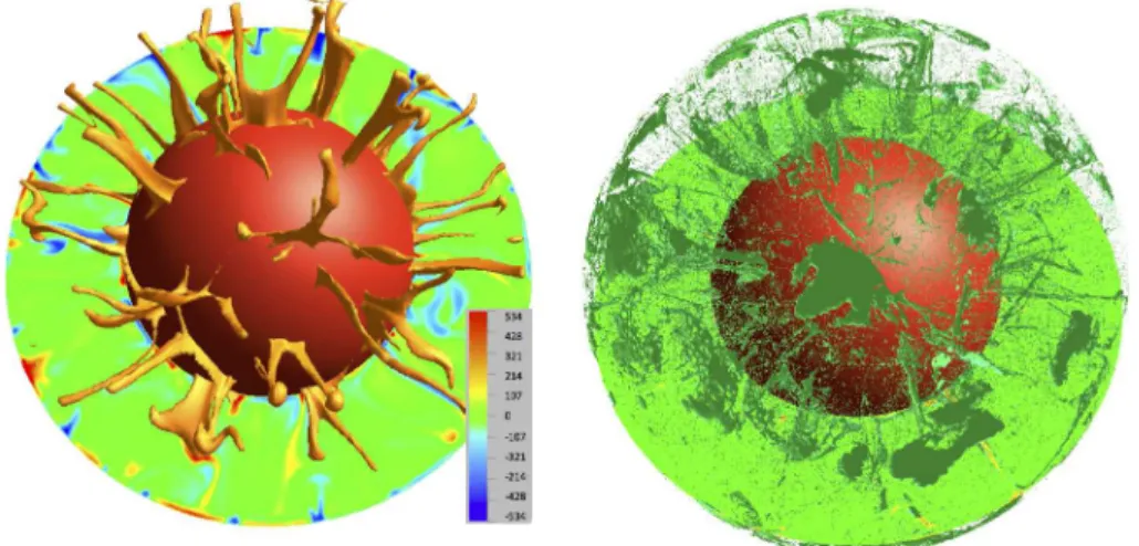
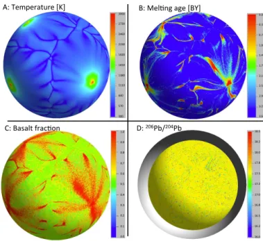
Figure 3 shows snapshots of temperature distribution and bulk composition in the do-15

main. Figure 4 shows snapshots of the temperature, melt production, bulk composition and melting age (i.e. time since melting), at the end of the calculation. The relation-ships between these parameters is clearly visible; in our model, mantle material melts at focussed regions of high temperature close to the surface (plumes), where the bulk composition gets altered. The basalt collects at the surface directly above. From there, 20

(15)

GMDD

8, 9553–9587, 2015

mantle

Title Page

Tables Figures

◭ ◮

Back Close

Full Screen / Esc

Discussion

P

a

per

|

Discussion

P

a

per

|

Discussion

P

a

per

|

Discussion

P

a

per

|

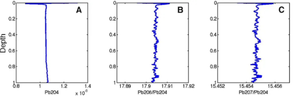
flow (subduction zones). Segregated material has reached the core-mantle boundary (CMB) within 500 million years. (Seen in time series of bulk compositional field and val-ues of the domain rms-velocity which is above 1 cm yr−1; not shown.) The snapshots are representative of the structures as they develop over time; note both the amount of melt produced over time (Fig. 5c), and the increase in the average melting age over 5

time (Fig. 6) are steady. Figure 7 shows the radial distribution of Pb isotopes and Pb isotope ratios radially. The more basaltic rich surface layer shows up as an increase for example in204Pb, while just beneath we see a decrease which goes with the thin underlying residual layer. Deeper in the mantle the figure shows that in this case it is relatively well-mixed with limited variation.

10

3.1 Melting diagnostics

As shown in Fig. 5a our method conserves bulk composition (average value stays constant over time). The figure also shows that the surface average bulk composition becomes more basaltic than the global average, as expected. Figure 5b shows that the total number of particles present in the domain stays roughly constant at a total 15

of 1.2 billion, although particles are continuously merged and split (Fig. 5b). The fact that this method conserves bulk composition shows that the splitting and merging is not affecting the average composition. Figure 5c shows total melt production over time. As shown, there is limited variation in the amount of melt produced as function of time. Melt production never stops.

20

3.2 Pb-pseudo-isochrons vs. melting age distributions

Following Rudge (2006) we can compare our findings with his analytical solution linking pseudo-isochron ages based on Pb-isotope distributions to the distribution of melting ages in the mantle. Using;

235

U

238_U·

(eλ235τddi₋₁₎

(eλ₂₃₈τ_ddi₋₁₎=β, (16)

(16)

GMDD

8, 9553–9587, 2015

mantle

Title Page

Tables Figures

◭ ◮

Back Close

Full Screen / Esc

Discussion

P

a

per

|

Discussion

P

a

per

|

Discussion

P

a

per

|

Discussion

P

a

per

|

where;235U and238U are the abundances of Uranium isotopes;λ235andλ238the decay

constants;τddithe pseudo-isochron ages; andβthe slope of the regression line for the 207

Pb/204Pb vs.206Pb/204Pb-plot.

We can plot the Pb-isotope ratios carried by the particles, for example in the top layer of the model, at different times. Following Rudge (2006) we fit a geometric mean 5

regression line (also known as the reduced major axis regression line, as in Fig. 8) to these data at the different times; i.e. evaluatingβof Eq. (16). Then, using Eq. (16) we can evaluate the pseudo-isochron ageτddi, for each of these different times.

Simi-larly, following Rudge (2006) a pseudo-isochron age can be obtained by looking at the distribution of melting ages in the mantle as follows;

10

(eλ235τddi₋₁₎2

(eλ₂₃₈τ_ddi₋₁₎2 =

E(eλ235Tˆm₋₁₎2

E(eλ₂₃₈_Tˆ

m−1)2

, (17)

where

E f( ˆTm)=

τ_Z_s

0

f(τ)qm(τ)dτ (18)

qm(τ) is the probability density function of the particle melting ages; f(τ) is an

arbi-trary given function e.g. (eλ238Tˆm₋₁₎2_;_τ

ddiis the pseudo-isochron age; ˆTmis a random

15

variable which gives the distributions of the parcel ages that have undergone melting.

τs is the starting age of the model, 3.6 Ga. Rudge’s theory is based on a statistical

box-model and in particular assumes: 1 strong mixing. 2 heavy averaging.

Figure 6 shows the build up ofq_m(τ) over time in our model. Since melt production is fairly constant, the histograms show a steady increase in melting age.

20

Figure 9b shows the time evolution of the obtained pseudo-isochron ages based on Pb isotopes (τddi from Eqs. 16 and 17; black and red curves in Fig. 9b), and particle

(17)

GMDD

8, 9553–9587, 2015

mantle

Title Page

Tables Figures

◭ ◮

Back Close

Full Screen / Esc

Discussion

P

a

per

|

Discussion

P

a

per

|

Discussion

P

a

per

|

Discussion

P

a

per

|

For Fig. 9b; showing Pb isotopes on the surface, our results were subsampled and used only data on Pb isotopes from particles that had undergone melting at least once (had a melting age), and were at the surface layer of the model. For the Pb isotopes sampled at the melt, our results were subsampled and used only data on Pb isotopes from melt that was produced in that time step (i.e. not taking the information from 5

a particle but from the material that moved to the surface due to melting). In this case, the pseudo-isochron has a value of 0 for the first 500 million year of the calculated time since until that time only unfractionated material is sampled.

4 Discussion

We have implemented tracking of radioactively decaying isotope systems in a numeri-10

cal model of mantle convective flows. Through this integration we have a tool that will allow experiments on the evolution of the Earth’s mantle providing stronger constrains on both the spatial and temporal evolution. The key process is fractionation of both bulk composition and trace elements on melting. The algorithm that deals with this process (Sect. 2.6), is built on using particles to track the advection of chemical concentration 15

(bulk composition) and abundances (trace elements) with fluid flow, and move informa-tion between those particles upon melting. An advantage of this method of moving melt (i.e. via information not particles) is that we can consider any degree of melting, not just the quanta of melting that must be considered in algorithms that move particles. This allows us to consider much smaller degrees of melting. This is important for example 20

for incompatible elements in the residue.

By deliberately keeping the system simple we can compare and test the results of our numerical experiments to a quasi-analytical solution (Sect. 3, Rudge, 2006). This solution links the melting time distribution of the whole mantle to the pseudo-isochrons that can be measured in lead isotopes sampled only at the surface of the domain. Fig-25

(18)

GMDD

8, 9553–9587, 2015

mantle

Title Page

Tables Figures

◭ ◮

Back Close

Full Screen / Esc

Discussion

P

a

per

|

Discussion

P

a

per

|

Discussion

P

a

per

|

Discussion

P

a

per

|

the end of the modeled time the misfit is around 2 %. We note that our Eq. (17) from Rudge (2006) assumes (1) a well mixed planet, and (2) that the number of melting events that are averaged before sampling (N) is large (heavy averaging), a general-isation from Rudge et al. (2005). As regards the mixing, we note the homogeneous distribution of Pb isotopes, both radially (Fig. 7), and laterally (Fig. 4d) supports strong 5

mixing. As regards averaging we note that Rudge (2006) suggests that the dependence of the pseudo-isochron age onN is fairly weak. The good match is achieved for both sampling the surface and sampling the melt. When sampling the melt, N=1, while particles sampled at the surface carry the signature of a collection of multiple melt-ing events (largerN). The results presented here also support that the dependence of 10

the pseudo-isochron age on N is weak. The good match gives us confidence in the method and therefore opens the opportunity to extract information about the interior distributions of chemical heterogeneity from surface observations.

The sampling location can be important as can be seen in Fig. 9b, where we show the evolution of the pseudo-isochron based on random sampling across the surface 15

and sampling of the melt just after fractionation. Early on in the calculation, the diff er-ence between our subset sampled at the surface and the melting location is substan-tial mainly because the material sampled at melting locations has not gone through melting and fractionation before, whereas the surface contains fractionated material immediately after the calculation starts. On the long time scale (>BY) the di_fference 20

between the two isochrons is very small, again supporting the idea of a strongly mixed reservoir.

In our model setup, due to the convective pattern resulting from limited variation in viscosity, melting predominantly happens at the top of circular upwellings, i.e. plume like structures. Most melting in the terrestrial mantle (and chemical fractionation) hap-25

(19)

GMDD

8, 9553–9587, 2015

mantle

Title Page

Tables Figures

◭ ◮

Back Close

Full Screen / Esc

Discussion

P

a

per

|

Discussion

P

a

per

|

Discussion

P

a

per

|

Discussion

P

a

per

|

on samples taken at random across the surface vs. those taken at the location of melt production.

Although the pseudo-isochrons we find via the melting ages and lead isotopes are consistent, in absolute value they do deviate from the one observed in lead isotopes in nature. As mentioned already the simulation case presented is intentionally simple 5

to allow a direct comparison with the analytical solution of Rudge (2006), as a result it is not Earth-like in every respect. In particular, the vigour of convection (mean ve-locity 1.5 cm yr−1) is much lower than Earth (current surface velocity 5 cm yr−1 RMS). Also the model vigour is constant, while on Earth it is expected to be more vigorous in the hotter past. The combined effect is that the number of overturns in the simulated 10

case will be many times less than for Earth (Huang and Davies, 2007a). Therefore the number of passages through melting zones will also be much lower in this simulation than Earth. Since this model case is neither Earth-like in its vigour nor its melting a dif-ference between pseudo-isochrons ages is not a surprise. Since more melting would remove more of the older heterogeneities and therefore reduce the pseudo-chron age 15

it might be expected therefore that more realistic models will have the potential to rec-oncile these di_fferences. Future work is planned to investigate this.

Future implementations will be extended with routines to allow trace elements to move to/from both continent and atmosphere reservoirs (for noble gasses), and exten-sions on how chemical structures a_ffect the flow field. The good comparison to analyt-20

ical theory presented in this work, gives confidence that the current implementation is a good basis from which to include more complex and Earth-like processes into future numerical experiments. By doing so we can shift the focus from comparing numerical experiments to analytical solutions, to comparing them to observations.

5 Conclusions

25

(20)

GMDD

8, 9553–9587, 2015

mantle

Title Page

Tables Figures

◭ ◮

Back Close

Full Screen / Esc

Discussion

P

a

per

|

Discussion

P

a

per

|

Discussion

P

a

per

|

Discussion

P

a

per

|

feature of the melting routine is that we transport information between particles, rather than move particles. We showed that our implementation is robust in the sense that (1) it conserves composition, (2) it conserves trace element abundance, (3) it matches the Rudge (2006) quasi-analytical solution for the prediction of isochron ages based on the distribution of melting age and pseudo-isochron ages based on lead isotopes at 5

the surface of the model.

Acknowledgements. We acknowledge the support of NERC NE/H006559/1, NE/K004824/1.

We also acknowledge the support of NERC ARCHER (UK national super computer). The authors acknowledge Andy Heath, Ian Thomas and Ian Merrick for developing the software “MantleVis” used to create Figs. 3 and 4.

10

References

Allègre, C., Brevart, O., Dupré, B., and Minster, J.-F.: Isotopic and chemical effects produced in a continuously differentiating convecting Earth mantle, Philos. T. Roy. Soc. A, 297, 447–477, 1980. 9561

Armstrong, R. L.: A model for the evolution of strontium and lead isotopes in a dynamic earth,

15

Rev. Geophys., 6, 175–199, 1968. 9565

Baumgardner, J. R.: Three-dimensional treatment of convective flow in the Earth’s mantle, J. Stat. Phys., 39, 501–511, 1985. 9557

Baumgardner, J. R. and Frederickson, P. O.: Icosahedral discretization of the two-sphere, SIAM J. Numer. Anal., 22, 1107–1115, 1985. 9557

20

Brandenburg, J. and van Keken, P.: Methods for thermochemical convection in Earth’s mantle with force-balanced plates, Geochem. Geophy. Geosy., 8, Q11004, doi:10.1029/2007GC001692, 2007a. 9556

Brandenburg, J. and Van Keken, P.: Deep storage of oceanic crust in a vigorously convecting mantle, J. Geophys. Res.-Sol. Ea., 112, B06403, doi:10.1029/2006JB004813, 2007b. 9556

25

(21)

GMDD

8, 9553–9587, 2015

mantle

Title Page

Tables Figures

◭ ◮

Back Close

Full Screen / Esc

Discussion

P

a

per

|

Discussion

P

a

per

|

Discussion

P

a

per

|

Discussion

P

a

per

|

Bunge, H.-P. and Baumgardner, J. R.: Mantle convection modeling on parallel virtual machines, Comput. Phys., 9, 207–215, 1995. 9557

Christensen, U. R. and Hofmann, A. W.: Segregation of subducted oceanic crust in the con-vecting mantle, J. Geophys. Res.-Sol. Ea., 99, 19867–19884, 1994. 9555, 9556

Davies, D. R., Davies, J. H., Hassan, O., Morgan, K., and Nithiarasu, P.: Investigations

5

into the applicability of adaptive finite element methods to two-dimensional infinite Prandtl number thermal and thermochemical convection, Geochem. Geophy. Geosy., 8, Q05010, doi:10.1029/2006GC001470, 2007. 9555

Davies, D. R., Davies, J. H., Bollada, P. C., Hassan, O., Morgan, K., and Nithiarasu, P.: A hierarchical mesh refinement technique for global 3-D spherical mantle convection modelling,

10

Geosci. Model Dev., 6, 1095–1107, doi:10.5194/gmd-6-1095-2013, 2013. 9557

Davies, G. F.: Stirring geochemistry in mantle convection models with stiff plates and slabs, Geochim. Cosmochim. Ac., 66, 3125–3142, 2002. 9556

De Smet, J., Van den Berg, A., and Vlaar, N.: Stability and growth of continental shields in mantle convection models including recurrent melt production, Tectonophysics, 296, 15–29,

15

1998. 9556

Huang, J. and Davies, G. F.: Stirring in three-dimensional mantle convection models and implications for geochemistry: passive tracers, Geochem. Geophy. Geosy., 8, Q03017, doi:10.1029/2006GC001312, 2007a. 9556, 9571

Huang, J. and Davies, G. F.: Stirring in three-dimensional mantle convection models and

20

implications for geochemistry: 2. heavy tracers, Geochem. Geophy. Geosy., 8, Q07004, doi:10.1029/2007GC001621, 2007b. 9555, 9556

Huang, J. and Davies, G. F.: Geochemical processing in a three-dimensional regional spherical shell model of mantle convection, Geochem. Geophy. Geosy., 8, Q11006, doi:10.1029/2007GC001625, 2007c. 9556

25

Köstler, C.: Iterative solvers for modeling mantle convection with strongly varying viscosity, PhD thesis, Friedrich-Schiller-Univ. Jena, Germany, 2011. 9557

Lehnert, K., Su, Y., Langmuir, C., Sarbas, B., and Nohl, U.: A global geochemical database structure for rocks, Geochem. Geophy. Geosy., 1, doi:10.1029/1999GC000026, 2000. 9555, 9586

30

(22)

GMDD

8, 9553–9587, 2015

mantle

Title Page

Tables Figures

◭ ◮

Back Close

Full Screen / Esc

Discussion

P

a

per

|

Discussion

P

a

per

|

Discussion

P

a

per

|

Discussion

P

a

per

|

Nakagawa, T., Tackley, P. J., Deschamps, F., and Connolly, J. A.: Incorporating self-consistently calculated mineral physics into thermochemical mantle convection simulations in a 3-D spherical shell and its influence on seismic anomalies in Earth’s mantle, Geochem. Geo-phy. Geosy., 10, Q03004, doi:10.1029/2008GC002280, 2009. 9556

Nakagawa, T., Tackley, P. J., Deschamps, F., and Connolly, J. A.: The influence of MORB and

5

harzburgite composition on thermo-chemical mantle convection in a 3-D spherical shell with self-consistently calculated mineral physics, Earth Planet. Sc. Lett., 296, 403–412, 2010. 9556

Oldham, D. and Davies, J. H.: Numerical investigation of layered convection in a three-dimensional shell with application to planetary mantles, Geochem. Geophy. Geosy., 5,

10

Q12C04, doi:10.1029/2003GC000603, 2004. 9555

Rudge, J. F.: Mantle pseudo-isochrons revisited, Earth Planet. Sc. Lett., 249, 494–513, 2006. 9554, 9556, 9561, 9567, 9568, 9569, 9570, 9571

Rudge, J. F., McKenzie, D., and Haynes, P. H.: A theoretical approach to understanding the iso-topic heterogeneity of mid-ocean ridge basalt, Geochim. Cosmochim. Ac., 69, 3873–3887,

15

2005. 9570

Samuel, H. and Evonuk, M.: Modeling advection in geophysical flows with particle level sets, Geochem. Geophy. Geosy., 11, Q08020, doi:10.1029/2010GC003081, 2010. 9555

Stegman, D. R., Richards, M. A., and Baumgardner, J. R.: Effects of depth-dependent viscos-ity and plate motions on maintaining a relatively uniform mid-ocean ridge basalt reservoir

20

in whole mantle flow, J. Geophys. Res., 107, ETG51–ETG5.8, doi:10.1029/2001JB000192, 2002. 9557

Stegman, D. R., Jellinek, A. M., Zatman, S. A., Baumgardner, J. R., and Richards, M. A.: An early lunar core dynamo driven by thermochemical mantle convection, Nature, 421, 143– 146, 2003. 9557

25

Tackley, P. J.: Mantle geochemical geodynamics, in: Treatise on Geophysics, edited by: Schu-bert, G. and Bercovici, D., Elsevier, Amsterdam, 437–505, 2007. 9555

van Keken, P. E. and Ballentine, C.: Whole-mantle versus layered mantle convection and the role of a high-viscosity lower mantle in terrestrial volatile evolution, Earth Planet. Sc. Lett., 156, 19–32, 1998. 9555

30

(23)

GMDD

8, 9553–9587, 2015

mantle

Title Page

Tables Figures

◭ ◮

Back Close

Full Screen / Esc

Discussion

P

a

per

|

Discussion

P

a

per

|

Discussion

P

a

per

|

Discussion

P

a

per

|

Walzer, U. and Hendel, R.: A new convection-fractionation model for the evolution of the prin-cipal geochemical reservoirs of the Earth’s mantle, Phys. Earth Planet. In., 112, 211–256, 1999. 9556

Xie, S. and Tackley, P. J.: Evolution of U-Pb and Sm-Nd systems in numerical mod-els of mantle convection and plate tectonics, J. Geophys. Res.-Sol. Ea., 109, B11204,

5

doi:10.1029/2004JB003176, 2004a. 9555, 9556

Xie, S. and Tackley, P. J.: Evolution of helium and argon isotopes in a convecting mantle, Phys. Earth Planet. In., 146, 417–439, 2004b. 9556

Yang, W.-S. and Baumgardner, J. R.: A matrix-dependent transfer multigrid method for strongly variable viscosity infinite Prandtl number thermal convection, Geophys. Astro. Fluid, 92, 151–

10

195, 2000. 9557

(24)

GMDD

8, 9553–9587, 2015

mantle

Title Page

Tables Figures

◭ ◮

Back Close

Full Screen / Esc

Discussion

P

a

per

|

Discussion

P

a

per

|

Discussion

P

a

per

|

Discussion

P

a

per

|

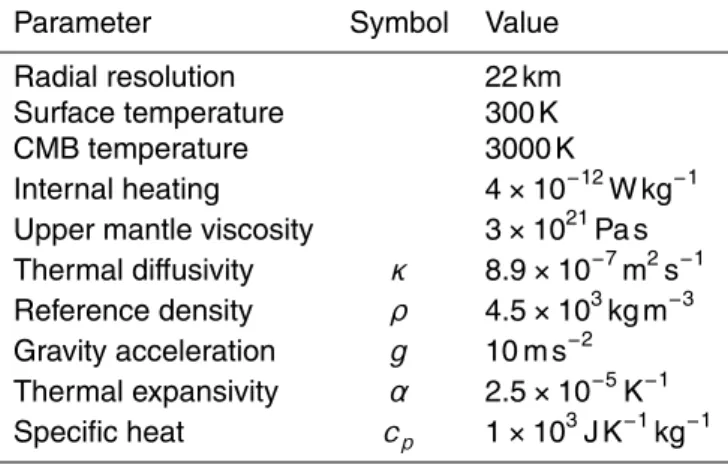
Table 1.Calculation parameters.

Parameter Symbol Value

Radial resolution 22 km Surface temperature 300 K CMB temperature 3000 K

Internal heating 4×10−12W kg−1 Upper mantle viscosity 3_×1021Pa s Thermal di_ffusivity κ 8.9_×10−7m2s−1 Reference density ρ 4.5×103kg m−3 Gravity acceleration g 10 m s−2

(25)

GMDD

8, 9553–9587, 2015

mantle

Title Page

Tables Figures

◭ ◮

Back Close

Full Screen / Esc

Discussion

P

a

per

|

Discussion

P

a

per

|

Discussion

P

a

per

|

Discussion

P

a

per

|

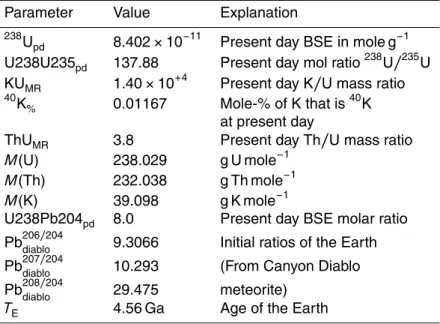
Table 2.Parameters and values used for initialisation of trace elements.

Parameter Value Explanation

238

U_pd 8.402_×10−11 Present day BSE in mole g−1 U238U235_pd 137.88 Present day mol ratio238U/235U KU_MR 1.40×10+4 Present day K/U mass ratio 40

K_% 0.01167 Mole-% of K that is40K at present day

ThU_MR 3.8 Present day Th/U mass ratio M(U) 238.029 g U mole−1

M(Th) 232.038 g Th mole−1 M(K) 39.098 g K mole−1

U238Pb204_pd 8.0 Present day BSE molar ratio

Pb206_diablo/204 9.3066 Initial ratios of the Earth Pb207_diablo/204 10.293 (From Canyon Diablo

(26)

GMDD

8, 9553–9587, 2015

mantle

Title Page

Tables Figures

◭ ◮

Back Close

Full Screen / Esc

Discussion

P

a

per

|

Discussion

P

a

per

|

Discussion

P

a

per

|

Discussion

P

a

per

|

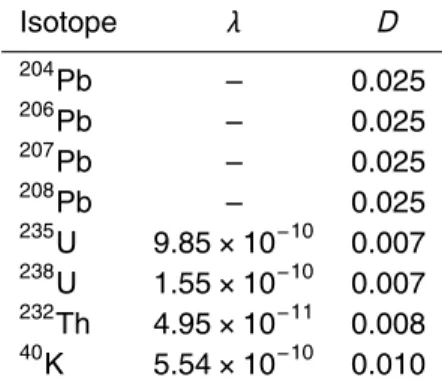
Table 3.Isotope data: Decay constant (λ) in yr−1and partition coefficient (D) of isotopes.

Isotope λ D

204

Pb – 0.025

206

Pb – 0.025

207

Pb – 0.025

208

Pb – 0.025

235

U 9.85×10−10 0.007 238

U 1.55_×10−10 0.007 232

Th 4.95_×10−11 0.008 40

(27)

GMDD

8, 9553–9587, 2015

mantle

Title Page

Tables Figures

◭ ◮

Back Close

Full Screen / Esc

Discussion

P

a

per

|

Discussion

P

a

per

|

Discussion

P

a

per

|

Discussion

P

a

per

|

(28)

GMDD

8, 9553–9587, 2015

mantle

Title Page

Tables Figures

◭ ◮

Back Close

Full Screen / Esc

Discussion

P

a

per

|

Discussion

P

a

per

|

Discussion

P

a

per

|

Discussion

P

a

per

|

Temperature [K]

1000

1500

2000

2500

3000

3500

Depth [km]

0

100

200

300

400

500

600 Solidii for different compositions

Fertile c=0.6 Depleted

(29)

GMDD

8, 9553–9587, 2015

mantle

Title Page

Tables Figures

◭ ◮

Back Close

Full Screen / Esc

Discussion

P

a

per

|

Discussion

P

a

per

|

Discussion

P

a

per

|

Discussion

P

a

per

|

(30)

GMDD

8, 9553–9587, 2015

mantle

Title Page

Tables Figures

◭ ◮

Back Close

Full Screen / Esc

Discussion

P

a

per

|

Discussion

P

a

per

|

Discussion

P

a

per

|

Discussion

P

a

per

|

A:#Temperature#[K]# B:#Mel2ng#age#[BY]#

C:#Basalt#frac2on# D:#206_Pb/204_Pb#

0.0 0.3 0.7 1.0 1.4# 1.7# 2.1# 2.5# 2.9 3.2# 3.6#

18.5# 18.2# 18.0# 17.8# 17.5# 17.2# 17.0# 16.8# 16.5# 16.2# 16.0# 1.0#

0.9# 0.8# 0.7# 0.6# 0.5# 0.4# 0.3# 0.2# 0.1# 0.0# 3000# 2730# 2460# 2190# 1920# 1650# 1380# 1110# 840# 570# 300#

(31)

GMDD

8, 9553–9587, 2015

mantle

Title Page

Tables Figures

◭ ◮

Back Close

Full Screen / Esc

Discussion

P

a

per

|

Discussion

P

a

per

|

Discussion

P

a

per

|

Discussion

P

a

per

|

(32)

GMDD

8, 9553–9587, 2015

mantle

Title Page

Tables Figures

◭ ◮

Back Close

Full Screen / Esc

Discussion

P

a

per

|

Discussion

P

a

per

|

Discussion

P

a

per

|

Discussion

P

a

per

|

(33)

GMDD

8, 9553–9587, 2015

mantle

Title Page

Tables Figures

◭ ◮

Back Close

Full Screen / Esc

Discussion

P

a

per

|

Discussion

P

a

per

|

Discussion

P

a

per

|

Discussion

P

a

per

|

(34)

GMDD

8, 9553–9587, 2015

mantle

Title Page

Tables Figures

◭ ◮

Back Close

Full Screen / Esc

Discussion

P

a

per

|

Discussion

P

a

per

|

Discussion

P

a

per

|

Discussion

P

a

per

|

206

Pb /

204

Pb

17

18

19

20

207

Pb /

204

Pb

15.3

15.35

15.4

15.45

15.5

15.55

15.6

15.65

15.7

pseudo-isochron age = 1.85 Ga

Natural data; Lead isotopes for basalt

Samples

Regression line

(35)

GMDD

8, 9553–9587, 2015

mantle

Title Page

Tables Figures

◭ ◮

Back Close

Full Screen / Esc

Discussion

P

a

per

|

Discussion

P

a

per

|

Discussion

P

a

per

|

Discussion

P

a

per

|